
DALib: A Curated Repository of Libraries for Data Augmentation in Computer Vision


Abstract
:1. Introduction
- Computer Vision—Data augmentation is extensively employed in computer vision tasks, such as image classification, object detection, and semantic segmentation. By applying transformations like rotations, translations, flips, zooms, and color variations, data augmentation helps models learn to recognize objects from different perspectives, lighting conditions, scales, and orientations [1,2,3,4]. This enhances the generalization ability of the models and makes them more robust to variations in real-world images.
- Natural Language Processing (NLP)—Data augmentation techniques are also applicable to NLP tasks, including text classification, sentiment analysis, and machine translation [5,6,7]. Methods like back-translation, word replacement, and synonym substitution can be used to generate augmented text samples, effectively increasing the diversity of the training data and improving the language model’s understanding and generalization.
- Speech Recognition—In speech recognition tasks, data augmentation techniques can be used to introduce variations in audio samples, such as adding background noise, altering pitch or speed, or applying reverberations [8,9,10]. Augmenting the training data with these transformations helps a model to be more robust to different acoustic environments and improves its performance in real-world scenarios.
- Time Series Analysis—Data augmentation can be applied to time series data, such as sensor data, stock market data, or physiological signals. Techniques like time warping, scaling, jittering, and random noise injection can create augmented samples that capture various temporal patterns, trends, and noise characteristics [11,12,13]. Augmentation in time series data helps models to learn and generalize better to different temporal variations and noisy conditions.
- Medical Imaging—In the field of medical imaging, data augmentation is crucial due to the scarcity and high cost of labeled data. Augmentation techniques such as rotations, translations, and elastic deformations can simulate anatomical variations, different imaging angles, and distortions in medical images [14,15,16,17]. By augmenting the dataset, models trained on limited labeled medical images can generalize better and be more robust to variability in patient anatomy and imaging conditions.
- Anomaly Detection—Data augmentation can be used to create artificial anomalies or perturbations in normal data samples, thereby generating augmented data that contains both normal and anomalous instances [18,19,20]. This augmented dataset can then be used for training anomaly detection models, enabling them to learn a wider range of normal and abnormal patterns and improving their detection accuracy.
- We collect information on data augmentation libraries designed for computer vision applications. Existing reviews focus on data augmentation methods and not on the availability of such methods in public libraries;
- Our work is not limited to a specific application scenario. The libraries have been chosen to offer the readers a comprehensive survey of available methods to be used in different computer vision applications;
- To the best of our knowledge, this is the first comprehensive review of data augmentation libraries that also offers a curated taxonomy;
- We also provide a dedicated public website to serve as a centralized repository where the taxonomy, methods, and examples associated with the surveyed data augmentation can be explored;
- This is an ongoing work that will be expanded when new libraries become available.
2. Data Augmentation Libraries
2.1. Albumentations
2.2. AugLy
2.3. Augmentor
2.4. Augraphy
2.5. Automold
2.6. CLoDSA
2.7. imgaug
2.8. KerasCV
2.9. Kornia
2.10. SOLT
2.11. Torchvision
3. Data Augmentation Taxonomy
4. Data Augmentation Techniques
4.1. Generic Traditional Techniques
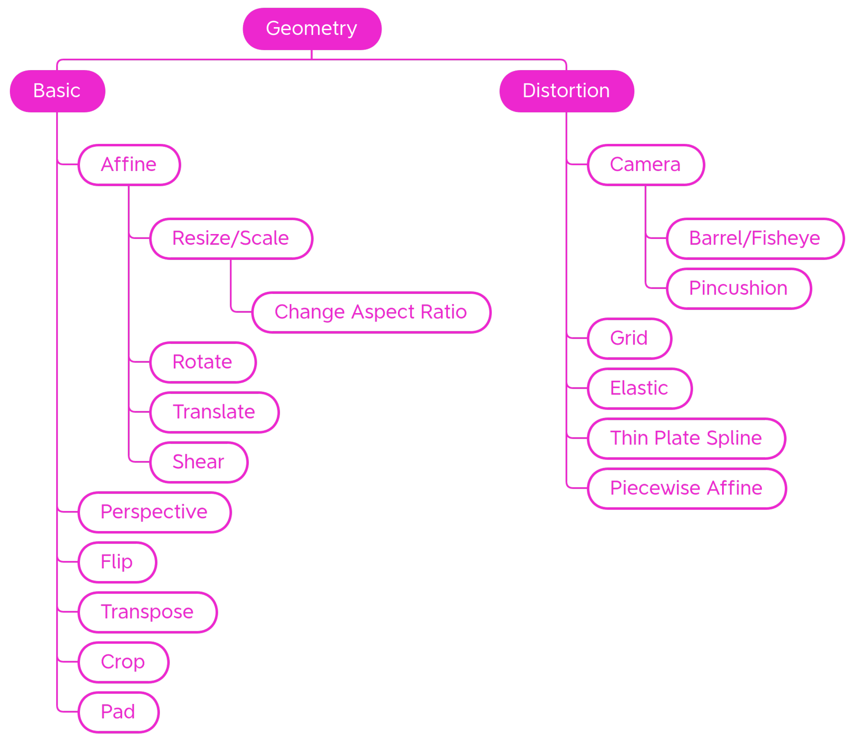
4.1.1. Geometry
Basic
Distortion
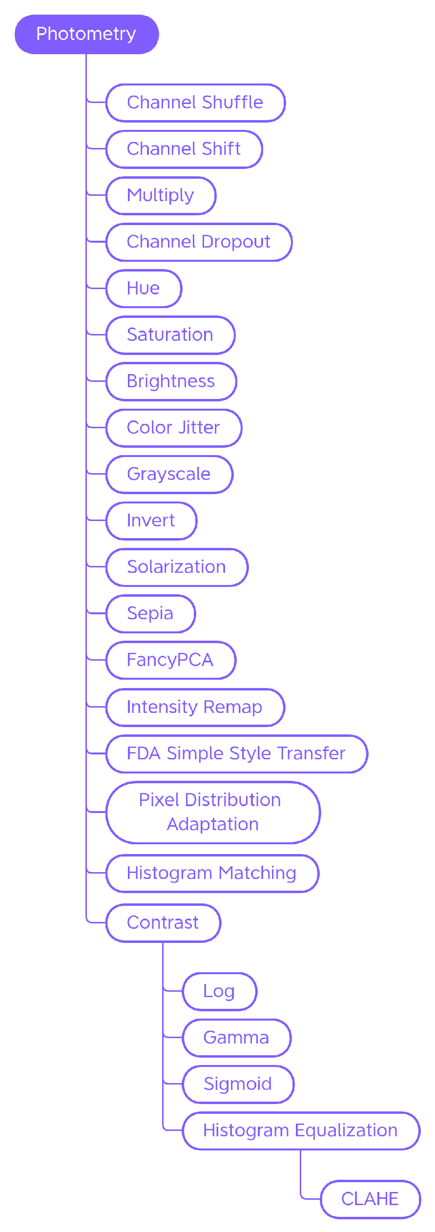
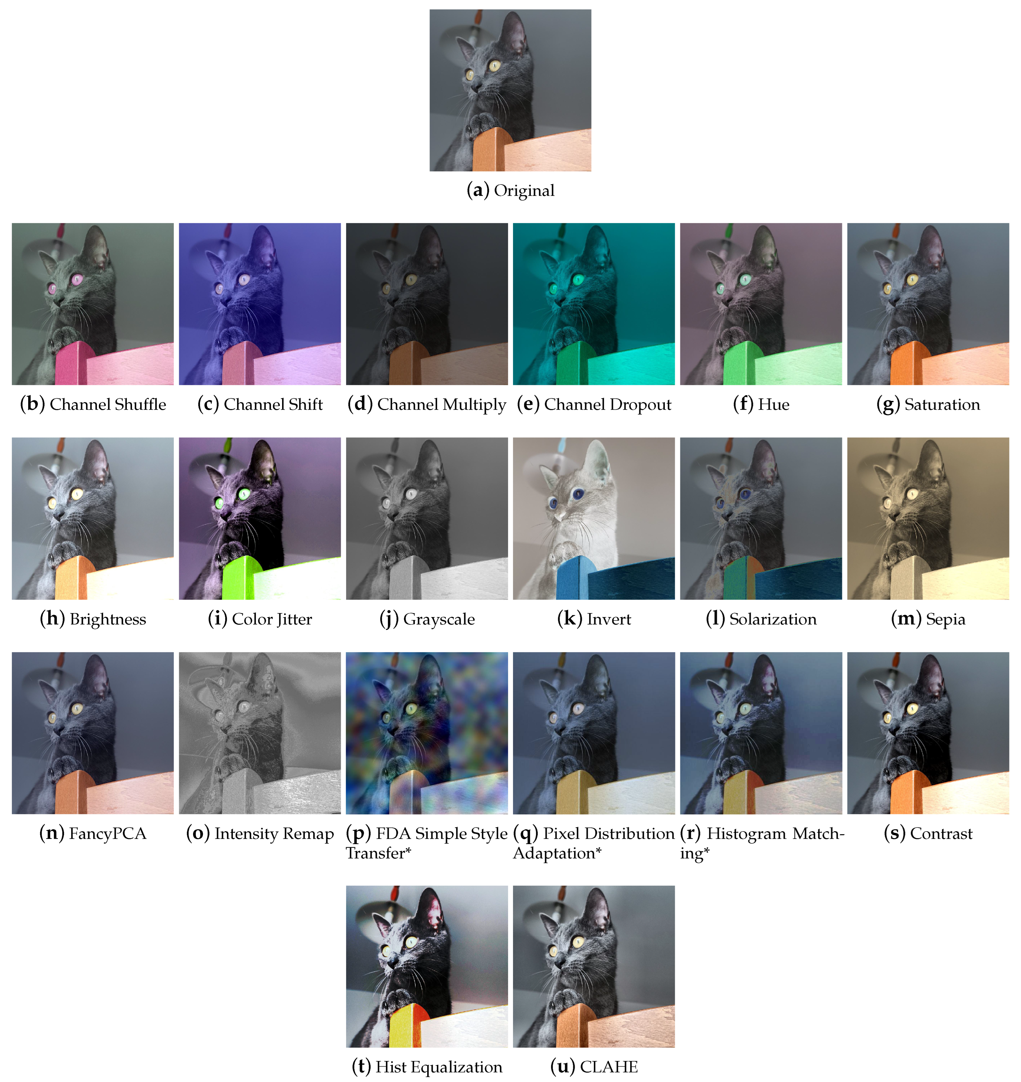
4.1.2. Photometry
Contrast
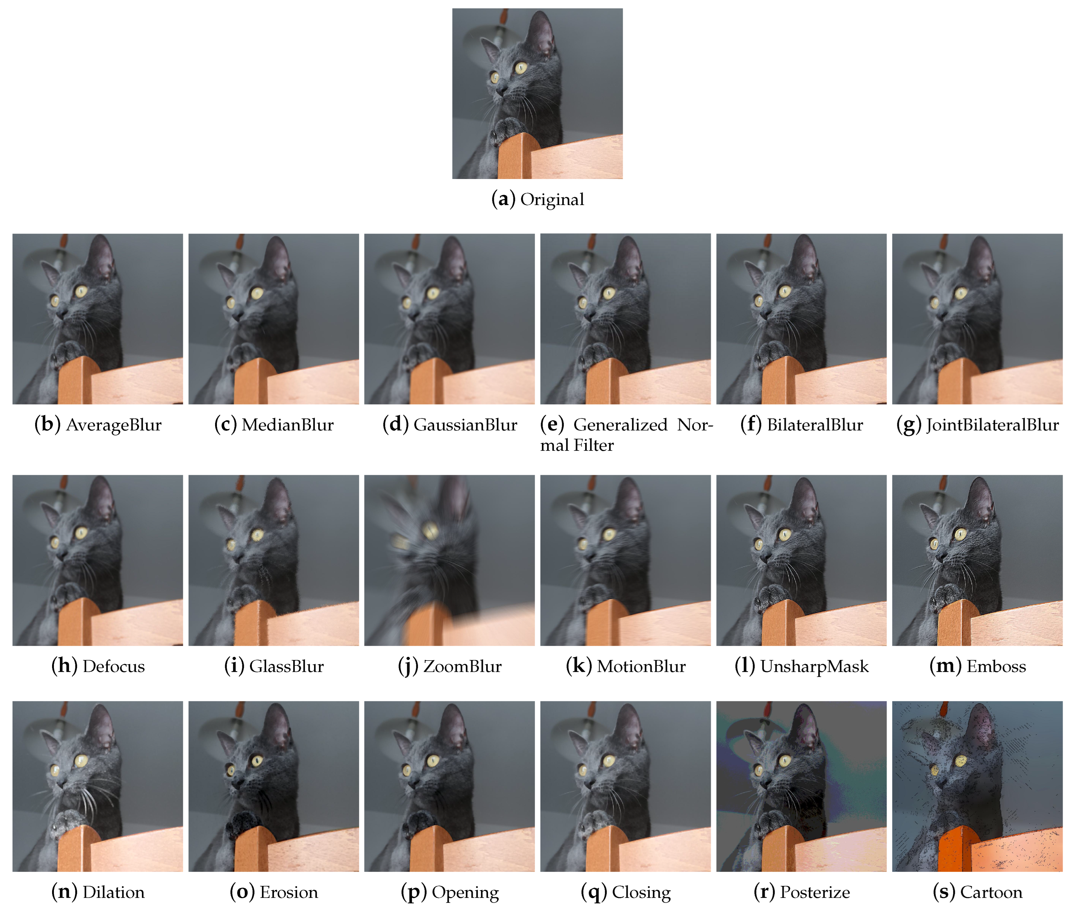
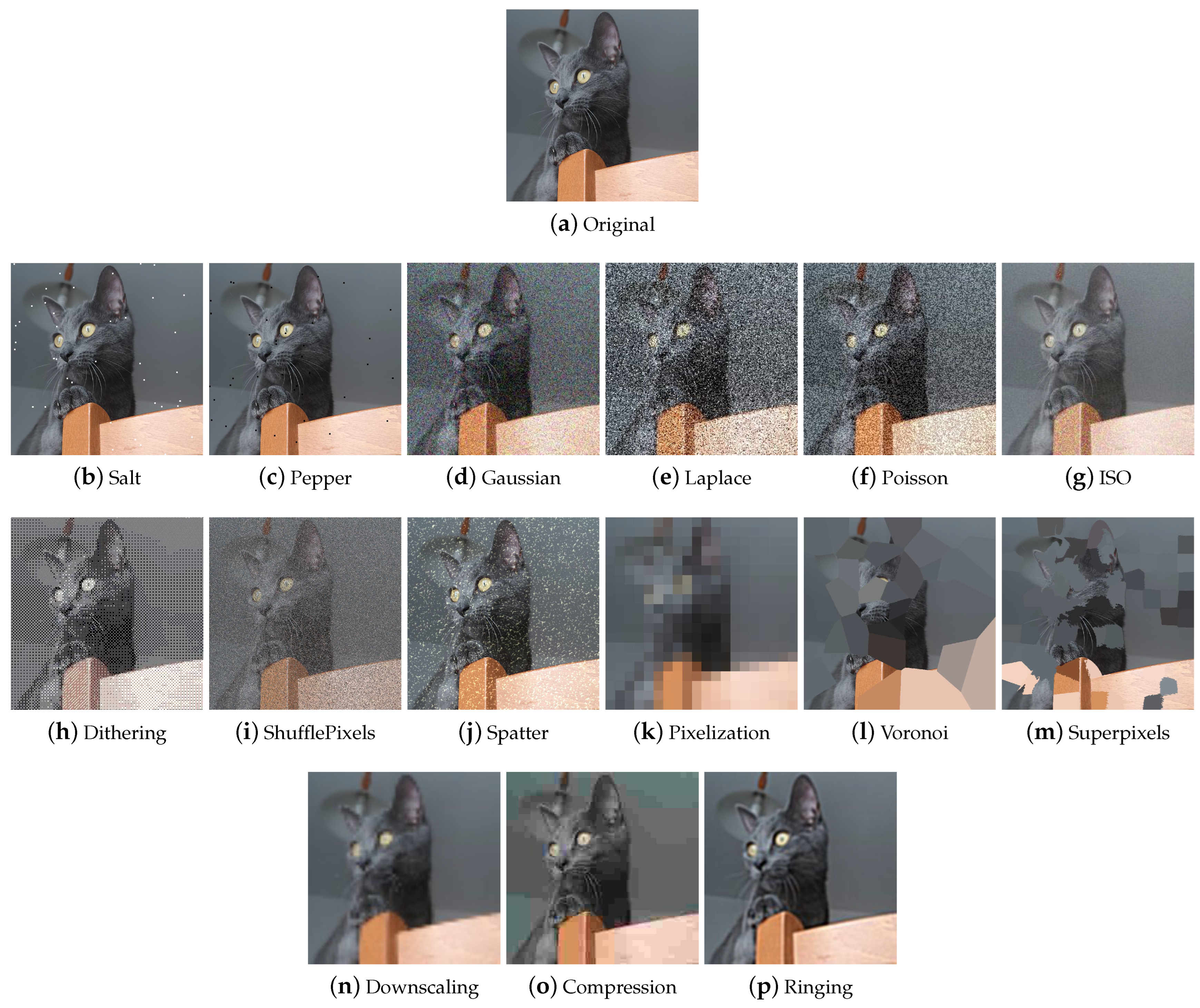
4.1.3. Quality
Blur Filters
Sharpening Techniques
Mathematical Morphology
Style Filters
Noise Injection
Tessellation
Other Worsening Techniques
4.1.4. Miscellaneous
Regional Dropout
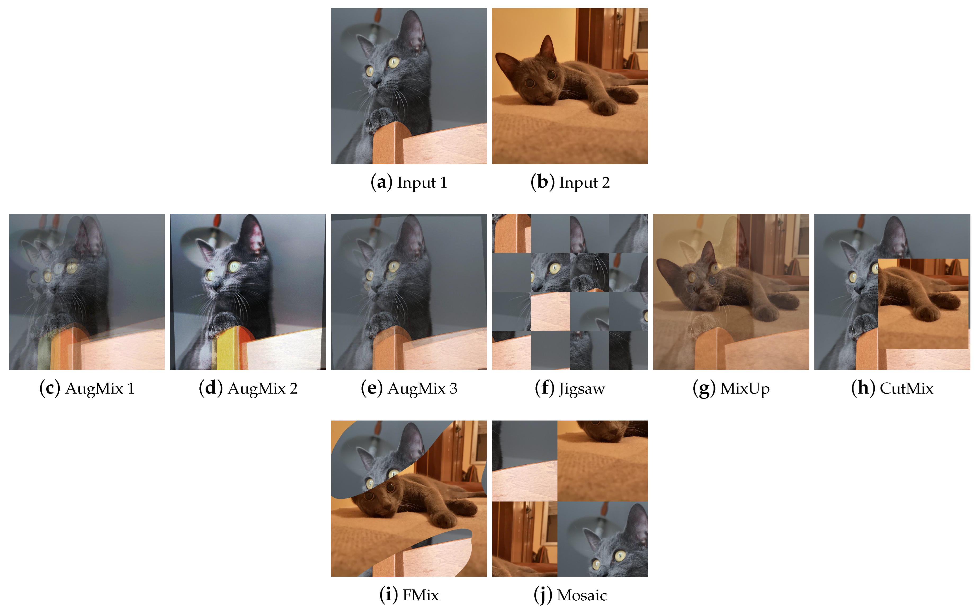
Composition
4.2. Task-Driven Traditional Techniques
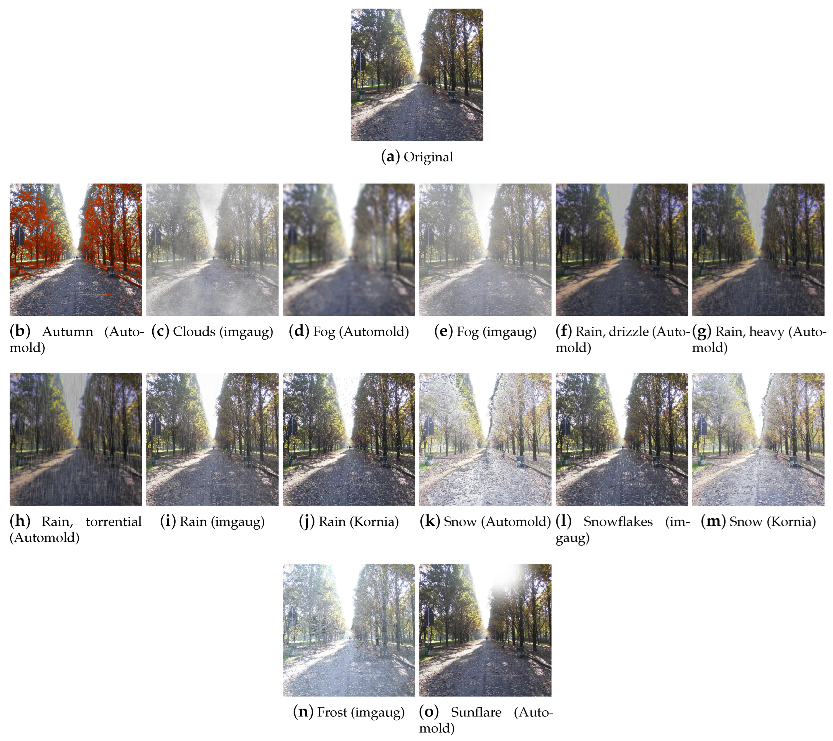
4.2.1. Weather
4.2.2. Street
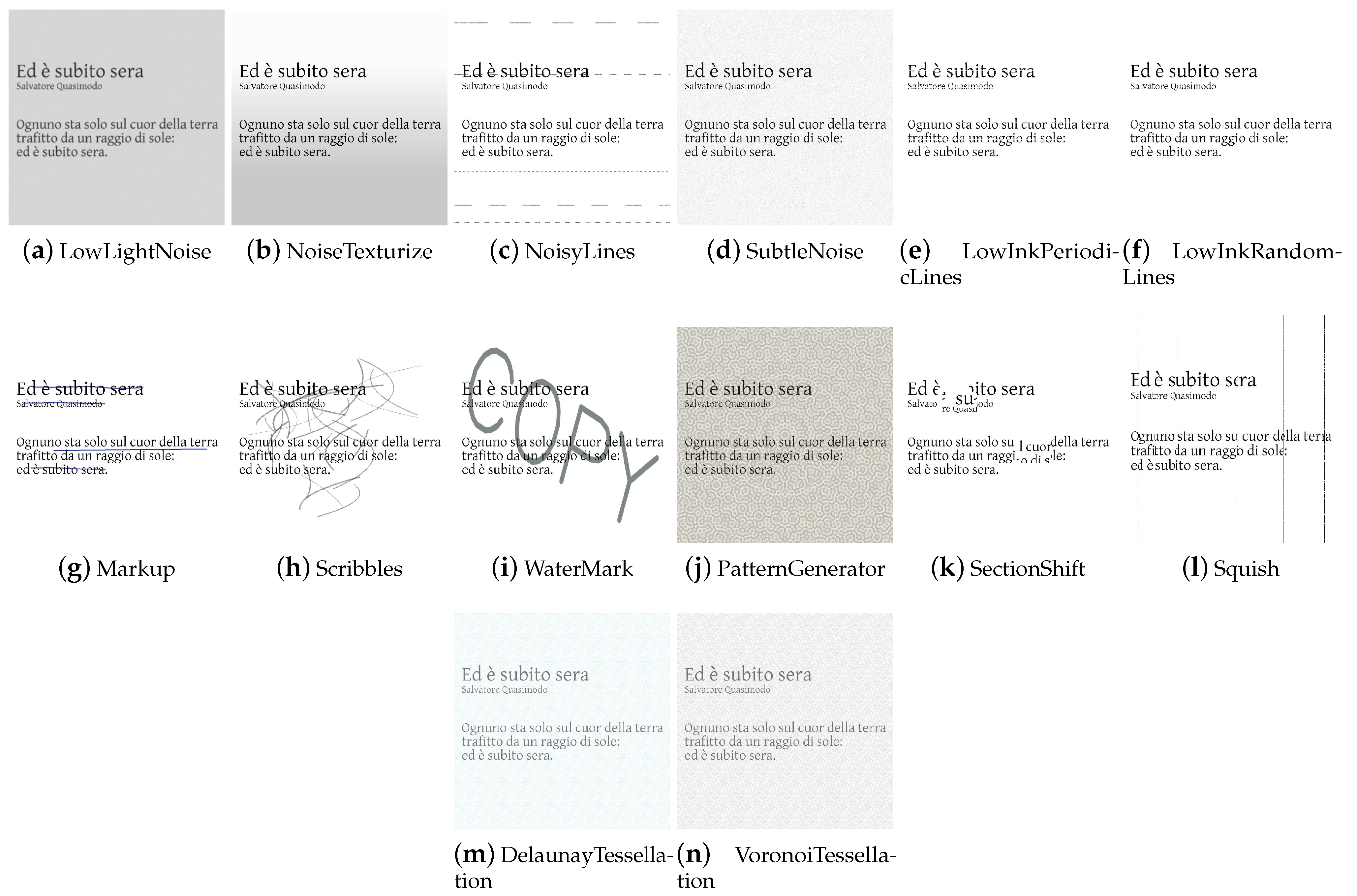
4.2.3. Paper Documents
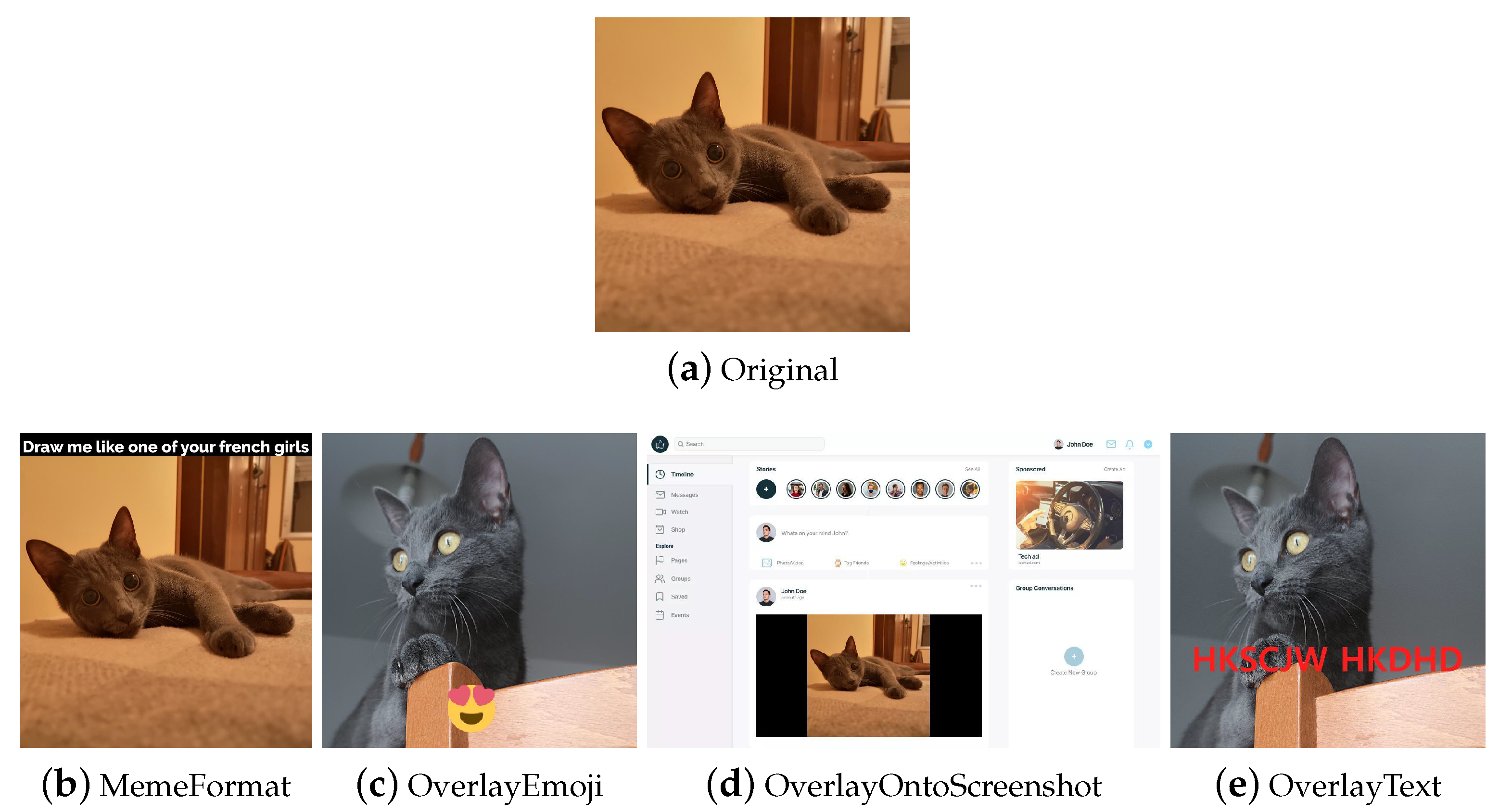
4.2.4. Social Network
4.3. Generative Deep Learning
4.3.1. GANs
4.3.2. VAE
4.3.3. Diffusion Models
4.3.4. Style Transfer
5. The DALib Website
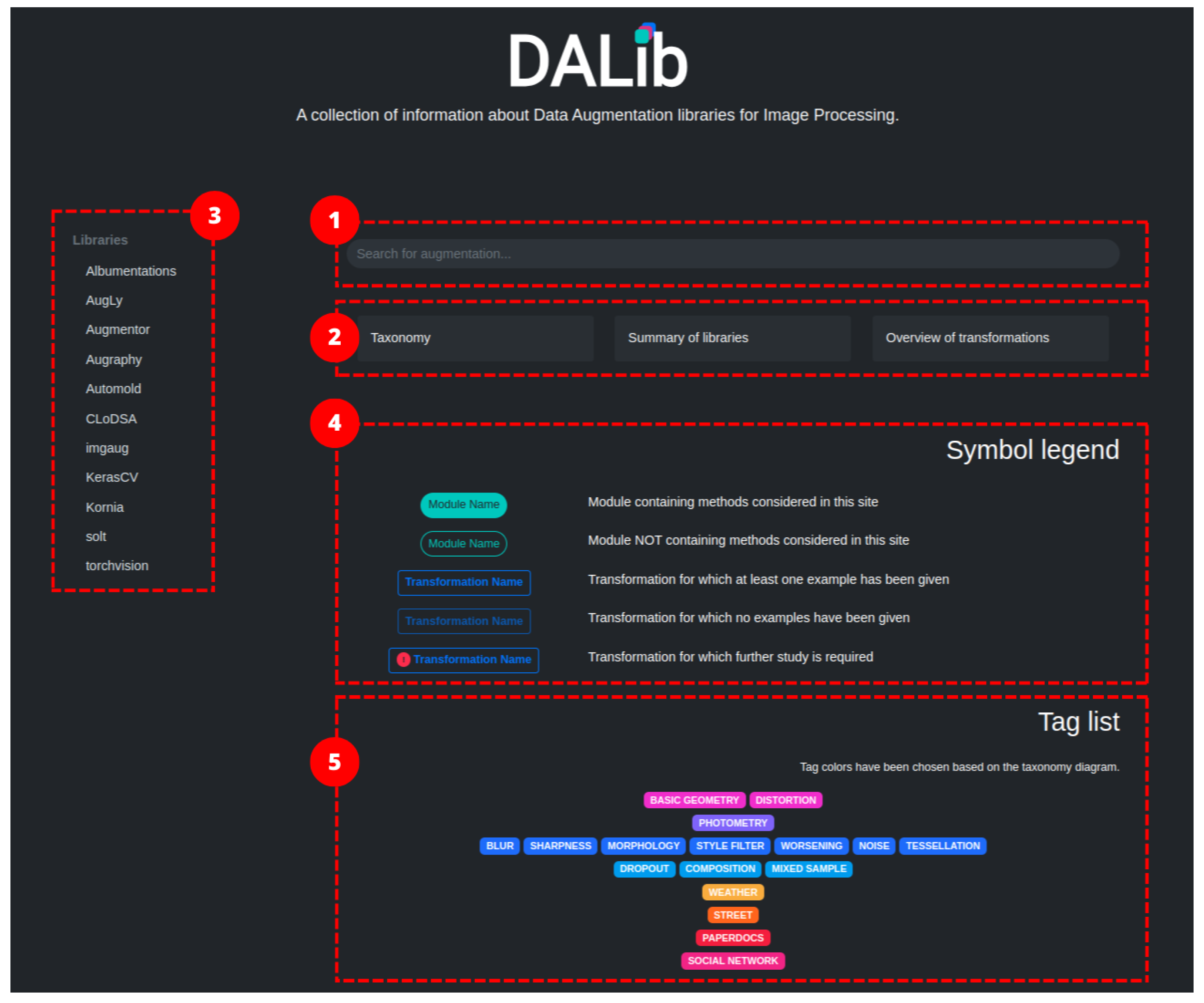
5.1. The Homepage
5.2. The Taxonomy Page
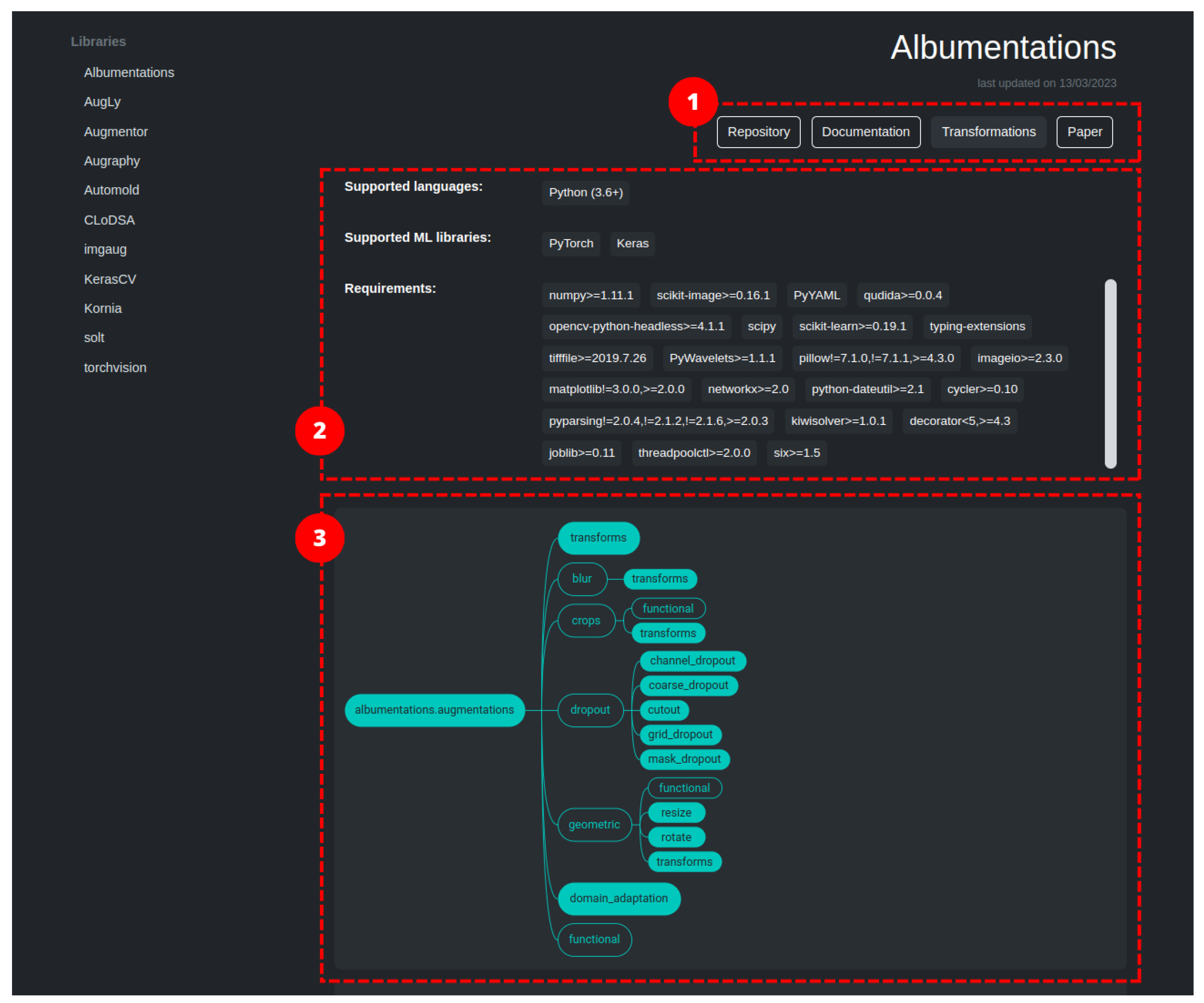
5.3. The Library Pages
5.4. A Few Use Cases
6. Challenges
7. Conclusions
Author Contributions
Funding
Institutional Review Board Statement
Informed Consent Statement
Data Availability Statement
Conflicts of Interest
References
- Zoph, B.; Cubuk, E.D.; Ghiasi, G.; Lin, T.Y.; Shlens, J.; Le, Q.V. Learning data augmentation strategies for object detection. In Proceedings of the Computer Vision–ECCV 2020: 16th European Conference, Glasgow, UK, 23–28 August 2020; Proceedings, Part XXVII 16. Springer: Berlin/Heidelberg, Germany, 2020; pp. 566–583. [Google Scholar]
- Nanni, L.; Paci, M.; Brahnam, S.; Lumini, A. Comparison of different image data augmentation approaches. J. Imaging 2021, 7, 254. [Google Scholar] [CrossRef] [PubMed]
- Khalifa, N.E.; Loey, M.; Mirjalili, S. A comprehensive survey of recent trends in deep learning for digital images augmentation. Artif. Intell. Rev. 2022, 55, 2351–2377. [Google Scholar] [CrossRef]
- Alomar, K.; Aysel, H.I.; Cai, X. Data Augmentation in Classification and Segmentation: A Survey and New Strategies. J. Imaging 2023, 9, 46. [Google Scholar] [CrossRef]
- Feng, S.Y.; Gangal, V.; Wei, J.; Chandar, S.; Vosoughi, S.; Mitamura, T.; Hovy, E. A survey of data augmentation approaches for NLP. arXiv 2021, arXiv:2105.03075. [Google Scholar]
- Shorten, C.; Khoshgoftaar, T.M.; Furht, B. Text data augmentation for deep learning. J. Big Data 2021, 8, 101. [Google Scholar] [CrossRef]
- Li, B.; Hou, Y.; Che, W. Data augmentation approaches in natural language processing: A survey. AI Open 2022, 3, 71–90. [Google Scholar] [CrossRef]
- Ko, T.; Peddinti, V.; Povey, D.; Seltzer, M.L.; Khudanpur, S. A study on data augmentation of reverberant speech for robust speech recognition. In Proceedings of the 2017 IEEE International Conference on Acoustics, Speech and Signal Processing (ICASSP), New Orleans, LA, USA, 5–9 March 2017; pp. 5220–5224. [Google Scholar]
- Park, D.S.; Chan, W.; Zhang, Y.; Chiu, C.C.; Zoph, B.; Cubuk, E.D.; Le, Q.V. SpecAugment: A simple data augmentation method for automatic speech recognition. arXiv 2019, arXiv:1904.08779. [Google Scholar]
- Meng, L.; Xu, J.; Tan, X.; Wang, J.; Qin, T.; Xu, B. Mixspeech: Data augmentation for low-resource automatic speech recognition. In Proceedings of the ICASSP 2021—2021 IEEE International Conference on Acoustics, Speech and Signal Processing (ICASSP), Toronto, ON, Canada, 6–11 June 2021; pp. 7008–7012. [Google Scholar]
- Le Guennec, A.; Malinowski, S.; Tavenard, R. Data augmentation for time series classification using convolutional neural networks. In Proceedings of the ECML/PKDD Workshop on Advanced Analytics and Learning on Temporal Data, Riva del Garda, Italy, 19–23 September 2016. [Google Scholar]
- Wen, Q.; Sun, L.; Yang, F.; Song, X.; Gao, J.; Wang, X.; Xu, H. Time series data augmentation for deep learning: A survey. arXiv 2020, arXiv:2002.12478. [Google Scholar]
- Bandara, K.; Hewamalage, H.; Liu, Y.H.; Kang, Y.; Bergmeir, C. Improving the accuracy of global forecasting models using time series data augmentation. Pattern Recognit. 2021, 120, 108148. [Google Scholar] [CrossRef]
- Shin, H.C.; Tenenholtz, N.A.; Rogers, J.K.; Schwarz, C.G.; Senjem, M.L.; Gunter, J.L.; Andriole, K.P.; Michalski, M. Medical image synthesis for data augmentation and anonymization using generative adversarial networks. In Proceedings of the Simulation and Synthesis in Medical Imaging: Third International Workshop, SASHIMI 2018, Held in Conjunction with MICCAI 2018, Granada, Spain, 16 September 2018; Proceedings 3. Springer: Berlin/Heidelberg, Germany, 2018; pp. 1–11. [Google Scholar]
- Chlap, P.; Min, H.; Vandenberg, N.; Dowling, J.; Holloway, L.; Haworth, A. A review of medical image data augmentation techniques for deep learning applications. J. Med. Imaging Radiat. Oncol. 2021, 65, 545–563. [Google Scholar] [CrossRef]
- Garcea, F.; Serra, A.; Lamberti, F.; Morra, L. Data augmentation for medical imaging: A systematic literature review. Comput. Biol. Med. 2022, 152, 106391. [Google Scholar] [CrossRef]
- Kebaili, A.; Lapuyade-Lahorgue, J.; Ruan, S. Deep Learning Approaches for Data Augmentation in Medical Imaging: A Review. J. Imaging 2023, 9, 81. [Google Scholar] [CrossRef] [PubMed]
- Lim, S.K.; Loo, Y.; Tran, N.T.; Cheung, N.M.; Roig, G.; Elovici, Y. Doping: Generative data augmentation for unsupervised anomaly detection with gan. In Proceedings of the 2018 IEEE International Conference on Data Mining (ICDM), Singapore, 17–20 November 2018; pp. 1122–1127. [Google Scholar]
- Lu, H.; Du, M.; Qian, K.; He, X.; Wang, K. GAN-based data augmentation strategy for sensor anomaly detection in industrial robots. IEEE Sens. J. 2021, 22, 17464–17474. [Google Scholar] [CrossRef]
- Li, Y.; Shi, Z.; Liu, C.; Tian, W.; Kong, Z.; Williams, C.B. Augmented time regularized generative adversarial network (atr-gan) for data augmentation in online process anomaly detection. IEEE Trans. Autom. Sci. Eng. 2021, 19, 3338–3355. [Google Scholar] [CrossRef]
- Buslaev, A.; Iglovikov, V.I.; Khvedchenya, E.; Parinov, A.; Druzhinin, M.; Kalinin, A.A. Albumentations: Fast and Flexible Image Augmentations. Information 2020, 11, 125. [Google Scholar] [CrossRef]
- Papakipos, Z.; Bitton, J. AugLy: Data Augmentations for Robustness. arXiv 2022, arXiv:2201.06494. [Google Scholar]
- Bloice, M.D.; Stocker, C.; Holzinger, A. Augmentor: An Image Augmentation Library for Machine Learning. arXiv 2017, arXiv:1708.04680. [Google Scholar] [CrossRef]
- Groleau, A.; Chee, K.W.; Larson, S.; Maini, S.; Boarman, J. Augraphy: A Data Augmentation Library for Document Images. arXiv 2023, arXiv:2208.14558. [Google Scholar]
- Ujjwal Saxena. Automold—Road Augmentation Library. 2018. Available online: https://github.com/UjjwalSaxena/Automold--Road-Augmentation-Library (accessed on 10 October 2023).
- Casado-García, Á.; Domínguez, C.; García-Domínguez, M.; Heras, J.; Inés, A.; Mata, E.; Pascual, V. CLoDSA: A tool for augmentation in classification, localization, detection, semantic segmentation and instance segmentation tasks. BMC Bioinform. 2019, 20, 323. [Google Scholar] [CrossRef]
- Jung, A.B.; Wada, K.; Crall, J.; Tanaka, S.; Graving, J.; Reinders, C.; Yadav, S.; Banerjee, J.; Vecsei, G.; Kraft, A.; et al. Imgaug. 2020. Available online: https://github.com/aleju/imgaug (accessed on 1 February 2020).
- KerasCV. 2022. Available online: https://github.com/keras-team/keras-cv (accessed on 10 October 2023).
- Riba, E.; Mishkin, D.; Ponsa, D.; Rublee, E.; Bradski, G. Kornia: An open source differentiable computer vision library for pytorch. In Proceedings of the IEEE/CVF Winter Conference on Applications of Computer Vision, Snowmass, CO, USA, 1–5 March 2020; pp. 3674–3683. [Google Scholar]
- Tiulpin, A. SOLT: Streaming over Lightweight Transformations. 2019. Available online: https://zenodo.org/records/3702819 (accessed on 10 October 2023).
- TorchVision Maintainers and Contributors. TorchVision: PyTorch’s Computer Vision Library. 2016. Available online: https://github.com/pytorch/vision (accessed on 10 October 2023).
- Bradski, G. The OpenCV Library. Dr. Dobb’S J. Softw. Tools 2000, 25, 120–123. [Google Scholar]
- Rombach, R.; Blattmann, A.; Lorenz, D.; Esser, P.; Ommer, B. High-resolution image synthesis with latent diffusion models. In Proceedings of the IEEE/CVF Conference on Computer Vision and Pattern Recognition, New Orleans, LA, USA, 18–24 June 2022; pp. 10684–10695. [Google Scholar]
- Cubuk, E.D.; Zoph, B.; Mané, D.; Vasudevan, V.; Le, Q.V. AutoAugment: Learning Augmentation Strategies From Data. In Proceedings of the 2019 IEEE/CVF Conference on Computer Vision and Pattern Recognition (CVPR), Long Beach, CA, USA, 15–20 June 2019; pp. 113–123. [Google Scholar]
- Gonzalez, R.C.; Woods, R.E. Digital Image Processing, 4th ed.; Global Edition; Springer: Berlin/Heidelberg, Germany, 2018. [Google Scholar]
- Hartley, R.; Zisserman, A. Multiple View Geometry in Computer Vision; Cambridge University Press: Cambridge, UK, 2003. [Google Scholar]
- Bookstein, F.L. Principal warps: Thin-plate splines and the decomposition of deformations. IEEE Trans. Pattern Anal. Mach. Intell. 1989, 11, 567–585. [Google Scholar] [CrossRef]
- Simard, P.; Steinkraus, D.; Platt, J. Best practices for convolutional neural networks applied to visual document analysis. In Proceedings of the Seventh International Conference on Document Analysis and Recognition, Edinburgh, UK, 6 August 2003; pp. 958–963. [Google Scholar] [CrossRef]
- Hecht, E. Optics; Pearson Education India: Noida, India, 2012. [Google Scholar]
- BT Series. Studio Encoding Parameters of Digital Television for Standard 4: 3 and Wide-Screen 16: 9 Aspect Ratios; International Telecommunication Union, Radiocommunication Sector: Geneva, Switzerland, 2011. [Google Scholar]
- Poynton, C.A. Rehabilitation of gamma. In Proceedings of the Human Vision and Electronic Imaging III, San Jose, CA, USA, 24–30 January 1998; Rogowitz, B.E., Pappas, T.N., Eds.; International Society for Optics and Photonics, SPIE: Bellingham, WA, USA, 1998; Volume 3299, pp. 232–249. [Google Scholar] [CrossRef]
- Stokes, M.; Anderson, M.; Chandrasekar, S.; Motta, R. A Standard Default Color Space for the Internet-Srgb. 1996. Available online: http://www.w3.org/Graphics/Color/sRGB.html (accessed on 10 October 2023).
- Toub, S. Sepia Tone, StringLogicalComparer, and More. 2005. Available online: https://learn.microsoft.com/en-us/archive/msdn-magazine/2005/january/net-matters-sepia-tone-stringlogicalcomparer-and-more (accessed on 10 October 2023).
- Russ, J. The Image Processing Handbook; CRC Press: Boca Raton, FL, USA, 2002. [Google Scholar]
- Hesse, L.S.; Kuling, G.; Veta, M.; Martel, A.L. Intensity augmentation for domain transfer of whole breast segmentation in MRI. arXiv 2019, arXiv:1909.02642. [Google Scholar]
- Zini, S.; Gomez-Villa, A.; Buzzelli, M.; Twardowski, B.; Bagdanov, A.D.; van de Weijer, J. Planckian Jitter: Countering the color-crippling effects of color jitter on self-supervised training. arXiv 2022, arXiv:2202.07993. [Google Scholar]
- Krizhevsky, A.; Sutskever, I.; Hinton, G.E. ImageNet Classification with Deep Convolutional Neural Networks. In Advances in Neural Information Processing Systems; Pereira, F., Burges, C., Bottou, L., Weinberger, K., Eds.; Curran Associates, Inc.: New York City, NY, USA, 2012; Volume 25. [Google Scholar]
- Achanta, R.; Shaji, A.; Smith, K.; Lucchi, A.; Fua, P.; Süsstrunk, S. SLIC superpixels compared to state-of-the-art superpixel methods. IEEE Trans. Pattern Anal. Mach. Intell. 2012, 34, 2274–2282. [Google Scholar] [CrossRef]
- Moller, J. Lectures on Random Voronoi Tessellations; Springer Science & Business Media: Berlin/Heidelberg, Germany, 2012; Volume 87. [Google Scholar]
- Wang, X.; Xie, L.; Dong, C.; Shan, Y. Real-esrgan: Training real-world blind super-resolution with pure synthetic data. In Proceedings of the IEEE/CVF International Conference on Computer Vision, Montreal, BC, Canada, 11–17 October 2021; pp. 1905–1914. [Google Scholar]
- Zhong, Z.; Zheng, L.; Kang, G.; Li, S.; Yang, Y. Random erasing data augmentation. In Proceedings of the AAAI Conference on Artificial Intelligence, New York, NY, USA, 7–12 February 2020; Volume 34, pp. 13001–13008. [Google Scholar]
- Chen, P.; Liu, S.; Zhao, H.; Jia, J. GridMask Data Augmentation. arXiv 2020, arXiv:2001.04086. [Google Scholar]
- DeVries, T.; Taylor, G.W. Improved Regularization of Convolutional Neural Networks with Cutout. arXiv 2017, arXiv:1708.04552. [Google Scholar]
- Guo, R. Severstal: Steel Defect Detection. 2019. Available online: https://www.kaggle.com/c/severstal-steel-defect-detection/discussion/114254 (accessed on 10 October 2023).
- Hendrycks, D.; Mu, N.; Cubuk, E.D.; Zoph, B.; Gilmer, J.; Lakshminarayanan, B. AugMix: A Simple Data Processing Method to Improve Robustness and Uncertainty. arXiv 2019, arXiv:1912.02781. [Google Scholar]
- Zhang, H.; Cisse, M.; Dauphin, Y.N.; Lopez-Paz, D. mixup: Beyond empirical risk minimization. arXiv 2017, arXiv:1710.09412. [Google Scholar]
- Zhang, Z.; He, T.; Zhang, H.; Zhang, Z.; Xie, J.; Li, M. Bag of freebies for training object detection neural networks. arXiv 2019, arXiv:1902.04103. [Google Scholar]
- Yun, S.; Han, D.; Oh, S.J.; Chun, S.; Choe, J.; Yoo, Y. CutMix: Regularization Strategy to Train Strong Classifiers with Localizable Features. arXiv 2019, arXiv:1905.04899. [Google Scholar]
- Harris, E.; Marcu, A.; Painter, M.; Niranjan, M.; Prügel-Bennett, A.; Hare, J. FMix: Enhancing mixed sample data augmentation. arXiv 2020, arXiv:2002.12047. [Google Scholar]
- Noroozi, M.; Favaro, P. Unsupervised learning of visual representations by solving jigsaw puzzles. In Proceedings of the European Conference on Computer Vision, Amsterdam, The Netherlands, 11–14 October 2016; Springer: Berlin/Heidelberg, Germany, 2016; pp. 69–84. [Google Scholar]
- Porter, T.; Duff, T. Compositing Digital Images. SIGGRAPH Comput. Graph. 1984, 18, 253–259. [Google Scholar] [CrossRef]
- Nicolaou, A.; Christlein, V.; Riba, E.; Shi, J.; Vogeler, G.; Seuret, M. TorMentor: Deterministic dynamic-path, data augmentations with fractals. arXiv 2022, arXiv:2204.03776. [Google Scholar]
- Cubuk, E.D.; Zoph, B.; Shlens, J.; Le, Q.V. RandAugment: Practical automated data augmentation with a reduced search space. In Proceedings of the IEEE/CVF Conference on Computer Vision and Pattern Recognition Workshops, Seattle, WA, USA, 14–19 June 2020; pp. 702–703. [Google Scholar]
- Müller, S.G.; Hutter, F. Trivialaugment: Tuning-free yet state-of-the-art data augmentation. In Proceedings of the IEEE/CVF International Conference on Computer Vision, Montreal, QC, Canada, 10–17 October 2021; pp. 774–782. [Google Scholar]
- Castro, E.; Cardoso, J.S.; Pereira, J.C. Elastic deformations for data augmentation in breast cancer mass detection. In Proceedings of the 2018 IEEE EMBS International Conference on Biomedical & Health Informatics (BHI), Las Vegas, NV, USA, 4–7 March 2018; pp. 230–234. [Google Scholar] [CrossRef]
- Chaitanya, K.; Karani, N.; Baumgartner, C.F.; Erdil, E.; Becker, A.; Donati, O.; Konukoglu, E. Semi-supervised Task-driven Data Augmentation for Medical Image Segmentation. arXiv 2020, arXiv:2007.05363. [Google Scholar] [CrossRef] [PubMed]
- Yang, Y.; Soatto, S. FDA: Fourier Domain Adaptation for Semantic Segmentation. arXiv 2020, arXiv:2004.05498. [Google Scholar]
- Hao, W.; Zhili, S. Improved Mosaic: Algorithms for more Complex Images. J. Phys. Conf. Ser. 2020, 1684, 012094. [Google Scholar] [CrossRef]
- Fournier, A.; Fussell, D.; Carpenter, L. Computer Rendering of Stochastic Models. Commun. ACM 1982, 25, 371–384. [Google Scholar] [CrossRef]
- Hamzeh, Y.; Rawashdeh, S.A. A Review of Detection and Removal of Raindrops in Automotive Vision Systems. J. Imaging 2021, 7, 52. [Google Scholar] [CrossRef]
- Goodfellow, I.J.; Pouget-Abadie, J.; Mirza, M.; Xu, B.; Warde-Farley, D.; Ozair, S.; Courville, A.; Bengio, Y. Generative Adversarial Networks. arXiv 2014, arXiv:1406.2661. [Google Scholar] [CrossRef]
- Shorten, C.; Khoshgoftaar, T.M. A survey on image data augmentation for deep learning. J. Big Data 2019, 6, 1–48. [Google Scholar] [CrossRef]
- Mumuni, A.; Mumuni, F. Data augmentation: A comprehensive survey of modern approaches. Array 2022, 16, 100258. [Google Scholar] [CrossRef]
- Chilimbi, T.; Suzue, Y.; Apacible, J.; Kalyanaraman, K. Project adam: Building an efficient and scalable deep learning training system. In Proceedings of the 11th USENIX Symposium on Operating Systems Design and Implementation (OSDI 14), Broomfield, CO, USA, 6–8 October 2014; pp. 571–582. [Google Scholar]
- Buda, M.; Maki, A.; Mazurowski, M.A. A systematic study of the class imbalance problem in convolutional neural networks. Neural Netw. 2018, 106, 249–259. [Google Scholar] [CrossRef] [PubMed]


| Library Name | GitHub Repository | Last Update |
|---|---|---|
| Albumentations [21] | albumentations-team/albumentations (https://github.com/albumentations-team/albumentations) | 2023 |
| AugLy [22] | facebookresearch/AugLy (https://github.com/facebookresearch/AugLy) | 2023 |
| Augmentor [23] | mdbloice/Augmentor (https://github.com/mdbloice/Augmentor) | 2023 |
| Augraphy [24] | sparkfish/augraphy (https://github.com/sparkfish/augraphy) | 2023 |
| Automold [25] | UjjwalSaxena/Automold–Road-Augmentation-Library (https://github.com/UjjwalSaxena/Automold--Road-Augmentation-Library) | 2022 |
| CLoDSA [26] | joheras/CLoDSA (https://github.com/joheras/CLoDSA) | 2021 |
| imgaug [27] | aleju/imgaug (https://github.com/aleju/imgaug) | 2020 |
| KerasCV [28] | keras-team/keras-cv (https://github.com/keras-team/keras-cv) | 2023 |
| Kornia [29] | kornia/kornia (https://github.com/kornia/kornia) | 2023 |
| SOLT [30] | Oulu-IMEDS/solt (https://github.com/Oulu-IMEDS/solt) | 2022 |
| Torchvision [31] | pytorch/vision (https://github.com/pytorch/vision) | 2023 |
| Library Name | Language | ML Frameworks | # | GitHub Stars | Citations | Referenced |
|---|---|---|---|---|---|---|
| Albumentations [21] | Python | PyTorch, Keras | 83 | 12,600 | 1457 | 1540 |
| AugLy [22] | Python | PyTorch | 38 | 4800 | 33 | 117 |
| Augmentor [23] | Python, Julia | PyTorch, Keras, Flux | 23 | 5000 | 292 | 729 |
| Augraphy [24] | Python | — | 26/40 | 233 | 4 | 9 |
| Automold [25] | Python | — | 17 | 566 | 6 | 54 |
| CLoDSA [26] | Python | Keras | 26 | 119 | 65 | 86 |
| imgaug [27] | Python | — | 164 | 13,800 | 200 | 1460 |
| KerasCV [28] | Python | Keras | 21 | 838 | — | 39 |
| Kornia [29] | Python | PyTorch | 64 | 8700 | 233 | 645 |
| SOLT [30] | Python | PyTorch | 21 | 258 | 11 | 11 |
| Torchvision [31] | Python, C++, Java | PyTorch | 27 | 14,600 | 415 | 6770 |
 Geometry;
  Photometry;
  Quality;
  Miscellaneous;
  Weather;
  Street;
  Paper documents;
  Social Network;
  Other.
Geometry; Photometry; Quality; Miscellaneous; Weather; Street; Paper documents; Social Network; Other.
Other.
Geometry; Photometry; Quality; Miscellaneous; Weather; Street; Paper documents; Social Network; Other.| Albm | Agly | Augm | Agpy | Amld | CLSA | Imga | KsCV | Krna | SOLT | Trch | |
|---|---|---|---|---|---|---|---|---|---|---|---|
| Resize ([35], Table 2.3) | √ | √ | √ | √ | . | √ | √ | √ | √ | √ | √ |
| Rotate ([35], Table 2.3) | √ | √ | √ | √ | . | √ | √ | . | √ | √ | √ |
| Translate ([35], Table 2.3) | √ | . | . | √ | . | √ | √ | . | √ | √ | √ |
| Shear ([35], Table 2.3) | √ | √ | √ | . | . | √ | √ | √ | √ | √ | √ |
| Flip ([35], Table 2.3) | √ | √ | √ | √ | √ | √ | √ | . | √ | √ | √ |
| Crop | √ | √ | √ | √ | . | √ | √ | √ | √ | √ | √ |
| Pad | √ | √ | . | . | . | . | √ | . | √ | √ | √ |
| Perspective ([36], Section 4.1) | √ | √ | √ | . | . | . | √ | . | √ | √ | √ |
| Zoom [23] | . | . | √ | . | . | . | . | . | . | . | . |
| Transpose | √ | . | . | . | . | . | . | . | . | . | . |
| Distortion [37,38], ([39], Section 6.3) | √ | . | √ | . | . | √ | √ | . | √ | . | . |
| Hue ([35], Section 6.1) | √ | . | √ | . | . | √ | √ | √ | √ | √ | √ |
| Saturation ([35], Section 6.1) | √ | √ | . | . | . | √ | √ | √ | √ | √ | √ |
| Brightness ([35], Section 6.1) | √ | √ | √ | √ | √ | √ | √ | . | √ | √ | √ |
| Grayscale [40,41,42] | √ | √ | √ | . | . | . | √ | √ | √ | . | √ |
| Invert ([35], Section 3.2) | √ | . | √ | . | . | √ | √ | . | √ | . | √ |
| Sepia [43] | √ | . | . | . | . | . | . | . | √ | . | . |
| Solarize ([44], Chapter 4) | √ | . | . | . | . | . | √ | √ | √ | . | √ |
| IntensityRemap [45] | . | . | . | . | . | . | . | . | . | √ | . |
| Contrast ([35], Section 3.2) | √ | √ | √ | √ | . | √ | √ | √ | √ | √ | √ |
| Color [21,26,27,28,29,46,47] | √ | . | . | . | . | √ | √ | √ | √ | . | . |
| Opacity [22] | . | √ | . | . | . | . | . | . | . | . | . |
| Blur ([35], Sections 3.5 and 6.6) | √ | √ | . | . | . | √ | √ | . | √ | √ | √ |
| Noise ([35], Sections 5.2 and 6.8) | √ | √ | . | . | . | √ | √ | . | √ | √ | . |
| Compression ([35], Chapter 8) | √ | √ | . | √ | . | . | √ | . | . | √ | . |
| Sharpness ([35], Sections 3.6 and 6.6) | √ | √ | . | . | . | √ | √ | √ | √ | . | √ |
| Math. Morphology ([35], Sections 9.2 and 9.3) | . | . | . | . | . | . | . | . | √ | . | . |
| Posterization ([44], Chapter 3) | √ | . | . | . | . | . | √ | √ | √ | . | √ |
| Cartoon [27] | . | . | . | . | . | . | √ | . | . | . | . |
| Tessellation [48,49] | √ | √ | . | . | . | . | √ | . | . | . | . |
| RingingOvershoot [50] | √ | . | . | . | . | . | . | . | . | . | . |
| RandomErasing [51] | . | . | √ | . | . | . | . | . | √ | . | √ |
| GridMask [52] | √ | . | . | . | . | . | . | √ | . | √ | . |
| CutOut [53] | √ | . | . | . | . | . | √ | √ | . | √ | . |
| MaskDropout [54] | √ | . | . | . | . | . | . | . | . | . | . |
| PixelDropout | √ | . | . | . | . | √ | √ | . | . | . | . |
| AugMix [55] | . | . | . | . | . | . | . | √ | . | . | √ |
| MixUp [56,57] | . | . | . | . | . | . | . | √ | √ | . | . |
| CutMix [58] | . | . | . | . | . | . | . | √ | √ | . | . |
| FourierMix [59] | . | . | . | . | . | . | . | √ | . | . | . |
| Mosaic [29] | . | . | . | . | . | . | . | . | √ | . | . |
| Jigsaw [60] | √ | . | . | . | . | . | √ | . | √ | . | . |
| Overlay [22] | . | √ | . | . | . | . | . | . | . | . | . |
| Blend [27,61] | √ | . | . | . | . | . | √ | . | √ | . | . |
| MaskedComposite [22] | . | √ | . | . | . | . | . | . | . | . | . |
| Plasma Fractals [62] | . | . | . | . | . | . | . | . | √ | . | . |
| Autumn [25] | √ | . | . | . | √ | . | . | . | . | . | . |
| Cloud [27] | . | . | . | . | . | . | √ | . | . | . | . |
| Fog [25,27] | . | . | . | . | √ | . | √ | . | . | . | . |
| Rain [25,27] | √ | . | . | . | √ | . | √ | . | √ | . | . |
| Snow [25,27] | √ | . | . | . | √ | . | √ | . | √ | . | . |
| Frost [27] | . | . | . | . | . | . | √ | . | . | . | . |
| Sunflare [25] | √ | . | . | . | √ | . | . | . | . | . | . |
| Gravel [25] | √ | . | . | . | √ | . | . | . | . | . | . |
| Manhole [25] | . | . | . | . | √ | . | . | . | . | . | . |
| Shadow [25] | √ | . | . | . | √ | . | . | . | . | . | . |
| Speed [25] | . | . | . | . | √ | . | . | . | . | . | . |
| Paper documents [24] | . | . | . | √ | . | . | . | . | . | . | . |
| Social [22] | . | √ | . | . | . | . | . | . | . | . | . |
| AutoAugment [34] | . | . | . | . | . | . | . | . | √ | . | √ |
| RandAugment [63] | . | . | . | . | . | . | √ | √ | √ | . | √ |
| TrivialAugmentWide [64] | . | . | . | . | . | . | . | . | √ | . | √ |
Disclaimer/Publisher’s Note: The statements, opinions and data contained in all publications are solely those of the individual author(s) and contributor(s) and not of MDPI and/or the editor(s). MDPI and/or the editor(s) disclaim responsibility for any injury to people or property resulting from any ideas, methods, instructions or products referred to in the content. |
© 2023 by the authors. Licensee MDPI, Basel, Switzerland. This article is an open access article distributed under the terms and conditions of the Creative Commons Attribution (CC BY) license (https://creativecommons.org/licenses/by/4.0/).
Share and Cite
Amarù, S.; Marelli, D.; Ciocca, G.; Schettini, R. DALib: A Curated Repository of Libraries for Data Augmentation in Computer Vision. J. Imaging 2023, 9, 232. https://doi.org/10.3390/jimaging9100232
Amarù S, Marelli D, Ciocca G, Schettini R. DALib: A Curated Repository of Libraries for Data Augmentation in Computer Vision. Journal of Imaging. 2023; 9(10):232. https://doi.org/10.3390/jimaging9100232
Chicago/Turabian StyleAmarù, Sofia, Davide Marelli, Gianluigi Ciocca, and Raimondo Schettini. 2023. "DALib: A Curated Repository of Libraries for Data Augmentation in Computer Vision" Journal of Imaging 9, no. 10: 232. https://doi.org/10.3390/jimaging9100232
APA StyleAmarù, S., Marelli, D., Ciocca, G., & Schettini, R. (2023). DALib: A Curated Repository of Libraries for Data Augmentation in Computer Vision. Journal of Imaging, 9(10), 232. https://doi.org/10.3390/jimaging9100232