
Impact of ISP Tuning on Object Detection

 , , , , ,
Abstract
:1. Introduction
2. Related Works
2.1. Impact of the ISP in Computer Vision Tasks
2.2. Raw Datasets
3. Evaluating Impact of ISP on Object Detection
3.1. Dataset
3.1.1. Original Dataset
3.1.2. Dataset Comparison
3.2. Object Detection Model Selection
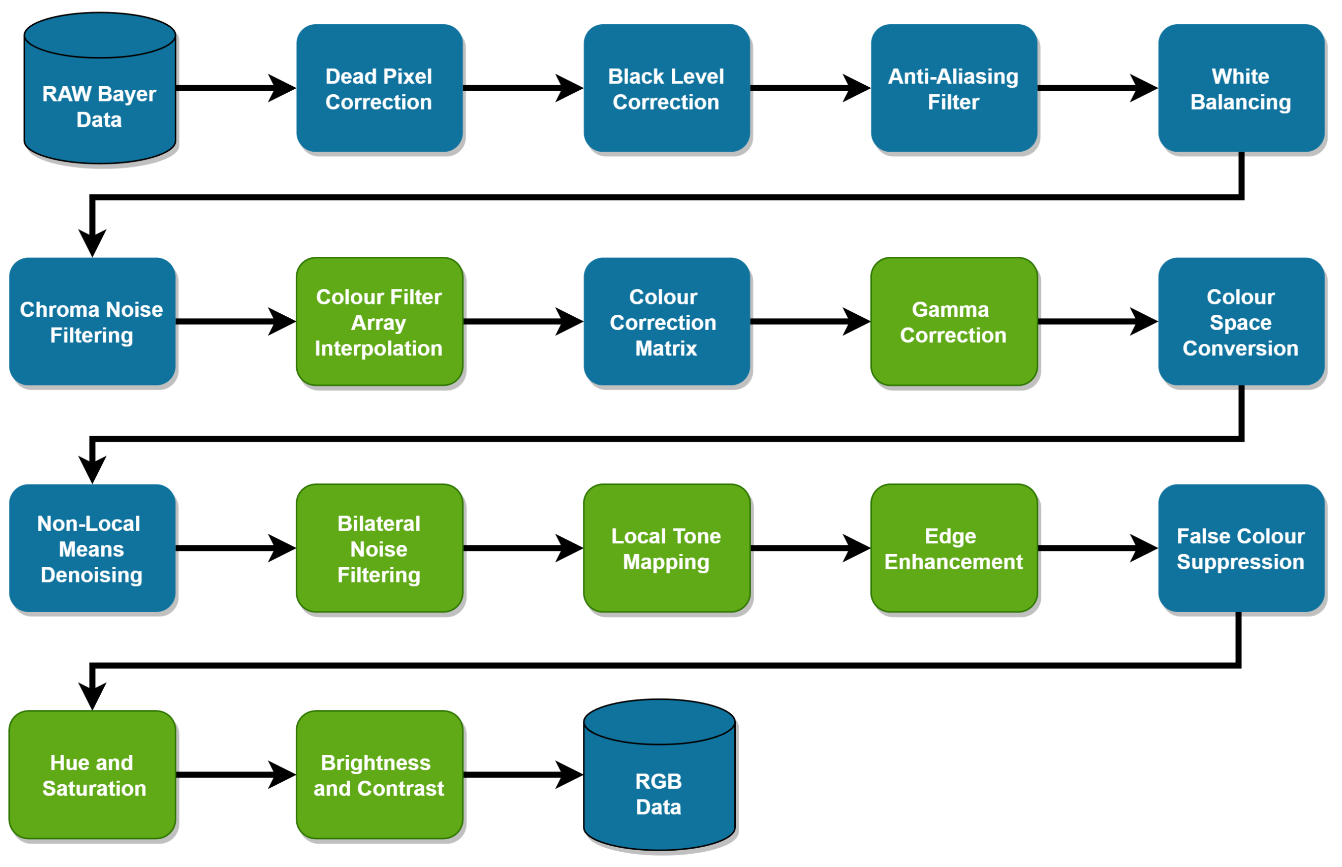
3.3. Software ISP
3.3.1. CFA Interpolation
3.3.2. Gamma Correction
3.3.3. Bilateral Noise Filtering
3.3.4. Local Tone Mapping
3.3.5. Edge Enhancement
3.3.6. Hue
3.3.7. Saturation
3.3.8. Global Contrast
3.4. Metrics
3.5. Analysis Pipeline
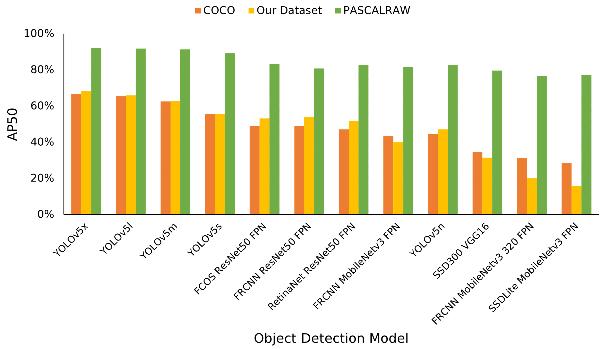
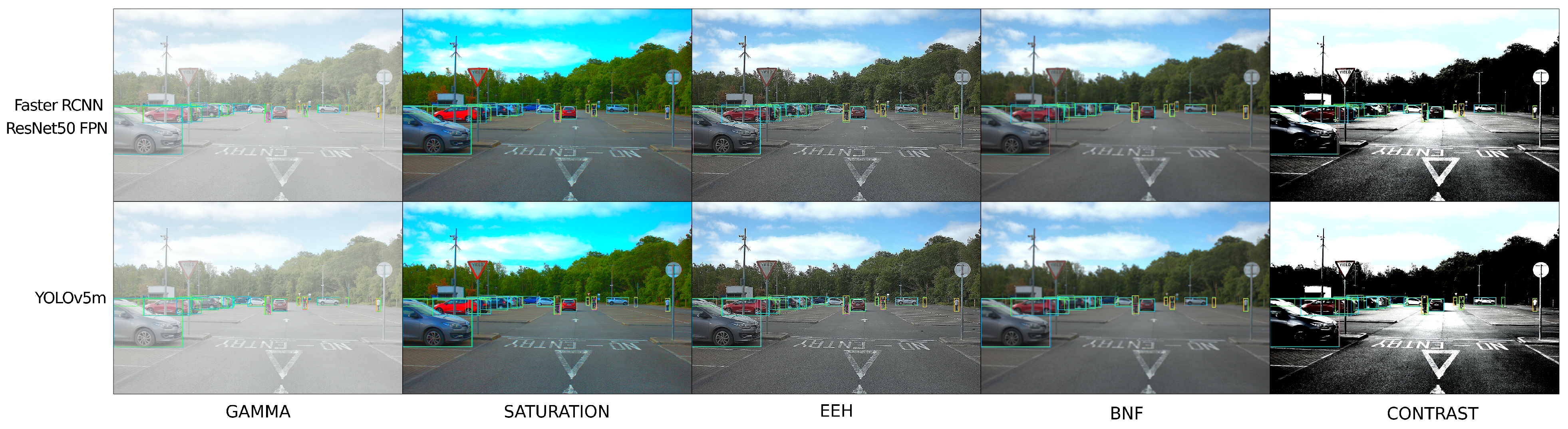
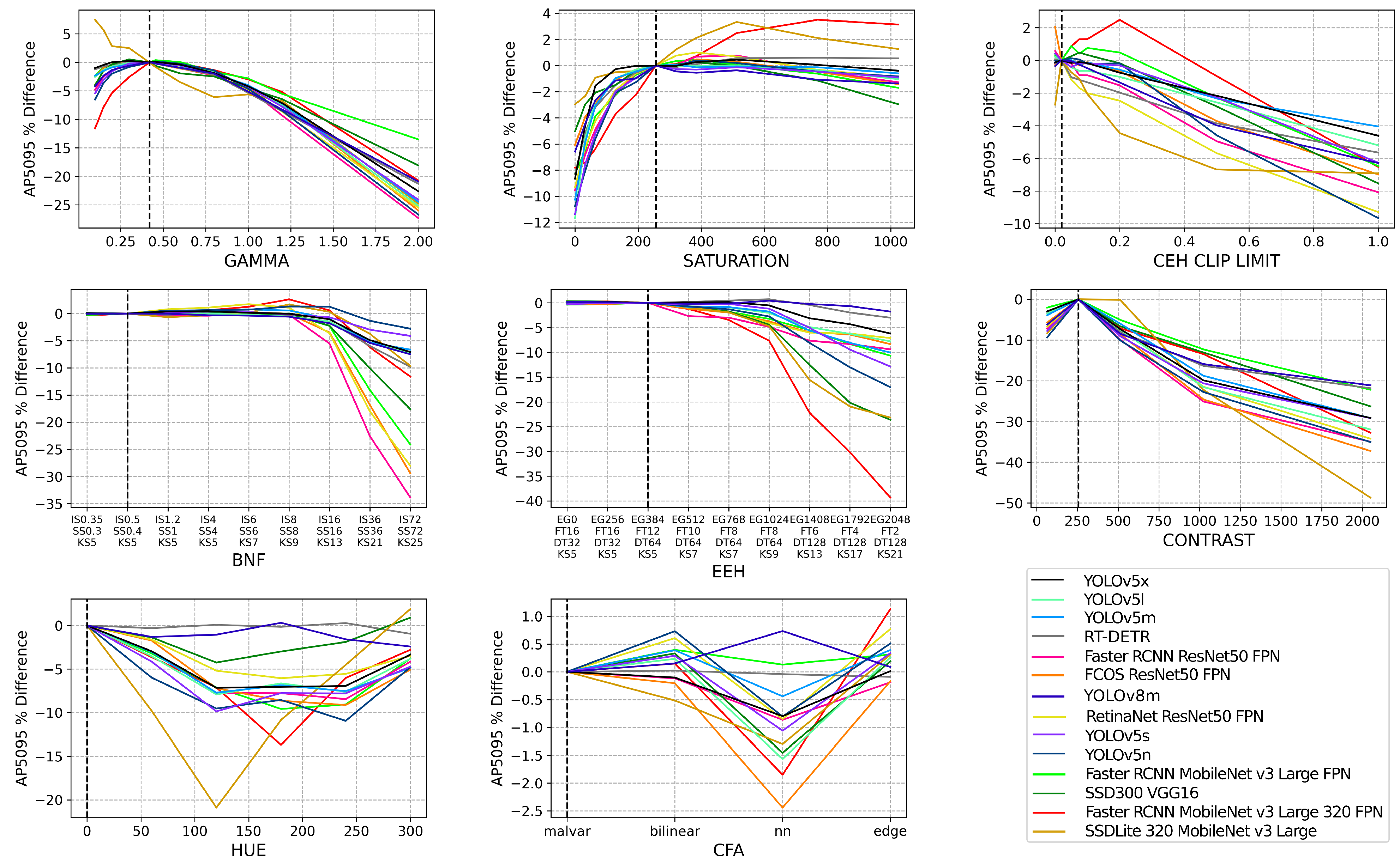
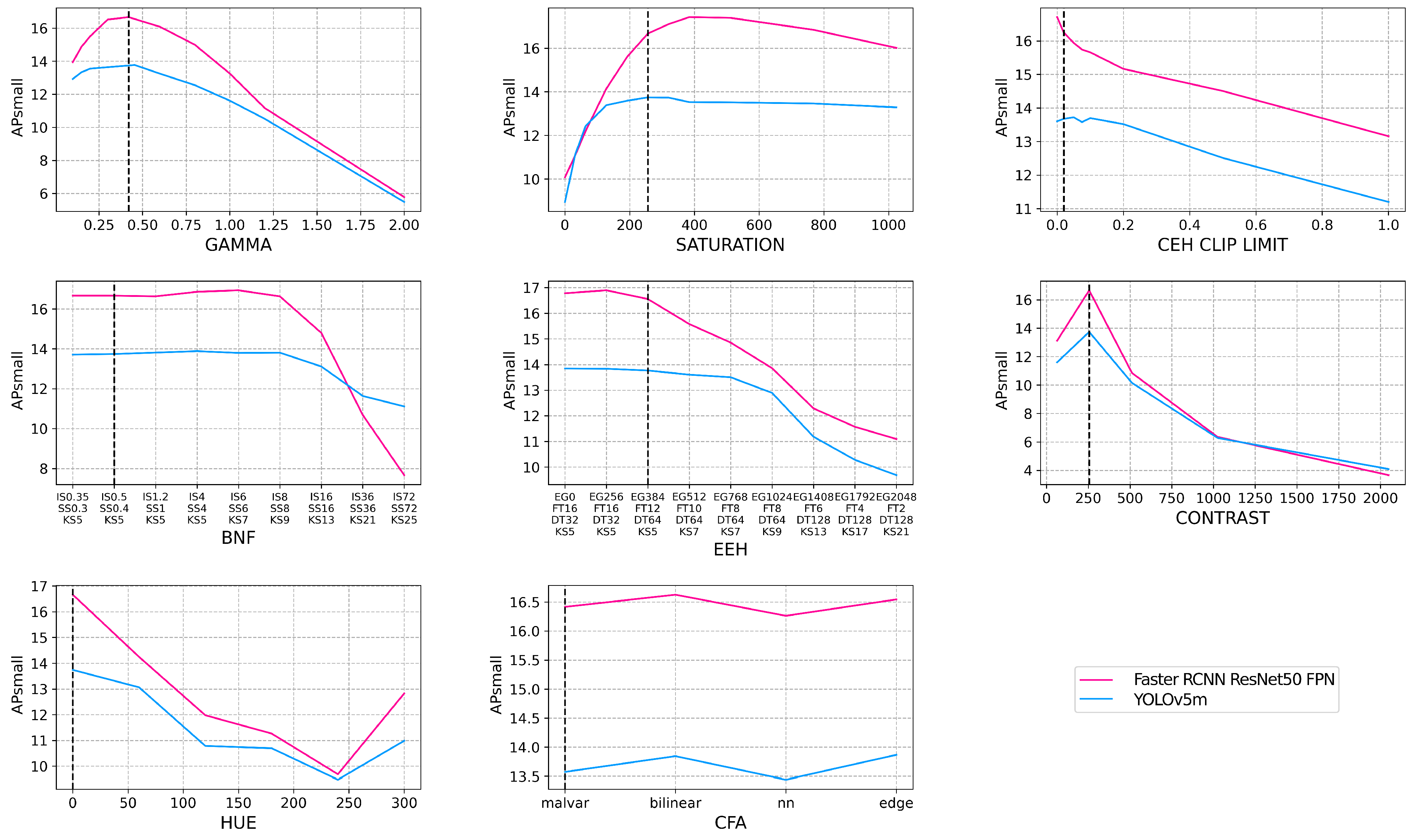
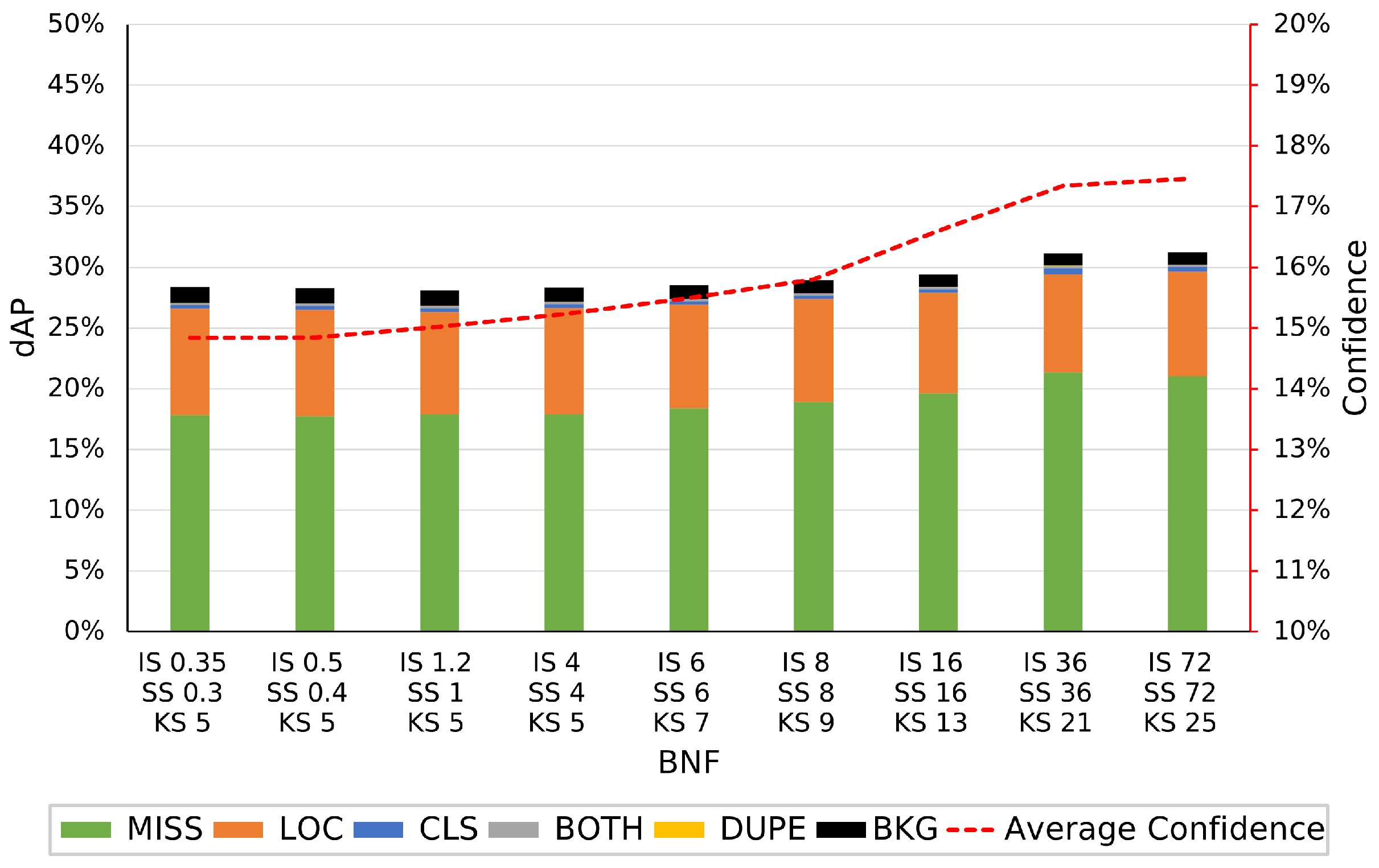
3.6. Results and Discussion
4. Data Augmentation with ISP Perturbation
4.1. Methodology
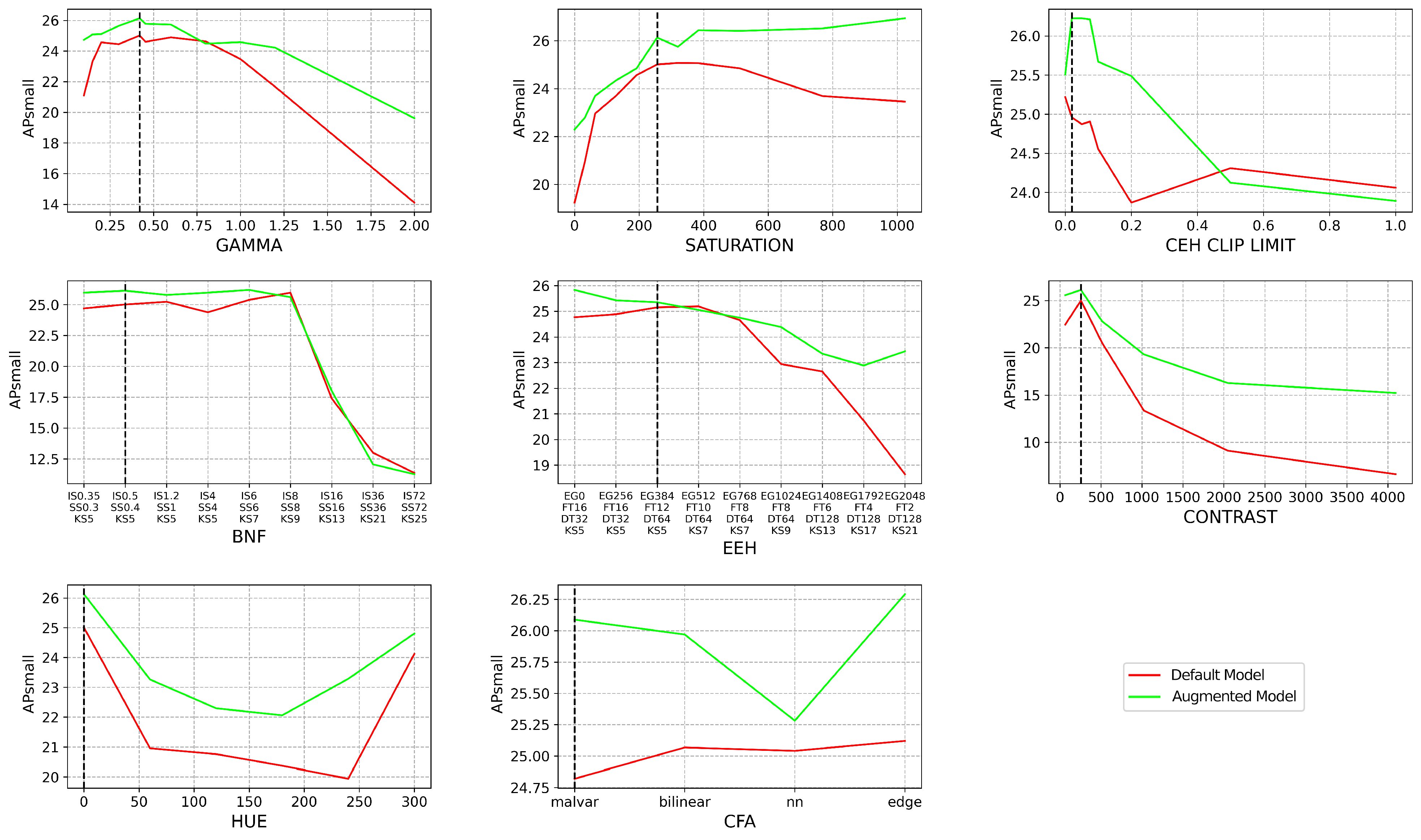
4.2. Results
5. Conclusions
Author Contributions
Funding
Data Availability Statement
Conflicts of Interest
References
- Zhao, Z.Q.; Zheng, P.; Xu, S.T.; Wu, X. Object Detection with Deep Learning: A Review. IEEE Trans. Neural Networks Learn. Syst. 2019, 30, 3212–3232. [Google Scholar] [CrossRef] [PubMed]
- Zhu, H.; Wei, H.; Li, B.; Yuan, X.; Kehtarnavaz, N. A Review of Video Object Detection: Datasets, Metrics and Methods. Appl. Sci. 2020, 10, 7834. [Google Scholar] [CrossRef]
- Chen, Y.; Xie, Y.; Song, L.; Chen, F.; Tang, T. A Survey of Accelerator Architectures for Deep Neural Networks. Engineering 2020, 6, 264–274. [Google Scholar] [CrossRef]
- Mishra, P.; Saroha, G. A Study on Video Surveillance System for Object Detection and Tracking. In Proceedings of the 2016 3rd International Conference on Computing for Sustainable Global Development (INDIACom), New Delhi, India, 16–18 March 2016. [Google Scholar]
- Wang, X.; Li, B.; Ma, H.; Luo, M. A fast quantity and position detection method based on monocular vision for a workpieces counting and sorting system. In Proceedings of the 2019 Chinese Control Conference (CCC), Guangzhou, China, 27–30 July 2019; pp. 7906–7911. [Google Scholar] [CrossRef]
- Haugaløkken, B.O.A.; Skaldebø, M.B.; Schjølberg, I. Monocular vision-based gripping of objects. Robot. Auton. Syst. 2020, 131, 103589. [Google Scholar] [CrossRef]
- Li, P.; Zhao, H. Monocular 3D object detection using dual quadric for autonomous driving. Neurocomputing 2021, 441, 151–160. [Google Scholar] [CrossRef]
- Yu, F.; Chen, H.; Wang, X.; Xian, W.; Chen, Y.; Liu, F.; Madhavan, V.; Darrell, T. BDD100K: A Diverse Driving Dataset for Heterogeneous Multitask Learning. In Proceedings of the IEEE Conference on Computer Vision and Pattern Recognition (CVPR), Seattle, WA, USA, 13–19 June 2020. [Google Scholar]
- Lin, T.Y.; Maire, M.; Belongie, S.; Bourdev, L.; Girshick, R.; Hays, J.; Perona, P.; Ramanan, D.; Zitnick, C.L.; Dollár, P. Microsoft COCO: Common Objects in Context. arXiv 2015, arXiv:1405.0312. [Google Scholar] [CrossRef]
- Mosleh, A.; Sharma, A.; Onzon, E.; Mannan, F.; Robidoux, N.; Heide, F. Hardware-in-the-Loop End-to-End Optimization of Camera Image Processing Pipelines. In Proceedings of the 2020 IEEE/CVF Conference on Computer Vision and Pattern Recognition (CVPR), Seattle, WA, USA, 13–19 June 2020; pp. 7526–7535. [Google Scholar] [CrossRef]
- OpenISP: Image Signal Processor. Available online: https://github.com/cruxopen/openISP (accessed on 20 November 2023).
- Jueqin, Q. Fast-openisp: A Faster Re-Implementation of OpenISP. Available online: https://github.com/QiuJueqin/fast-openISP (accessed on 20 November 2023).
- Gao, X.; Lu, W.; Tao, D.; Li, X. Image quality assessment and human visual system. In Proceedings of the Visual Communications and Image Processing, Huangshan, China, 11 July 2010; Frossard, P., Li, H., Wu, F., Girod, B., Li, S., Wei, G., Eds.; International Society for Optics and Photonics, SPIE: Bellingham, WA, USA, 2010; Volume 7744, p. 77440Z. [Google Scholar] [CrossRef]
- Buckler, M.; Jayasuriya, S.; Sampson, A. Reconfiguring the Imaging Pipeline for Computer Vision. arXiv 2017, arXiv:1705.04352. [Google Scholar] [CrossRef]
- Kim, S.J.; Lin, H.T.; Lu, Z.; Süsstrunk, S.; Lin, S.; Brown, M.S. A New In-Camera Imaging Model for Color Computer Vision and Its Application. IEEE Trans. Pattern Anal. Mach. Intell. 2012, 34, 2289–2302. [Google Scholar] [CrossRef]
- Uss, M.L.; Vozel, B.; Lukin, V.V.; Chehdi, K. Image informative maps for component-wise estimating parameters of signal-dependent noise. J. Electron. Imaging 2013, 22, 013019. [Google Scholar] [CrossRef]
- Yahiaoui, L.; Horgan, J.; Yogamani, S.; Eising, C.; Deegan, B. Impact analysis and tuning strategies for camera Image Signal Processing parameters in Computer Vision. In Proceedings of the 20th Irish Machine Vision and Image Processing Conference, Belfast, Ireland, 29–31 August 2018. [Google Scholar]
- Yahiaoui, L.; Horgan, J.; Deegan, B.; Yogamani, S.; Hughes, C.; Denny, P. Overview and Empirical Analysis of ISP Parameter Tuning for Visual Perception in Autonomous Driving. J. Imaging 2019, 5, 78. [Google Scholar] [CrossRef]
- Hansen, N. The CMA Evolution Strategy: A Tutorial. arXiv 2016, arXiv:1604.00772. [Google Scholar] [CrossRef]
- Hansen, P.; Vilkin, A.; Khrustalev, Y.; Imber, J.; Hanwell, D.; Mattina, M.; Whatmough, P.N. ISP4ML: Understanding the Role of Image Signal Processing in Efficient Deep Learning Vision Systems. arXiv 2021, arXiv:1911.07954. [Google Scholar] [CrossRef]
- Robidoux, N.; Seo, D.e.; Ariza, F.; Garcia Capel, L.E.; Sharma, A.; Heide, F. End-to-end High Dynamic Range Camera Pipeline Optimization. In Proceedings of the 2021 IEEE/CVF Conference on Computer Vision and Pattern Recognition (CVPR), Nashville, TN, USA, 20–25 June 2021; pp. 6293–6303. [Google Scholar] [CrossRef]
- Bochkovskiy, A.; Wang, C.Y.; Liao, H.Y.M. YOLOv4: Optimal Speed and Accuracy of Object Detection. arXiv 2020, arXiv:2004.10934. [Google Scholar] [CrossRef]
- Yahiaoui, L.; Eising, C.; Horgan, J.; Deegan, B.; Denny, P.; Yogamani, S. Optimization of ISP parameters for object detection algorithms. Electron. Imaging 2019, 31, art00014. [Google Scholar] [CrossRef]
- Omid-Zohoor, A.; Ta, D.; Murmann, B. PASCALRAW: Raw image database for object detection. Available online: https://searchworks.stanford.edu/view/hq050zr7488 (accessed on 20 November 2023).
- Sekachev, B.; Manovich, N.; Zhiltsov, M.; Zhavoronkov, A.; Kalinin, D.; Hoff, B.; TOsmanov; Kruchinin, D.; Zankevich, A.; DmitriySidnev; et al. OpenCV/CVAT: V1.1.0; Github: San Francisco, CA, USA, 2020. [Google Scholar] [CrossRef]
- Jocher, G.; Chaurasia, A.; Stoken, A.; Borovec, J.; NanoCode012; Kwon, Y.; Xie, T.; Fang, J.; imyhxy; Michael, K.; et al. Ultralytics/YOLOv5: V6.1—TensorRT, TensorFlow Edge TPU and OpenVINO Export and Inference; Github: San Francisco, CA, USA, 2022. [Google Scholar] [CrossRef]
- TorchVision: PyTorch’s Computer Vision Library. 2016. Available online: https://github.com/pytorch/vision (accessed on 20 November 2023).
- Girshick, R.; Donahue, J.; Darrell, T.; Malik, J. Rich feature hierarchies for accurate object detection and semantic segmentation. arXiv 2014, arXiv:1311.2524. [Google Scholar]
- Uijlings, J.R.R.; van de Sande, K.E.A.; Gevers, T.; Smeulders, A.W.M. Selective Search for Object Recognition. Int. J. Comput. Vis. 2013, 104, 154–171. [Google Scholar] [CrossRef]
- Girshick, R. Fast R-CNN. arXiv 2015, arXiv:1504.08083. [Google Scholar] [CrossRef]
- Ren, S.; He, K.; Girshick, R.; Sun, J. Faster R-CNN: Towards Real-Time Object Detection with Region Proposal Networks. arXiv 2016, arXiv:1506.01497. [Google Scholar] [CrossRef]
- Redmon, J.; Divvala, S.; Girshick, R.; Farhadi, A. You Only Look Once: Unified, Real-Time Object Detection. In Proceedings of the 2016 IEEE Conference on Computer Vision and Pattern Recognition (CVPR), Las Vegas, NV, USA, 27–30 June 2016; pp. 779–788. [Google Scholar] [CrossRef]
- Redmon, J.; Farhadi, A. YOLO9000: Better, Faster, Stronger. In Proceedings of the 2017 IEEE Conference on Computer Vision and Pattern Recognition (CVPR), Honolulu, HI, USA, 21–26 July 2017; pp. 6517–6525. [Google Scholar] [CrossRef]
- Redmon, J.; Farhadi, A. YOLOv3: An Incremental Improvement. arXiv 2018, arXiv:1804.02767. [Google Scholar]
- Wang, C.Y.; Bochkovskiy, A.; Liao, H.Y.M. YOLOv7: Trainable bag-of-freebies sets new state-of-the-art for real-time object detectors. arXiv 2022, arXiv:2207.02696. [Google Scholar] [CrossRef]
- Jocher, G.; Chaurasia, A.; Qiu, J. Ultralytics YOLOv8. 2023. Available online: https://github.com/ultralytics/ultralytics (accessed on 20 November 2023).
- Liu, W.; Anguelov, D.; Erhan, D.; Szegedy, C.; Reed, S.E.; Fu, C.; Berg, A.C. SSD: Single Shot MultiBox Detector. In Proceedings of the 2016 ECCV European Conference on Computer Vision, 14th European Conference, Amsterdam, The Netherlands, 11–14 October 2016; pp. 21–37. [Google Scholar]
- Lin, T.Y.; Goyal, P.; Girshick, R.; He, K.; Dollár, P. Focal Loss for Dense Object Detection. arXiv 2018, arXiv:1708.02002. [Google Scholar] [CrossRef]
- Lin, T.Y.; Dollár, P.; Girshick, R.; He, K.; Hariharan, B.; Belongie, S. Feature Pyramid Networks for Object Detection. arXiv 2017, arXiv:1612.03144. [Google Scholar] [CrossRef]
- Tian, Z.; Shen, C.; Chen, H.; He, T. FCOS: Fully Convolutional One-Stage Object Detection. In Proceedings of the 2019 IEEE/CVF International Conference on Computer Vision (ICCV), Seoul, Republic of Korea, 27–2 November 2019; pp. 9626–9635. [Google Scholar] [CrossRef]
- Lv, W.; Zhao, Y.; Xu, S.; Wei, J.; Wang, G.; Cui, C.; Du, Y.; Dang, Q.; Liu, Y. DETRs Beat YOLOs on Real-time Object Detection. arXiv 2023, arXiv:2304.08069. [Google Scholar]
- Carion, N.; Massa, F.; Synnaeve, G.; Usunier, N.; Kirillov, A.; Zagoruyko, S. End-to-End Object Detection with Transformers. In Proceedings of the 2020 ECCV European Conference on Computer Vision, 16th European Conference, Glasgow, UK, 23–28 August 2020; pp. 213–229. [Google Scholar]
- PaddleClas. Available online: https://github.com/PaddlePaddle/PaddleClas (accessed on 20 November 2023).
- Schöberl, M.; Schnurrer, W.; Oberdörster, A.; Fössel, S.; Kaup, A. Dimensioning of optical birefringent anti-alias filters for digital cameras. In Proceedings of the 2010 IEEE International Conference on Image Processing, Hong Kong, China, 26–29 September 2010; pp. 4305–4308. [Google Scholar] [CrossRef]
- Li, X.; Gunturk, B.; Zhang, L. Image demosaicing: A systematic survey. In Proceedings of the Visual Communications and Image Processing 2008, San Jose, CA, USA, 28 January 2008; p. 68221J. [Google Scholar] [CrossRef]
- OpenCV: Open Computer Vision Library. 2000. Available online: https://opencv.org/ (accessed on 20 November 2023).
- sRGB IEC 61966-2-1:1999. Available online: https://webstore.iec.ch/publication/6169 (accessed on 20 November 2023).
- Wang, G.; Renshaw, D.; Denyer, P.; Lu, M. CMOS video cameras. In Proceedings of the Euro ASIC ’91, Paris, France, 27–31 May 1991; pp. 100–103. [Google Scholar] [CrossRef]
- EMVA Working Group EMVA Standard 1288. Available online: https://zenodo.org/records/3951558 (accessed on 20 November 2023).
- Tomasi, C.; Manduchi, R. Bilateral filtering for gray and color images. In Proceedings of the Sixth International Conference on Computer Vision (IEEE Cat. No.98CH36271), Bombay, India, 7 January 1998; pp. 839–846. [Google Scholar] [CrossRef]
- Chan, R.; Ho, C.W.; Nikolova, M. Salt-and-pepper noise removal by median-type noise detectors and detail-preserving regularization. IEEE Trans. Image Process. 2005, 14, 1479–1485. [Google Scholar] [CrossRef] [PubMed]
- Chang, S.; Yu, B.; Vetterli, M. Adaptive wavelet thresholding for image denoising and compression. IEEE Trans. Image Process. 2000, 9, 1532–1546. [Google Scholar] [CrossRef]
- Pizer, S.M.; Amburn, E.P.; Austin, J.D.; Cromartie, R.; Geselowitz, A.; Greer, T.; Romeny, B.t.H.; Zimmerman, J.B.; Zuiderveld, K. Adaptive histogram equalization and its variations. Comput. Vision, Graph. Image Process. 1987, 39, 355–368. [Google Scholar] [CrossRef]
- Polesel, A.; Ramponi, G.; Mathews, V. Image enhancement via adaptive unsharp masking. IEEE Trans. Image Process. 2000, 9, 505–510. [Google Scholar] [CrossRef]
- Fairchild, M.D. Color Appearance Models: CIECAM02 and Beyond. In Proceedings of the Tutorial Slides for IS&T/SID 12th Color Imaging Conference, Scottsdale, AZ, USA, 9–12 November 2004. [Google Scholar]
- Everingham, M.; Van Gool, L.; Williams, C.K.I.; Winn, J.; Zisserman, A. The PASCAL Visual Object Classes Challenge 2012 (VOC2012) Results. Available online: http://host.robots.ox.ac.uk/pascal/VOC/ (accessed on 20 November 2023).
- Bolya, D.; Foley, S.; Hays, J.; Hoffman, J. TIDE: A General Toolbox for Identifying Object Detection Errors. arXiv 2020, arXiv:2008.08115. [Google Scholar] [CrossRef]
- Molloy, D. ISP Object Detection Benchmark. Available online: https://zenodo.org/records/7802651 (accessed on 20 November 2023).
- Shorten, C.; Khoshgoftaar, T.M. A survey on Image Data Augmentation for Deep Learning. J. Big Data 2019, 6, 60. [Google Scholar] [CrossRef]


| Class | # Objects | |
|---|---|---|
| Our Dataset | Pascalraw | |
| Person | 2435 | 4077 |
| Bicycle | 604 | 708 |
| Car | 5117 | 1765 |
| Total | 8156 | 6550 |
| Investigated Object Detection Models | ||||
|---|---|---|---|---|
| Model | Backbone | Stages | Params (M) | Year |
| FCOS | ResNet50 FPN | 1 | 32.3 | 2019 |
| Faster RCNN | ResNet50 FPN | 2 | 41.8 | 2016 |
| RetinaNet | ResNet50 FPN | 1 | 34 | 2017 |
| Faster RCNN | MobileNetv3 FPN | 2 | 19.4 | 2019 |
| Faster RCNN | MobileNetv3 320 FPN | 2 | 19.4 | 2019 |
| SSDLite | MobileNetv3 FPN | 1 | 3.4 | 2019 |
| SSD300 | VGG16 | 1 | 35.6 | 2015 |
| YOLOv5x | CSP | 1 | 86.7 | 2020 |
| YOLOv5l | CSP | 1 | 46.5 | 2020 |
| YOLOv5m | CSP | 1 | 21.2 | 2020 |
| YOLOv5s | CSP | 1 | 7.2 | 2020 |
| YOLOv5n | CSP | 1 | 1.9 | 2020 |
| YOLOv8m | CSP | 1 | 25.9 | 2023 |
| RT-DETR | HGNetv2 | 2 | 32 | 2023 |
| ISP Block | Parameters | Minimum | Default | Maximum |
|---|---|---|---|---|
| CFA Interpolation | Malvar Bilinear Nearest Neighbor Edge-Aware | - | Malvar | - |
| Gamma Correction | Exponent | 0.1 | 0.45 | 2.0 |
| Bilateral Noise Filtering | Intensity Sigma Spatial Sigma Kernel Size | 0.35 0.3 5.0 | 0.5 0.4 5.0 | 72.0 72.0 25.0 |
| Local Tone Mapping | Clip Limit | 0.0 | 0.02 | 1.0 |
| Edge Enhancement | Edge Gain Flat Threshold Delta Threshold Kernel Size | 0 16 32 5 | 384 12 64 5 | 2048 2 128 21 |
| Hue | Hue Angle | 0 | 0 | 300 |
| Saturation | Saturation Factor | 0 | 256 | 1024 |
Disclaimer/Publisher’s Note: The statements, opinions and data contained in all publications are solely those of the individual author(s) and contributor(s) and not of MDPI and/or the editor(s). MDPI and/or the editor(s) disclaim responsibility for any injury to people or property resulting from any ideas, methods, instructions or products referred to in the content. |
© 2023 by the authors. Licensee MDPI, Basel, Switzerland. This article is an open access article distributed under the terms and conditions of the Creative Commons Attribution (CC BY) license (https://creativecommons.org/licenses/by/4.0/).
Share and Cite
Molloy, D.; Deegan, B.; Mullins, D.; Ward, E.; Horgan, J.; Eising, C.; Denny, P.; Jones, E.; Glavin, M. Impact of ISP Tuning on Object Detection. J. Imaging 2023, 9, 260. https://doi.org/10.3390/jimaging9120260
Molloy D, Deegan B, Mullins D, Ward E, Horgan J, Eising C, Denny P, Jones E, Glavin M. Impact of ISP Tuning on Object Detection. Journal of Imaging. 2023; 9(12):260. https://doi.org/10.3390/jimaging9120260
Chicago/Turabian StyleMolloy, Dara, Brian Deegan, Darragh Mullins, Enda Ward, Jonathan Horgan, Ciaran Eising, Patrick Denny, Edward Jones, and Martin Glavin. 2023. "Impact of ISP Tuning on Object Detection" Journal of Imaging 9, no. 12: 260. https://doi.org/10.3390/jimaging9120260
APA StyleMolloy, D., Deegan, B., Mullins, D., Ward, E., Horgan, J., Eising, C., Denny, P., Jones, E., & Glavin, M. (2023). Impact of ISP Tuning on Object Detection. Journal of Imaging, 9(12), 260. https://doi.org/10.3390/jimaging9120260