

Numerical Simulation of a Bird-Inspired UAV Which Turns Without a Tail Through Proverse Yaw †

 and
and
Abstract
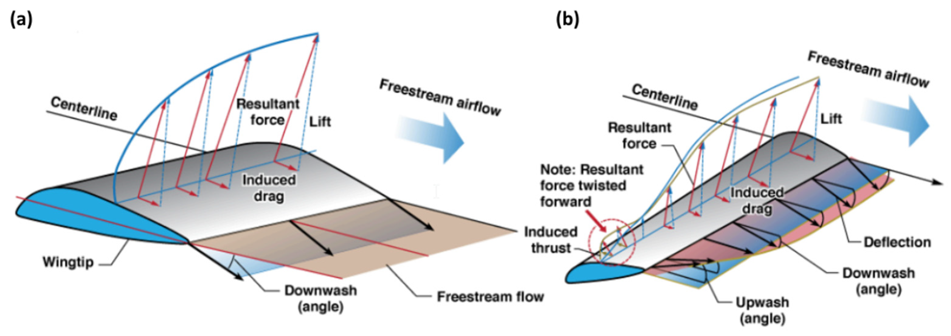
1. Introduction
2. Numerical Methods
2.1. Solver
2.2. Grid Motion for 6DOFs Simulations
2.3. Grid Convergence Study
2.4. Validations
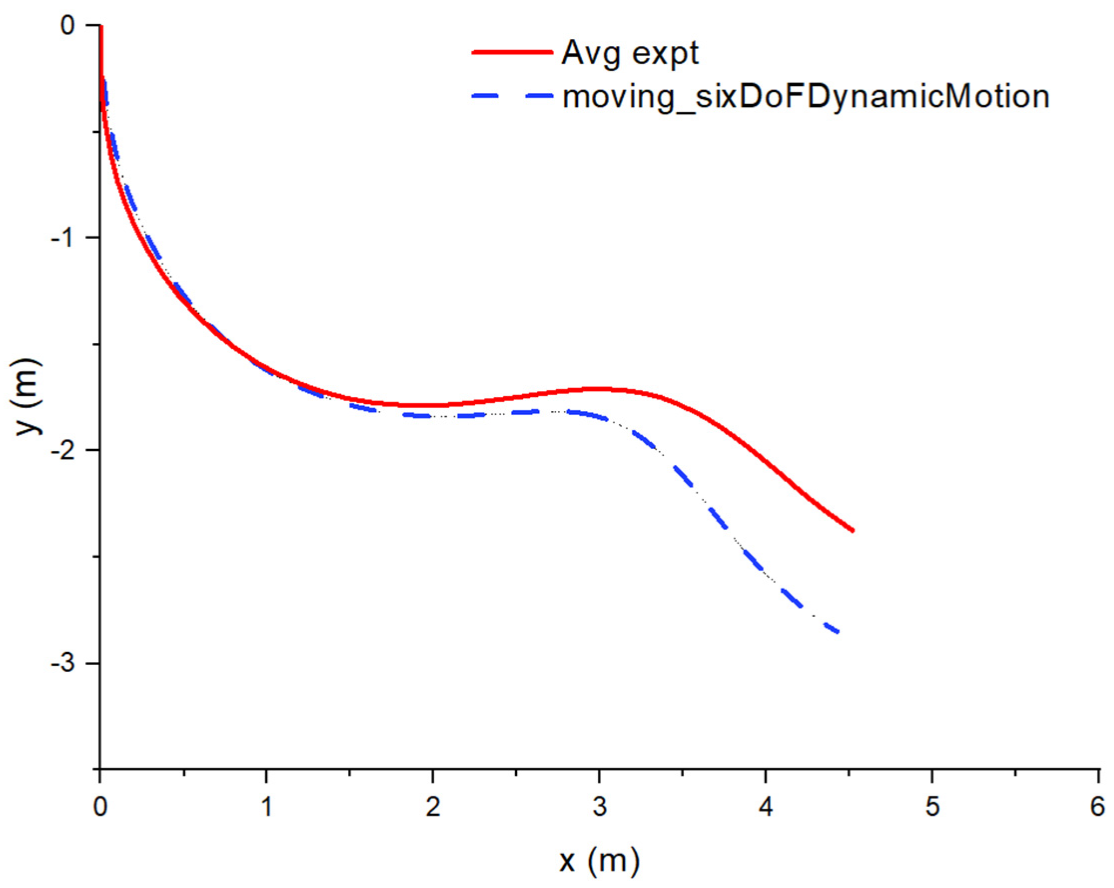
2.5. Experimental Validation of the Moving_sixDoFDynamicMotion Solver
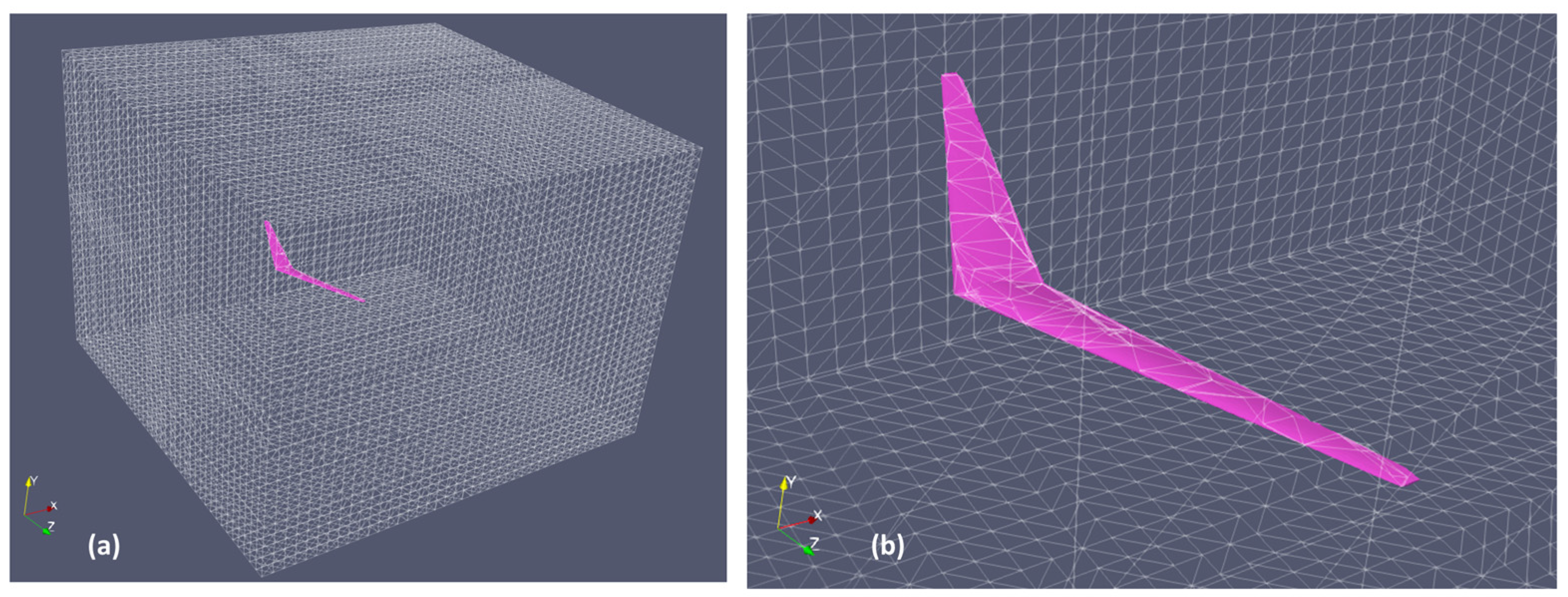
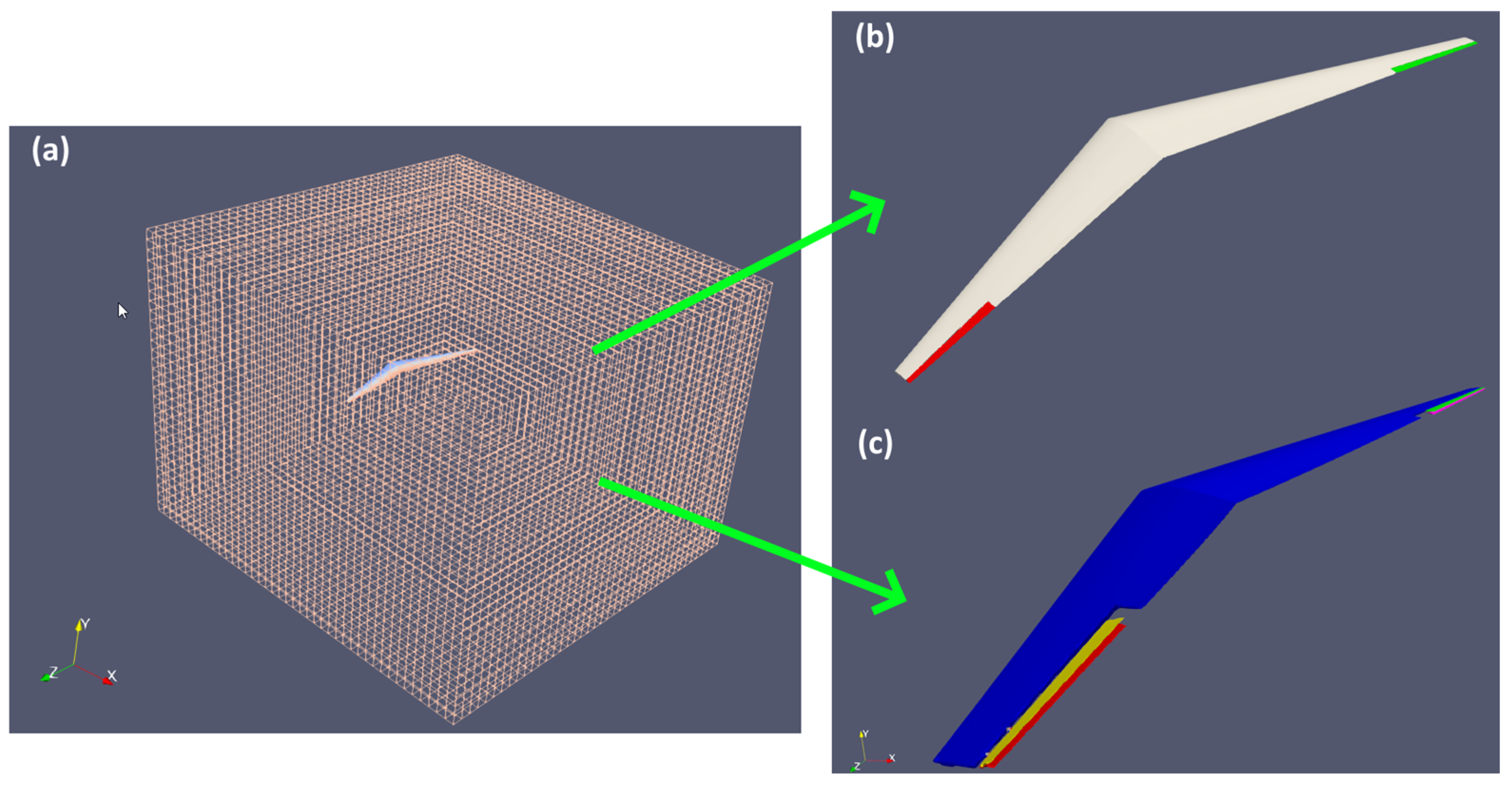
2.6. Simulation Setup
3. Research Methodology
3.1. Validation of Proverse Yaw Through Full 6DOFs Simulation
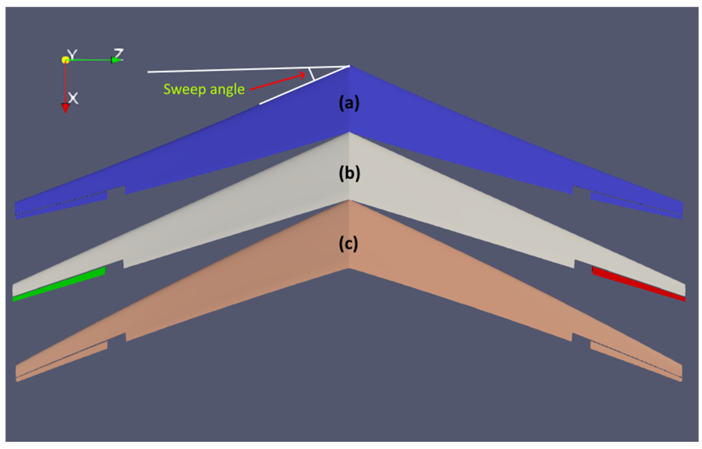
3.2. Effect of Sweep Angle on Proverse Yaw
4. Results and Discussions
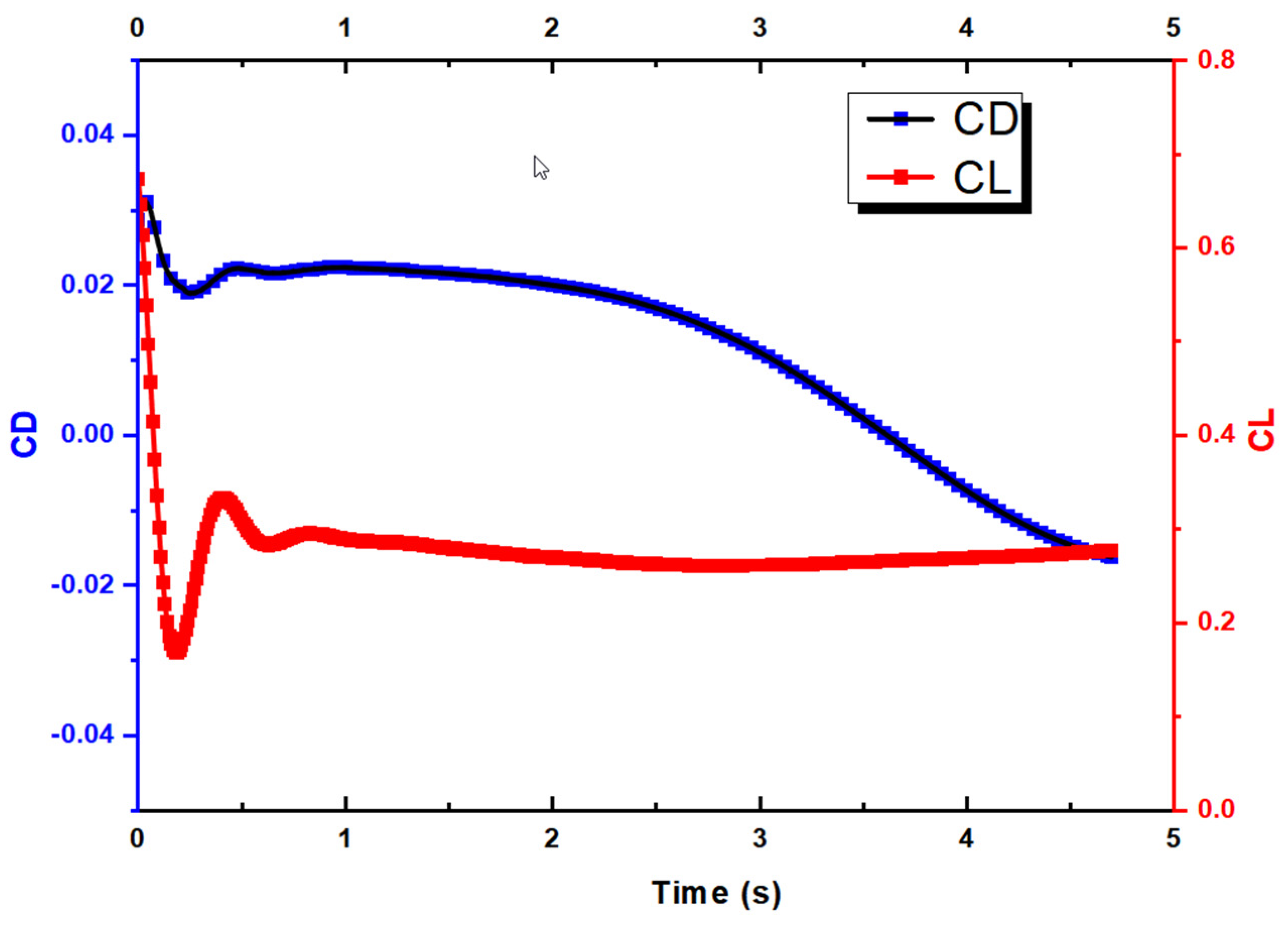
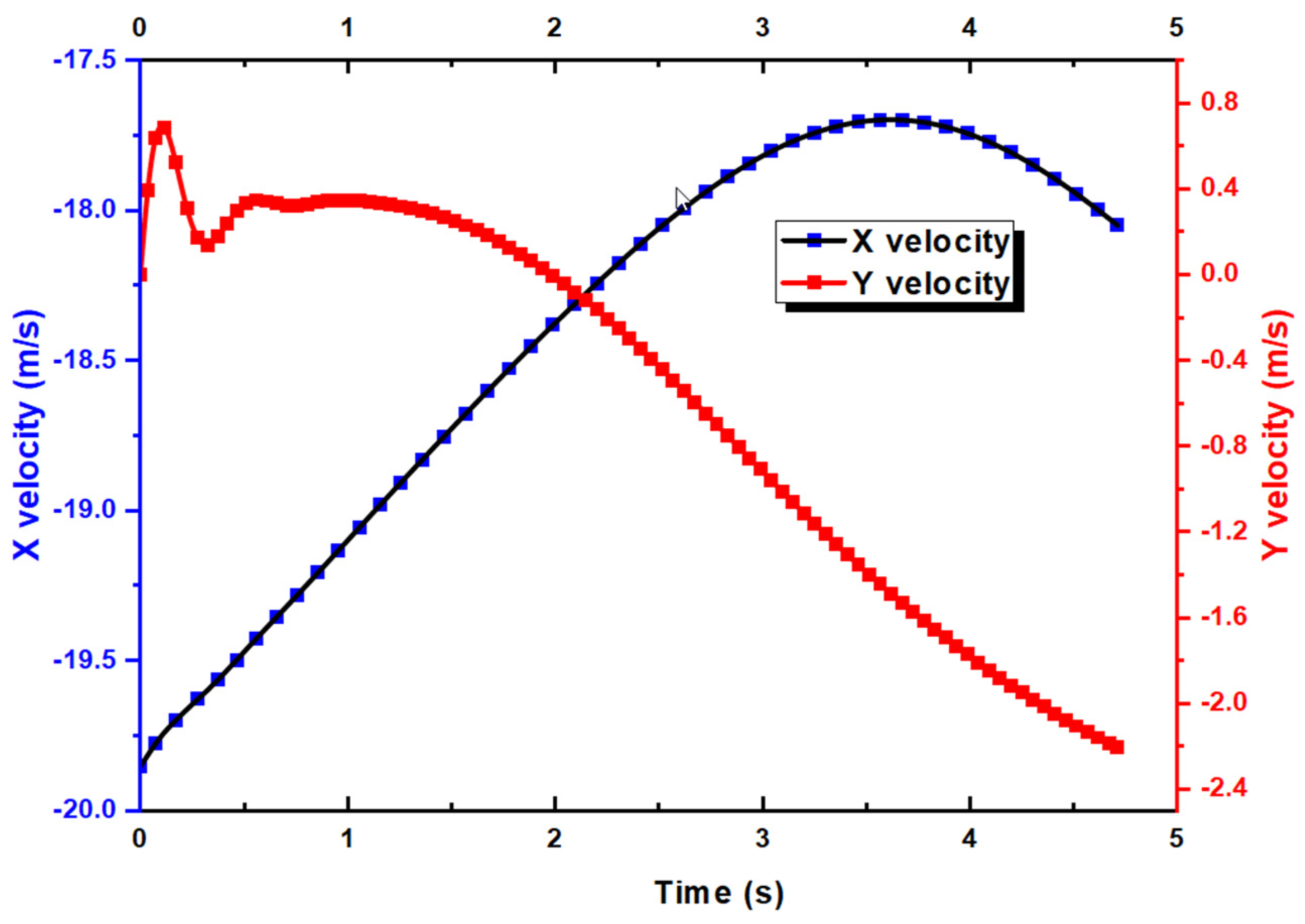
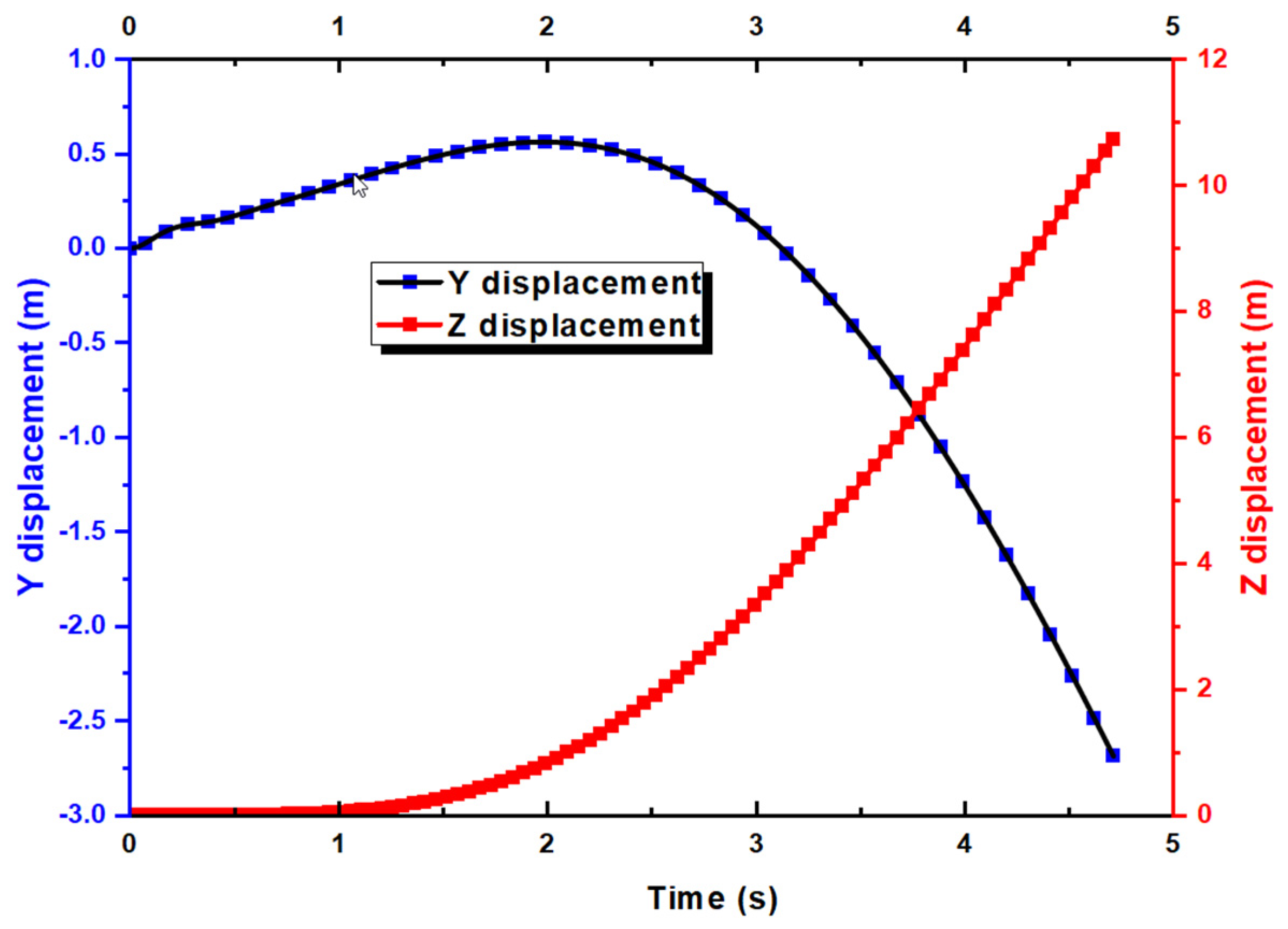
4.1. Full 6DOFs Simulation of UAV for Proverse Yaw Validation
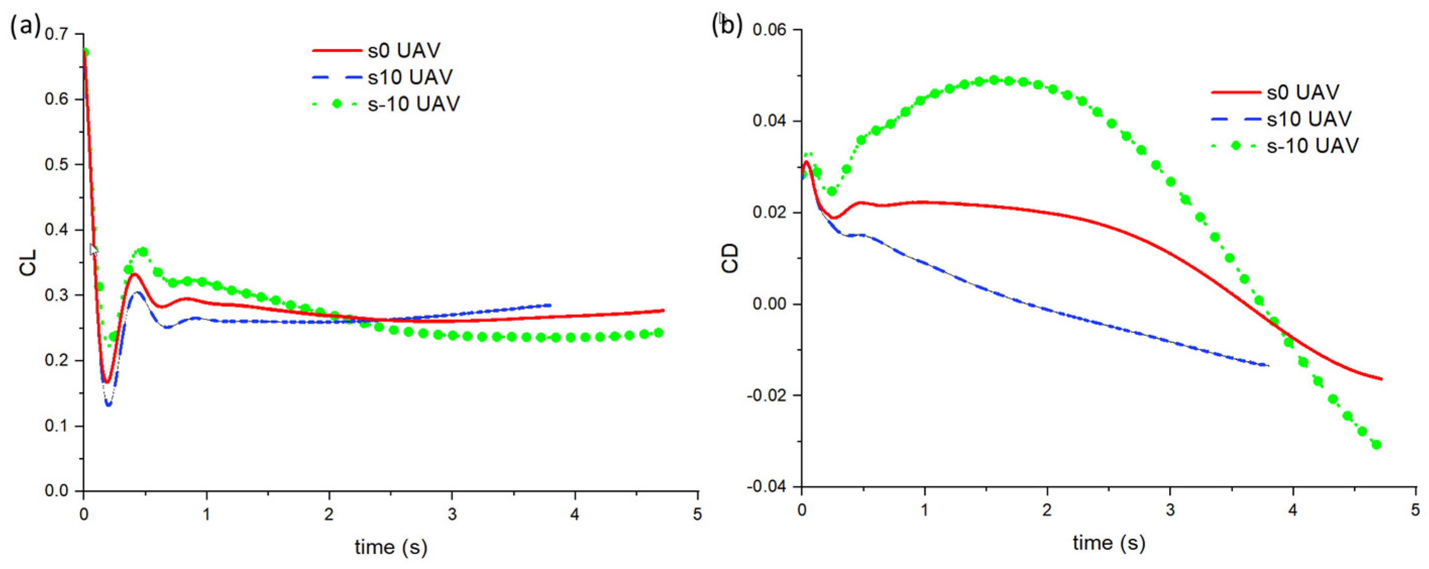
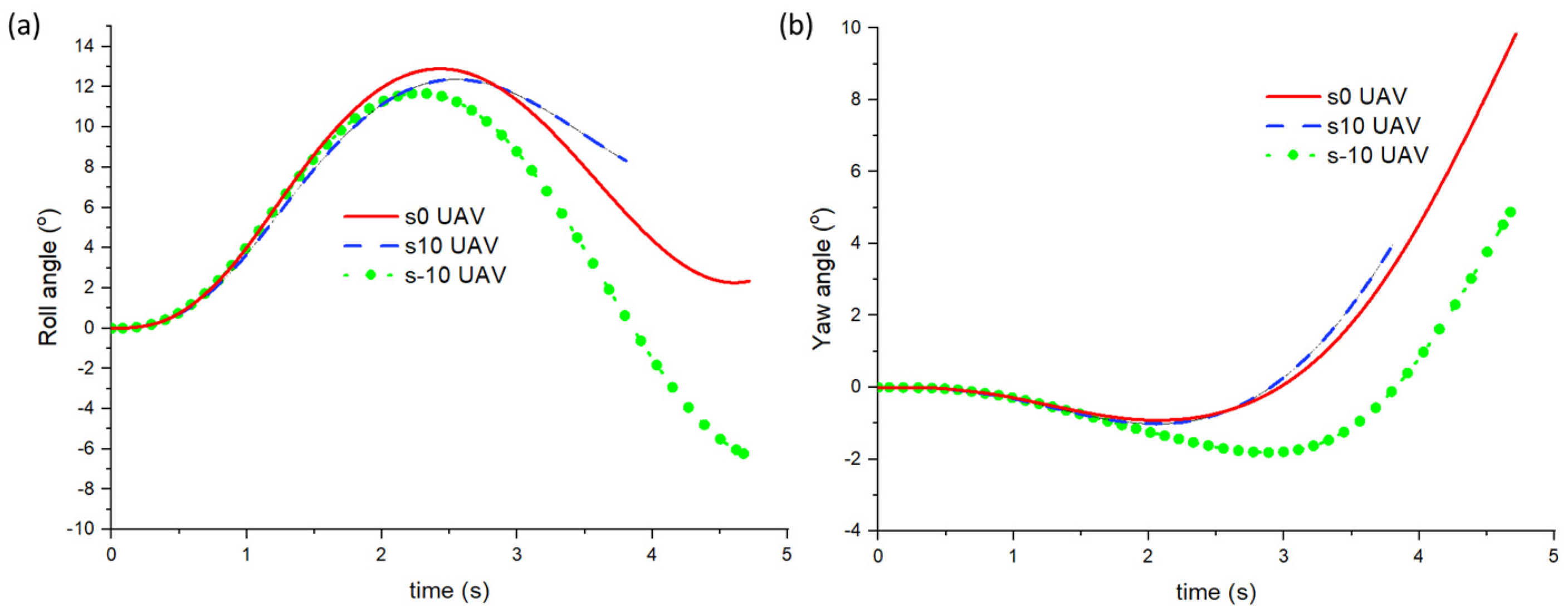
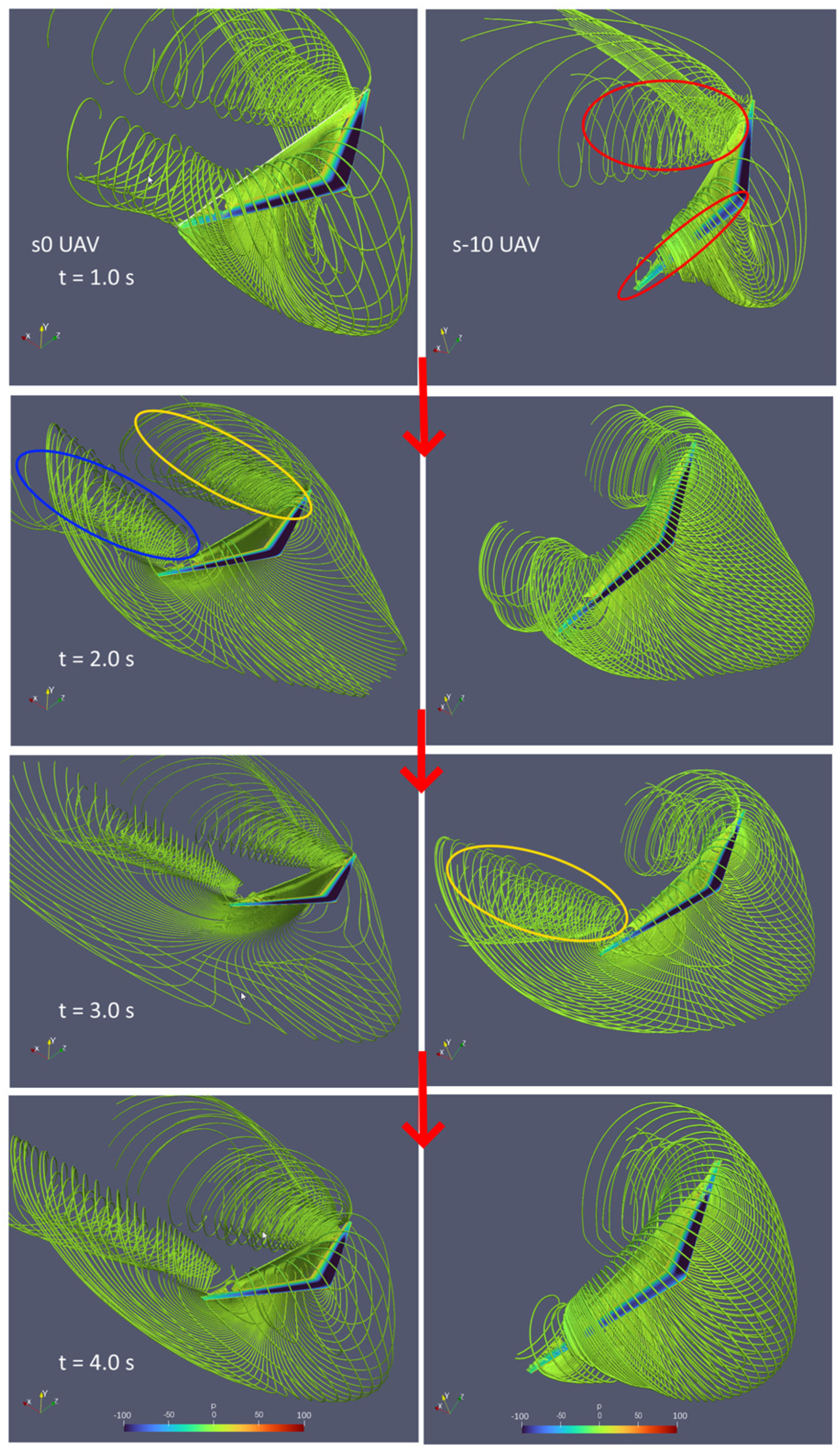
4.2. Effect of Sweep Angle on Proverse Yaw and UAV’s Performance
5. Conclusions
Author Contributions
Funding
Institutional Review Board Statement
Informed Consent Statement
Data Availability Statement
Acknowledgments
Conflicts of Interest
Abbreviations
| 6DOF | 6 degree-of-freedom |
| CD | Drag coefficient |
| CL | Lift coefficient |
| OF | OpenFOAM |
References
- Prandtl, L. Tragflügeltheorie. I. Mitteilung. Nachrichten Ges. Wiss. Göttingen Math.-Phys. Kl. 1918, 1918, 451–477. [Google Scholar]
- Shen, Y.; Zhang, S.; Huang, W.; Shang, C.; Sun, T.; Shi, Q. Characterization of Wing Kinematics by Decoupling Joint Movement in the Pigeon. Biomimetics 2024, 9, 555. [Google Scholar] [CrossRef]
- Bishay, P.; Rini, A.; Brambila, M.; Niednagel, P.; Eghdamzamiri, J.; Yousefi, H.; Herrera, J.; Saad, Y.; Bertuch, E.; Black, C.; et al. CGull: A Non-Flapping Bioinspired Composite Morphing Drone. Biomimetics 2024, 9, 527. [Google Scholar] [CrossRef]
- Prandtl, L. Über Tragflügel Kleinsten Induzierten Widerstandes. Z. Flugtecknik Mot. 1933, 24, 305–306. [Google Scholar]
- Bowers, A.H. On Wings of the Minimum Induced Drag—Spanload Implications for Aircraft and Birds; NASA: Washington, DC, USA, 2016.
- Newton, L.J. Stability and Control Derivative Estimation for the Bell-Shaped Lift Distribution. In Proceedings of the AIAA Scitech 2019 Forum, San Diego, CA, USA, 7–11 January 2019; American Institute of Aeronautics and Astronautics: Reston, VA, USA, 2019. [Google Scholar]
- Hunsaker, D.F.; Montgomery, Z.S.; Joo, J.J. Adverse-Yaw Control During Roll for a Class of Optimal Lift Distributions. AIAA J. 2020, 58, 2909–2920. [Google Scholar] [CrossRef]
- Yoo, S. Computational Fluid Dynamics Analysis of the Stall Characteristics of a Wing Designed Based on Prandtl’s Minimum Induced Drag. In Proceedings of the 2018 Applied Aerodynamics Conference, Atlanta, GA, USA, 25–29 June 2018; American Institute of Aeronautics and Astronautics: Reston, VA, USA, 2018. [Google Scholar]
- Richter, J.; Hainline, K.; Agarwal, R.K. Examination of Proverse Yaw in Bell-Shaped Spanload Aircraft; Mechanical Engineering and Materials Science Independent Study. 91; Washington University in St. Louis: St. Louis, MO, USA, 2019. [Google Scholar]
- Weekley, S. Design and Analysis of Bellwether—A Flying Wing Featuring the Bell-Shaped Spanload. Master’s Thesis, Oklahoma State University, Stillwater, OK, USA, 2021. Available online: https://www.proquest.com/openview/910b06882c396ee577d9c1bc16ceb88a/1?cbl=18750&diss=y&pq-origsite=gscholar (accessed on 31 January 2025).
- Kelly, C. Project Monarch—The Application of Ludwig Prandtl’s Bell-Curve Span Loading to a Straight, High Performance Sailplane Wing. Master’s Thesis, Oklahoma State University, Stillwater, OK, USA, 2021. Available online: https://www.proquest.com/openview/f0e48878ef8d820564d4b5a5d060c3a8/1?cbl=18750&diss=y&pq-origsite=gscholar (accessed on 31 January 2025).
- Weller, H.G.; Tabor, G.; Jasak, H.; Fureby, C. A Tensorial Approach to Computational Continuum Mechanics Using Object-Oriented Techniques. Comput. Phys. 1998, 12, 620–631. [Google Scholar] [CrossRef]
- Issa, R.I. Solution of the Implicitly Discretised Fluid Flow Equations by Operator-Splitting. J. Comput. Phys. 1986, 62, 40–65. [Google Scholar] [CrossRef]
- Patankar, S.V.; Spalding, D.B. A Calculation Procedure For Heat, Mass And Momentum Transfer In Three-Dimensional Parabolic Flows. Int. J. Heat Mass Transf. 1972, 15, 1787–1806. [Google Scholar] [CrossRef]
- Petersson, N.A. Hole-Cutting for Three-Dimensional Overlapping Grids. SIAM J. Sci. Comput. 1999, 21, 646–665. [Google Scholar] [CrossRef]
- Kumar, A. sixDoFDynamicMotion 2019. Available online: https://github.com/krajit/sixDoFDynamicMotion (accessed on 31 January 2025).
- Bowers, A.H. Experimental Flight Validation of the Prandtl 1933 Bell Spanload; NASA/TM–20210014683; NASA: Washington, DC, USA, 2021.
- Tay, W.-B.; Chan, W.-L.; Chong, R.-O.; Tay Chien-Ming, J. Framework for Numerical 6DOF Simulation with Focus on a Wing Deforming UAV in Perch Landing. Aerospace 2024, 11, 657. [Google Scholar] [CrossRef]
- Tay, W.B.; Chong, R.O.; Tay, J.C.M. Numerical Validation and Sensitivity Tests of a Model Aircraft in Free Fall. In Proceedings of the AIAA SCITECH 2024 Forum, Orlando, FL, USA, 8–12 January 2024; American Institute of Aeronautics and Astronautics: Reston, VA, USA, 2024. [Google Scholar]
- Hammer, P.R.; Garmann, D.J. Simulations of a Bell-Shaped Span-Loaded Swept Wing. In Proceedings of the AIAA SCITECH 2023 Forum, National Harbor, MD, USA, 23–27 January 2023; American Institute of Aeronautics and Astronautics: Reston, VA, USA, 2023. [Google Scholar]


| Grid Size (Millions) | CD | CL |
|---|---|---|
| 3.9 | 0.61 | 0.54 |
| 6.4 | 0.031 | 0.66 |
| 12.1 | 0.031 | 0.69 |
| 22.5 | 0.029 | 0.71 |
| Variable | Bowers et al. [17] Wind Tunnel at AoA = 0° | Current at AoA = 7° |
|---|---|---|
| CL | 0.71 | 0.71 |
| CD | 0.043 | 0.29 |
| Center of mass | (0, 0, 0) m |
| Mass | 6.58 kg |
| Roll inertia | 7.355 kgm2 |
| Yaw inertia | 7.888 kgm2 |
| Pitch inertia | 0.368 kgm2 |
| Wingspan | 3.749 m |
| Centerline chord length (reference length) | 0.4 m |
| velocity | (19.85, 0, 0) m/s |
| Planform area (reference area) | 0.94 m2 |
| Dihedral angle | 2.5° |
| Leading edge sweep | 24° at the nose |
| Aileron location | Located in the outboard 14% of each wing, in the trailing 25% of the chord |
Disclaimer/Publisher’s Note: The statements, opinions and data contained in all publications are solely those of the individual author(s) and contributor(s) and not of MDPI and/or the editor(s). MDPI and/or the editor(s) disclaim responsibility for any injury to people or property resulting from any ideas, methods, instructions or products referred to in the content. |
© 2025 by the authors. Licensee MDPI, Basel, Switzerland. This article is an open access article distributed under the terms and conditions of the Creative Commons Attribution (CC BY) license (https://creativecommons.org/licenses/by/4.0/).
Share and Cite
Tay, W.-B.; Chong, T.S.J.-S.; Chan, J.-Q.; Chan, W.-L.; Khoo, B.-C. Numerical Simulation of a Bird-Inspired UAV Which Turns Without a Tail Through Proverse Yaw. Biomimetics 2025, 10, 253. https://doi.org/10.3390/biomimetics10040253
Tay W-B, Chong TSJ-S, Chan J-Q, Chan W-L, Khoo B-C. Numerical Simulation of a Bird-Inspired UAV Which Turns Without a Tail Through Proverse Yaw. Biomimetics. 2025; 10(4):253. https://doi.org/10.3390/biomimetics10040253
Chicago/Turabian StyleTay, Wee-Beng, Timothy Shawn Jie-Sheng Chong, Jia-Qiang Chan, Woei-Leong Chan, and Boo-Cheong Khoo. 2025. "Numerical Simulation of a Bird-Inspired UAV Which Turns Without a Tail Through Proverse Yaw" Biomimetics 10, no. 4: 253. https://doi.org/10.3390/biomimetics10040253
APA StyleTay, W.-B., Chong, T. S. J.-S., Chan, J.-Q., Chan, W.-L., & Khoo, B.-C. (2025). Numerical Simulation of a Bird-Inspired UAV Which Turns Without a Tail Through Proverse Yaw. Biomimetics, 10(4), 253. https://doi.org/10.3390/biomimetics10040253