Prognostic Metamodel Development for Waste-Derived Biogas-Powered Dual-Fuel Engines Using Modern Machine Learning with K-Cross Fold Validation

Abstract

Attention over greenhouse gas emissions has driven interest in cleaner energy sources including alternative fuels. Waste-derived biogas, which is produced by the anaerobic digestion of organic waste such as municipal solid waste, agricultural residues, and wastewater sludge, is an intriguing biofuel source due to its abundant availability and promise of lowering emissions. We investigate the potential of waste-derived biogas as an alternative fuel for a dual-fuel engine that also uses diesel as a secondary fuel in this study. We suggest using a modern machine learning XGBoost model to forecast engine performance. Data acquired with thorough lab-based text will be used to create prognostic models for each output in this effort. Control factors impacting engine performance, including pilot fuel injection pressure, engine load, and pilot fuel injection time, will be employed. The effects of these control elements on engine reaction variables such as brake thermal efficiency (BTE), peak pressure (Pmax), nitrogen oxides (NOx), carbon monoxide (CO), and unburned hydrocarbons (UHC) were simulated. The created models were tested using a variety of statistical approaches, including the coefficient of determination (0.9628–0.9892), Pearson’s coefficient (0.9812–0.9945), mean absolute error (0.4412–5.89), and mean squared error (0.2845–101.7), all of which indicated a robust prognostic model. The use of the increased compression ratio helped in the improvement of BTE with a peak BTE of 26.12%, which could be achieved at an 18.5 compression ratio 220 bar fuel injection pressure peak engine load. Furthermore, our findings give light regarding how to improve the performance of dual-fuel engines that run on waste-derived biogas, with potential implications for cutting emissions in the transportation sector.

1. Introduction

Diesel engines are widely used as prime movers in public transportation systems, heavy machinery, automated agricultural implements, and power production in the modern period, owing to their high fuel conversion efficacy, robustness, and operational reliability. Rapid industrialization and dwindling fossil fuel stocks raise the expense of obtaining them by the day. Diesel engines contribute significantly to GHG emissions and the degradation of the environment due to diesel fuel combustion [1,2]. One of the primary reasons is that diesel engines release considerable volumes of carbon dioxide, a major greenhouse gas that contributes to global warming. The burning of diesel fuel emits CO₂ into the atmosphere, which contributes to the accumulation of GHGs [3,4]. Diesel engines emit black carbon, often known as soot, which is a serious short-term climate polluter. Black carbon particles absorb sunlight and add to global warming by raising air temperatures and hastening ice and snow melting. Regarding emissions of Nitrous Oxide (N₂O), diesel engines may emit nitrous oxide, a strong greenhouse gas with a substantially larger warming potential than CO₂. N₂O is emitted during burning and causes climate change [5,6].

Fine particulate matter, which is comprised of minute particles and aerosols, is emitted by diesel engines. These particles have the ability to influence climate change in both direct and indirect ways. They may absorb and spread sunlight directly, leading to global warming effects [7,8]. They can influence cloud formation and precipitation patterns in an indirect way. Although diesel engines do not produce significant volumes of methane, methane leakage can occur during diesel fuel extraction, manufacturing, and transportation. Methane is another key greenhouse gas that is causing climate change. It is critical to highlight those developments in diesel engine technology, as well as the use of cleaner fuels such as low-sulfur diesel and biodiesel, as well as pollution control systems, that can help reduce the environmental impact of diesel engines and their contribution to GHG emissions [9,10]. Waste-derived biogas is critical to lowering greenhouse gas emissions and combating climate change. It accomplishes this through a variety of processes. To begin, we reduce methane emissions into the environment by catching and converting methane emitted from organic waste decomposition, such as agricultural waste, food waste, and sewage [11]. This methane collection and utilisation not only helps to reduce methane emissions, a strong GHG, but also offers a renewable energy source for heat and electricity generation, substituting the usage of fossil fuels and lowering CO₂ emissions. Second, by redirecting organic waste from dumps to biogas production plants, we may reduce landfill methane emissions [12,13]. Methane is produced as organic trash disintegrates in landfills and contributes significantly to global warming. Methane is produced when organic waste decomposes in landfills, and it considerably contributes to GHG emissions. By utilising biogas technology, we reduce the entire carbon footprint connected with waste management and disposal operations [14]. In addition, biogas is a renewable energy source that may be used in a range of industries such as power generating, heating, and transportation. We may reduce the use of carbon-based fuels and the associated CO₂ emissions by substituting biogas for fossil fuels, thus promoting a cleaner and more sustainable energy mix [15,16].

Additionally, during the anaerobic digestion process used in biogas generation, digestate, a nutrient-rich organic fertiliser, is created. The use of digestate in agricultural areas enhances soil health, boosts crop yield, and reduces the need for synthetic fertilisers. This ecologically beneficial agricultural practise helps to reduce GHG emissions associated with the production and use of chemical fertilisers. Overall, waste-derived biogas contributes to the circular economy by meeting waste management, renewable energy generation, and emission reduction goals. By using the potential of biogas, it may help cut GHG emissions, avoid climate change, and contribute to a more sustainable and low-carbon future [17,18].

Biogas can be used as a gaseous fuel for heating, drying, and for power production. Biogas can be used in compression ignition (CI) engines with small modifications in dual fuel mode. In dual fuel mode, a benign quantity of diesel termed pilot fuel is injected into the cylinder at the start of combustion and biogas is supplied as the main fuel. This technology of using biogas in diesel engines in dual fuel mode is being researched by many renewable energy researchers and is becoming enriched with time [19]. This technology is particularly more useful in off-grid and remote areas where access to petroleum products is minimal. Several notable studies are reported in the literature on the use of biogas in the diesel engine in dual fuel mode [20,21]. The experimental studies carried out by different researchers establish that the use of biogas in a dual-fuel diesel engine is at par with fossil fuel. Other researchers reported that this technology is a promising alternative for remote and off-grid places [22].

One appealing application is the incorporation of biogas in dual fuel compression ignition (CI) engines, which use a small quantity of diesel as pilot fuel at the start of combustion and biogas as the major fuel. Renewable energy researchers are intrigued by the inclusion of biogas in dual-fuel diesel engines. Ongoing research aims to make this technology more efficient and dependable over time. Biogas as an alternative to fossil-based fuels is especially valuable in remote and off-grid settings because it reduces dependency on traditional fossil fuel sources. Numerous studies in the literature have been undertaken to explore the viability and efficacy of biogas–diesel dual-fuel engines. Many researchers’ experiments have proven that incorporating biogas into dual-fuel diesel engines may achieve results comparable to fossil fuels. These findings highlight the technology’s potential as a sustainable and environmentally friendly alternative, particularly in remote and off-grid locations with limited access to traditional fuels [21,22].

There are numerous advantages to using machine learning to forecast model parameters in biogas-powered diesel engines. To begin with, it improves prediction accuracy by utilising algorithms capable of analysing massive amounts of data and uncovering complex patterns. This enables more accurate and consistent predictions of engine performance metrics. Second, machine learning models are adaptive and flexible, constantly improving and optimising predictions as new data is introduced. Because of their adaptability, the models can adapt to changing operating conditions and incorporate data specific to biogas-powered diesel engines. Furthermore, machine learning is very good at dealing with non-linear correlations, which are common in these engines [23,24]. Algorithms such as neural networks and support vector machines capture and describe these complicated interactions efficiently, resulting in more accurate predictions than classic linear models. Machine learning approaches may also be coupled with optimisation algorithms to determine the best engine parameter choices [25]. The model can discover the most favourable operating circumstances by combining machine learning and optimisation, resulting in improved performance, fuel efficiency, and decreased emissions. Machine learning models have intrinsic strengths in terms of scalability and generalisation. They may be trained on a wide range of datasets, allowing them to generalise effectively to various biogas compositions, engine settings, and operational situations [26,27]. Because of their scalability, the models may produce accurate predictions in a variety of settings, making them useful instruments for predictive analyses. When applied to model prediction in biogas-powered diesel engines, machine learning improves accuracy, flexibility, non-linear relationship management, optimisation capabilities, scalability, and generalisation. These benefits lead to improved comprehension and optimisation [25,28].

The objective of this research is to cover various gaps in the literature concerning the application of machine learning for model prediction in biogas-powered diesel engines. Extensive research on the flexibility and precision of modern machine learning approaches such as XGBoost in capturing the intricate linkages and non-linearities inherent in biogas-powered diesel engines is lacking. Furthermore, studies combining machine learning and optimisation methodologies to establish optimal operating settings for these engines are also lacking. Additionally, machine learning models’ scalability and generalisation capabilities spanning a wide range of biogas compositions, engine configurations, and operational parameters are unknown. The study’s objectives are to develop and evaluate a machine learning-based model for forecasting the performance characteristics of biogas-powered diesel engines. The model’s accuracy and flexibility in describing the complex linkages and non-linearities that characterise biogas-powered diesel engines will be assessed.

The study will also look at how machine learning and optimisation algorithms might be used to find optimal operating settings that improve engine performance while decreasing emissions. Furthermore, the scalability and generalisation capabilities of the developed machine learning model will be evaluated across a variety of biogas compositions, engine settings, and operating scenarios. This research study aims to add to current knowledge and encourage the growth of machine learning by filling gaps in the literature and providing insights into its potential. By dealing with these literature gaps and providing insights into the potential of machine learning, this research paper aims to make a contribution to existing knowledge and promote the formation of more sustainable and efficient energy systems by improving the understanding and utilisation of biogas as a renewable fuel source in diesel engines.

2. Materials and Methods

2.1. Fuel

The high-speed diesel was procured from the local vendor while the biogas was produced in-house using agriculture waste/remains and cow dung. Anaerobic digestion is a well-established procedure for producing biogas from waste cow manure and agricultural waste. This environmentally friendly strategy offers a viable answer for both trash management and renewable energy generation. The collection of cow dung and agricultural wastes, such as crop remains and plant biomass, is critical for starting the process. These organic components are then meticulously processed by shredding or chopping to improve the surface area and facilitate digestion. In the present study, a 3.6 m³ fixed dome digester was employed. An oxygen-free environment is required for anaerobic bacteria to grow; hence, a specifically engineered biogas digester is used. Maintaining an appropriate carbon-to-nitrogen ratio, which is about 25:1, is critical for effective biogas generation. After loading the digester, anaerobic bacteria begin the decomposition process, breaking down organic waste through complicated biochemical interactions. It is critical to give enough time in the digester for thorough digestion and optimal methane generation [21,29]. A 3 m³ synthetic balloon was employed for collecting the biogas from the digester outlet. The physicochemical properties of the test fuel (biogas and diesel) are listed in

Table 1. Properties of test fuels (biogas and diesel).

Characteristics	Biogas	Diesel
Density	1.04 kg/m3	843 kg/m3
Cetane number	-	52
Lower heating value	20.25 MJ/kg	41.8 MJ/kg
Auto ignition temperature	843 °C	556 °C
Fire point	-	73 °C
Flash point	-	68 °C
Research octane number	130	-

.

2.2. Test Set-Up

This study’s experimental setup (Figure 1) is a 3.5 kW 4-stroke, mono-cylinder, direct injection diesel engine with variable compression ratio (VCR) capabilities. Kirloskar’s engine used in the study was water-cooled and naturally aspirated. A tilting cylinder block arrangement was added to the system to allow the compression ratio to be altered while the engine was operating without affecting the combustion chamber geometry. There was a facility for adjusting the pilot fuel injection time (PIT). A water-cooled eddy current-type dynamometer has been attached to the setup in order to provide electromagnetic force to the engine’s crankshaft. The fluctuation of the load was managed by a regulator connected to the panel box, and load signals were presented digitally by a load sensor mounted on the dynamometer. An orifice metre connected between a U-tube manometer and the airbox was used to monitor the airflow rate approaching the engine manifold. Using gravity, the fuel pump received liquid fuel (pilot diesel) from the fuel tank via a fuel measuring burette. The schematics of the test set-up are depicted in Figure 1.

2.3. XGBoost

XGBoost, or Extreme Gradient Boosting, is a robust and widely used machine learning technique that has swept the data science world. Because of its efficacy and adaptability, it has become a go-to tool for a wide range of predictive modelling jobs. What distinguishes XGBoost is its outstanding ability to tackle both regression and classification problems with outstanding precision. It makes use of the notion of boosting, in which weak models for prediction are joined repeatedly to build a powerful ensemble model. The focus on gradient boosting, which optimizes the model by minimizing the gradient of the loss function, distinguishes XGBoost [30,31]. One of XGBoost’s most notable characteristics is its exceptional scalability. It can handle enormous datasets with millions or even billions of rows with ease. Furthermore, because of its capacity to handle sparse input formats, XGBoost excels at processing a wide range of features, including numerical, categorical, and even text data [32].

What genuinely distinguishes XGBoost is its efficiency and quickness. It uses a variety of complex algorithms and optimizations to provide lightning-fast training and prediction times, making it an excellent choice for time-critical applications. XGBoost provides optimal resource allocation and effective hardware utilization with its parallel processing capabilities and smart system utilization. Furthermore, XGBoost produces interpretable and insightful findings, making the model’s predictions easier to grasp and trust. Its built-in feature priority rating provides customers with useful insights into the reasons influencing forecasts, assisting in decision-making and feature selection. XGBoost has continuously proved its excellence in addressing complicated real-world issues and competing in data science contests, surpassing standard algorithms and setting new benchmarks. XGBoost is a genuine game changer in the area of machine learning and predictive analytics due to its mix of speed, accuracy, scalability, and interpretability [33,34].

Extreme Gradient Boosting (XGBoost) combines numerous weak prediction models, often decision trees, to generate a powerful ensemble model. The approach minimizes a loss function by iteratively integrating models into the ensemble and learning from prior models’ faults. The mathematics behind XGBoost may be broken down into the following steps [35,36]. The objective function in XGBoost is made up of two parts: the loss function as well as the regularization term. The loss function measures the variance between anticipated and actual values, whilst the regularization term limits the model’s complexity to avoid overfitting [31,37]. The minimized objective function is provided by the expression “Loss function + Regularization term = Objective”. XGBoost estimates the gradient of the loss function in relation to the predicted outcomes in each iteration. The gradient denotes the size and direction of the sharpest decline towards the ideal solution. XGBoost uses a Taylor expansion approximation of the loss function to estimate the improvement that can be gained by adding a new model to the ensemble [38]. This approximation aids in the optimisation of the decision tree structure and minimizes computing complexity. XGBoost employs a technique known as the Weighted Quantile Sketch to effectively discover the optimum splits for each feature. It approximates the feature distribution and detects probable split sites, therefore narrowing the search space and the increasing computing efficiency. Tree Construction: XGBoost builds decision trees in a greedy manner. It develops trees iteratively by picking the best-split points based on knowledge gain or other factors. The user-defined hyperparameters determine the number of trees, known as boosting rounds [39,40]. XGBoost employs shrinkage and regularization approaches to prevent overfitting and regulate model complexity. Regularization adds penalty terms to the objective function according to the complexity of the trees, whilst shrinkage lowers the contribution of each tree. The final prediction of XGBoost is derived by adding the predictions of each individual tree in the ensemble, weighted by their shrinkage factors. XGBoost optimizes the ensemble model by integrating various mathematical strategies in order to minimize the loss function and increase prediction performance. Its efficiency stems from the algorithm’s iterative nature, which constantly refines the model to attain higher accuracy and generalization [41,42].

2.4. Experimental Procedure

Before starting the experiments, all the instruments were checked. Then, the diesel engine was started initially on diesel mode for 15 min to stabilize the lubricating oil and cooling water temperatures. Engine parameters were monitored on the engine test bench and once they were stabilized, the biogas was introduced through a ‘Y’ type gas carburettor to the engine intake manifold. The entry and subsequent combustion of biogas in the diesel engine was noticeable with an increase in combustion noise. Then, the experiments were conducted as per the sequence of the design matrix (

Table 2. Design array for conducting experiments.

Mode	Fuel Used	CR	IT	Loading Condition
Single	Diesel	17.5	20°, 23°, 26°, 29° bTDC	20% to 100% in a step of 20%
Dual	Main fuel: Biogas Pilot injected fuel: Diesel	17, 17.5, 18

). To reduce the element of error, each test run was conducted thrice and their mean values were used.

2.5. Model Evaluation

Several statistical metrics are used to assess the accuracy and efficiency of the machine learning prediction models. Here are some examples of widely used ones [43,44]:

Mean Squared Error (MSE): This metric computes the mean squared difference between anticipated and actual data. A lower MSE indicates that the model fits the data better.

$$\mathrm{M}\mathrm{S}\mathrm{E}=(1/\mathrm{n})\times \mathsf{\sum }{(\mathrm{y}\mathrm{i}-\mathrm{ŷ}\mathrm{i})}^2$$

(1)

“$yi$” denotes measured values of the dependent variable, and “$\mathrm{ŷ}i$” represents forecasted values of the dependent variable.

The square root of the MSE is the Root Mean Squared Error (RMSE), which offers a measure of the average size of the prediction errors. A lower RMSE, like a lower MSE, suggests an improved model performance.

$$\mathrm{R}\mathrm{M}\mathrm{S}\mathrm{E}=\surd \left(\mathrm{M}\mathrm{S}\mathrm{E}\right)$$

(2)

“$yi$” denotes measured values of the dependent variable, and “$\mathrm{ŷ}i$” represents forecasted values of the dependent variable.

Mean Absolute Error (MAE): The average absolute variance among anticipated and actual values is calculated. When compared to the MSE, the MAE is less susceptible to outliers.

$$\mathrm{M}\mathrm{A}\mathrm{E}=(1/\mathrm{n})\times \mathsf{\sum }|\mathrm{y}\mathrm{i}-\mathrm{ŷ}\mathrm{i}|$$

(3)

“$yi$” denotes measured values of the dependent variable, and “$\mathrm{ŷ}i$” represents forecasted values of the dependent variable.

R-squared (R²): It calculates the fraction of the variation in the dependent variable that is explained by the independent variable.

$${\mathrm{R}}^2=1-(\mathrm{S}\mathrm{S}\mathrm{r}\mathrm{e}\mathrm{s}/\mathrm{S}\mathrm{S}\mathrm{t}\mathrm{o}\mathrm{t}\mathrm{a}\mathrm{l})$$

(4)

Herein, $SSres$ denotes the sum of squared residuals and $SStotal$ denotes the total sum of squares.

3. Results and Discussions

The experimental data collected during the engine testing phase, which included the use of waste-driven biogas–diesel mixes in a compression ignition (CI) engine working in a dual-fuel mode, served as the foundation for constructing prognostic models utilising the XGBoost machine learning approach. The collection included measurements made under a variety of situations, such as variable compression ratios (CR), pilot fuel injection time and pressure, and engine loads. The primary goal was to build models that could predict engine performance and emissions based on three input factors (fuel injection pressure (FIP), fuel injection timing (FIT), and engine load) and five outcome variables (brake thermal efficiency (BTE), brake specific energy consumption, nitrogen oxides (NOX), unburnt hydrocarbons (HC), and carbon monoxide (CO).

A complete statistical study was performed to assess the performance of the created models. This investigation made use of a variety of statistical indices, graphical representations, and Theil’s U2 statistic. These evaluation methodologies gave useful insights into the models’ correctness and reliability in capturing the complex interactions between input variables and output responses. The merits and shortcomings of each model were discovered using a variety of evaluation methodologies, allowing for an educated choice about their applicability in forecasting engine performance and emissions characteristics.

3.1. Data Analysis for Correlation Values

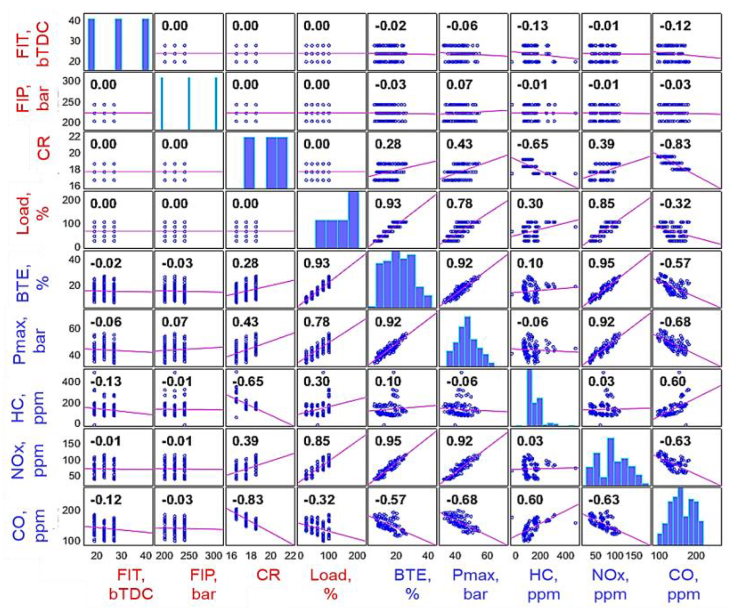
The data gathered from the experimental work was collected at different control factors, namely, the compression ratio, pilot injection timing, and pressure. Before creating a machine learning model, correlation values and a correlation matrix were prepared and analysed. It can give useful insights and advantages in the following ways. The correlation analysis is useful for identifying correlations between variables in your dataset. Correlation coefficients may be used to identify how strongly variables are connected to one another, whether the relationship is positive or negative, and the magnitude of the association. This data can assist you in understanding the interdependence and interdependencies between variables. The correlation analysis aids in the detection of multicollinearity, defined as a strong correlation amongst predictor variables. Multicollinearity can have a severe influence on machine learning model performance and interpretability, resulting in unstable coefficients and exaggerated standard errors. One may handle multicollinearity concerns by finding variables with strong correlations and deleting duplicate variables [45,46]. The correlation analysis for the data used in the present study is listed in

Table 3. Correlation values.

	FIT (bTDC)	FIP (bar)	CR	Load (%)	BTE (%)	Pmax (bar)	HC (ppm)	NOx (ppm)	CO (ppm)
FIT (bTDC)	1
FIP (bar)	0	1
CR	0	0	1
Load (%)	0	0	0	1
BTE (%)	−0.0206	−0.0258	0.2760	0.9328	1
Pmax (bar)	−0.0637	0.0691	0.4257	0.7758	0.9204	1
HC (ppm)	−0.1328	−0.0066	−0.6458	0.2995	0.1001	−0.0594	1
NOx (ppm)	−0.0131	−0.0109	0.3921	0.8521	0.9456	0.9215	0.0298	1
CO (ppm)	−0.1153	−0.0287	−0.8259	−0.3192	−0.5716	−0.6756	0.5998	−0.6270	1

.

The pairwise correlation coefficients between variables are represented by the correlation matrix. It expresses the strength and direction of a linear relationship between two variables numerically. BTE (%) has a 0.277 positive association with CR (compression ratio) and a 0.933 strong positive correlation with Load (%). This implies that BTE (%) rises with increasing compression ratios and engine load. Pmax (bar) shows a 0.426 moderate positive correlation with CR and a 0.776 strong positive connection with Load (%). This implies that as compression ratios and engine load rise, so does Pmax (bar). HC (ppm) has a high negative association with CR of −0.646, implying that as the compression ratio increases, so do the HC emissions. NOx (ppm) has a 0.392 positive association with CR and a 0.852 strong positive correlation with Load (%). This suggests that NOx emissions rise with greater compression ratios and engine load. CO (ppm) has a high negative association with CR of −0.826, implying that as the compression ratio increases, so do CO emissions. Overall, the correlation matrix sheds light on the links that exist between the variables in the dataset. It aids in understanding how changes in one variable may be related to changes in other variables, which may be useful for further research and model building. NOx (ppm) has a 0.392 positive association with CR and a 0.852 strong positive correlation with Load (%). This suggests that NOx emissions rise with greater compression ratios and engine load. CO (ppm) has a high negative association with CR of −0.826, implying that as the compression ratio increases, so do CO emissions. Overall, the correlation matrix sheds light on the links that exist between the variables in the dataset. It aids in understanding how changes in one variable may be related to changes in other variables, which may be useful for further research and model building [47,48]. The Figure 2 depicts the pair wise correlation matrix of the data used in the present study.

3.2. BTE Model

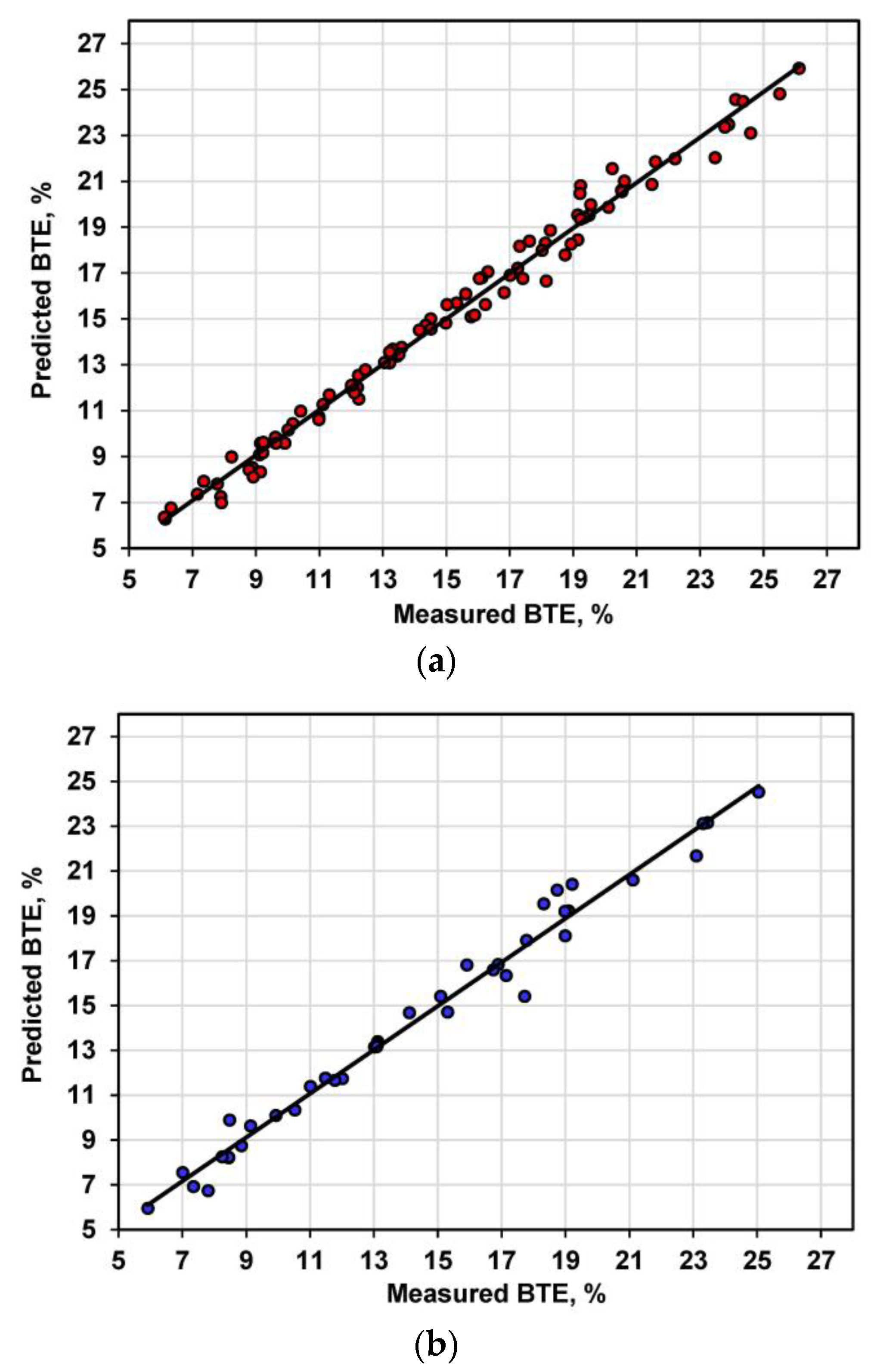
Using the XGBoost machine learning approach, the data gathered from experimental testing was used to construct a prediction model for brake thermal efficiency (BTE). The model’s goal was to forecast the BTE of a biogas–diesel dual fuel engine based on the engine loads, compression ratio, and injection parameters (pressures and timing), while using the peak pressure, nitrogen oxides (NOx), carbon monoxide (CO), and unburned hydrocarbons as the response variables. The use of the increased compression ratio helped in improvement of BTE with a peak BTE at 26.12% that could be achieved at an 18.5 compression ratio 220 bar fuel injection pressure peak engine load. Several statistical indicators were used to assess the performance of the model for prediction. With a high coefficient of determination (R²) value of 0.9865 during the training phase, the model was able to account for 98.65% of the variation in BTE. The correlation coefficient (R) of 0.9933 indicates that the anticipated and actual BTE values have a strong positive linear connection. The mean squared error (MSE) is 0.3711, while the mean absolute error (MAE) is 0.4499. The model performance depicting a comparative analysis of measured and predicted BTE values during the model training phase is illustrated in Figure 3a. Additionally, the comparative analysis of actual and model-predicted values during the model test phase is depicted in Figure 3b. It can be observed that most of the comparative points lie close to the 45° line (best fit), showing a robust model performance [27]. It can also be observed that the model performance improved during the model test phase. The model’s statistical evaluation is listed in

Table 4. Statistical evaluation of models.

Phase	Parameter	R2	R	MSE	MAE
Training	BTE	0.9865	0.9933	0.3711	0.4499
	Pmax	0.9626	0.9811	1.4236	0.9665
	HC	0.9494	0.9744	125.8	8.4312
	NOx	0.9722	0.986	12.8302	3.089
	CO	0.9576	0.9786	24.72	4.23
Test	BTE	0.9890	0.9945	0.2845	0.4412
	Pmax	0.9777	0.9888	1.14	0.932
	HC	0.9628	0.9812	101.7	5.89
	NOx	0.9797	0.9898	8.45	2.014
	CO	0.9645	0.9821	17.36	3.15

.

Similarly, the model’s performance was assessed using a second test dataset. The test phase yielded good findings, with an R² value of 0.9890, suggesting that the model can explain 98.90% of the variation in BTE. The correlation coefficient (R) of 0.9945 indicates that the anticipated and actual BTE values in the test dataset have a strong positive linear connection. The model’s accuracy in predicting BTE is further illustrated by the lower MSE value of 0.2845 and the MAE value of 0.4412.

These assessment measures demonstrate the potency and dependability of the created prediction model for calculating BTE in the dual-fuel biogas-diesel engine. The model can provide accurate predictions and can be a useful tool for enhancing engine performance and emissions, according to the high R² values, significant correlations, and low error values.

3.3. Pmax Model

Using the XGBoost machine learning approach, the experimental data acquired from the biogas–diesel-powered dual-fuel engine has been used to construct a peak pressure prediction model. Based on the injection parameters (pressures and timing), compression ratio, and engine loads, the model attempted to forecast the peak pressure. Several statistical measures were used to assess model performance, including R² (coefficient of determination), R (correlation coefficient), MSE (mean squared error), and MAE (mean absolute error). These metrics give information about the prediction model’s accuracy and dependability. During the training phase, the model attained an R² value of 0.9626, suggesting that the model can explain 96.26% of the variation in peak pressure. The R-value of 0.9811 indicates a significant positive association. The R-value of 0.9811 indicates that the anticipated and actual peak pressure levels are well correlated. The MSE value of 1.4236 reflects the average squared difference between predicted and actual values, whilst the MAE value of 0.9665 shows the average absolute difference. Figure 4a depicts the model performance during the model training phase, which includes a comparison of measured and anticipated Pmax values. Figure 4b also shows the comparative analysis of actual and model projected values throughout the model test phase. It can be seen that the majority of the compared points are near the 45° line (best fit), indicating a strong model performance [25,49]. It is also worth noting that model performance increased during the model testing phase. The model’s statistical evaluation is given in Table 4.

During the testing phase, the model performed even better. It obtained an R² value of 0.9777, suggesting that the model can explain 97.77% of the variance in peak pressure. The R-value of 0.9888 indicates that the anticipated and actual values are strongly correlated. When compared to the training phase, the MSE value of 1.14 shows a reduced average squared difference between predicted and actual values. A smaller average absolute difference is represented by the MAE value of 0.932. These findings show that the prediction model constructed using the XGBoost ML approach predicts the peak pressure of the biogas–diesel driven dual fuel engine well. The model’s correctness and dependability in capturing the link between the input parameters and the response variable are demonstrated by the high R² and R values, as well as the low MSE and MAE values.

3.4. Unburnt Hydrocarbon Model

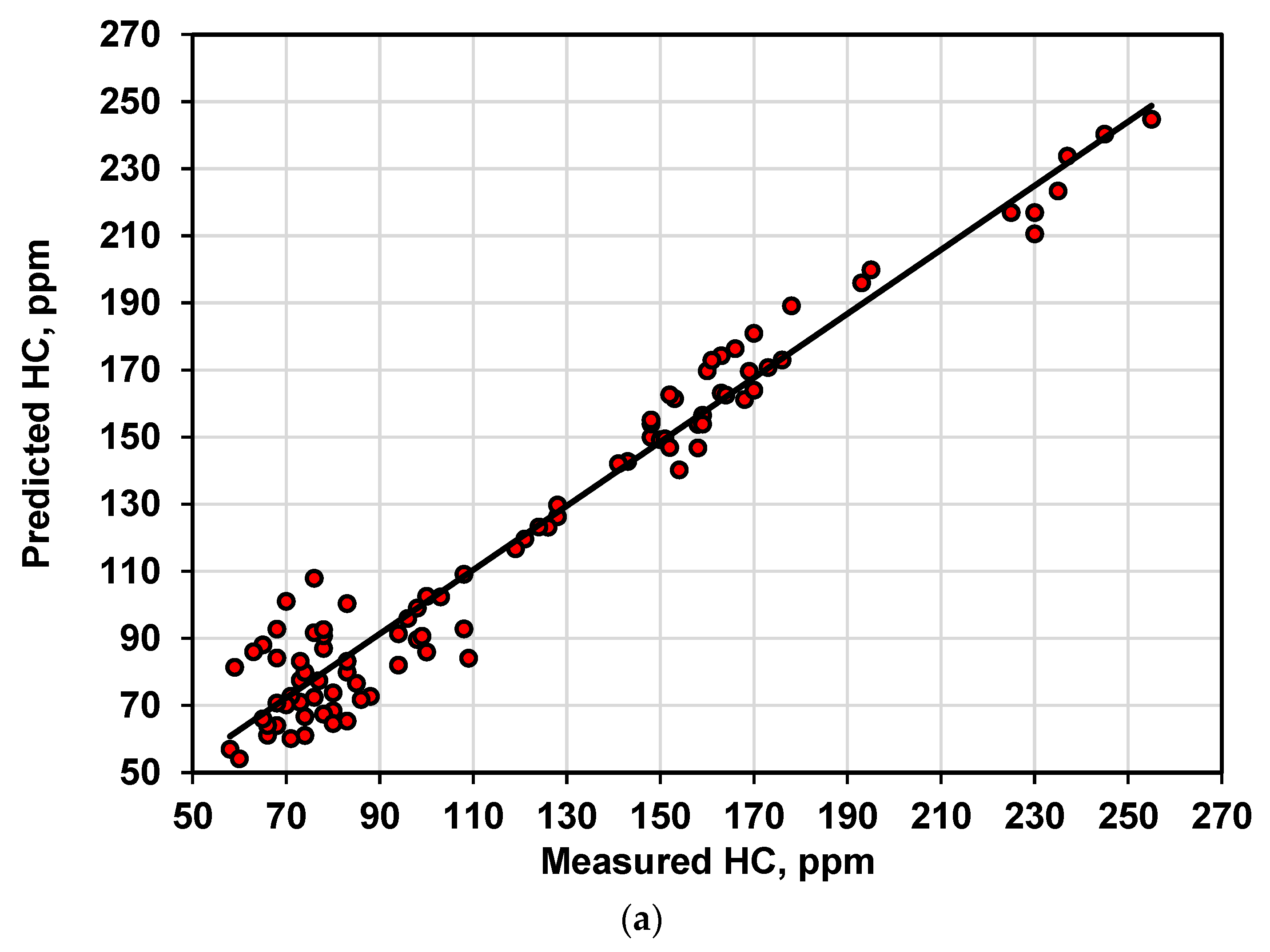
Using the XGBoost machine learning approach, the experimental data from the biogas–diesel-fueled to the dual-fuel engine was used to construct a prediction model for HC emission. Control elements included injection settings (pressures and timing), the ratio of compression, and engine loads, with HC emission serving as the response variable. To examine the performance of the constructed prediction model, numerous statistical indicators were used. During the training phase, the model attained an R-squared value of 0.9494, suggesting that it could explain 94.94% of the variation in HC emissions. The correlation coefficient (R) was 0.9744, indicating a significant positive linear association between anticipated and actual HC values. The training phase’s mean squared error (MSE) was estimated to be 125.8, representing the average squared difference between predicted and real HC values. The average absolute difference (MAD) between anticipated and actual HC values was determined to be 8.4312. Figure 5a demonstrates model performance throughout the training period, including a comparison of measured and predicted HC emission values. Throughout the model testing process, Figure 5b shows a comparative analysis of actual and model projected values. The majority of the comparison points are near the 45° line (best fit), suggesting a good model performance. It should also be noted that model performance improved during the model testing phase. The model’s statistical evaluation is depicted in Table 4.

A different test dataset was also used to check the model’s generalization capacity. During the testing phase, the model produced encouraging results, with an R-squared value of 0.9628, suggesting that the model could explain 96.28% of the variation in HC emissions. For the test phase, the correlation coefficient (R) was estimated to be 0.9812, showing a significant positive linear connection between the anticipated and actual HC values. The MSE of the test phase was also calculated to be 101.7, signifying the average squared difference between the predicted and real HC values in the test dataset. The MAE in the test dataset was determined to be 5.89, showing the average absolute difference between the anticipated and actual HC values. Overall, the XGBoost ML prediction model demonstrated excellent accuracy and significant predictive skills for forecasting HC emissions in the biogas–diesel-driven dual-fuel engine. These findings indicate the model’s ability to capture the intricate interactions between control parameters and HC emissions, offering useful insights for engine optimization and emission control measures.

3.5. NOx Model

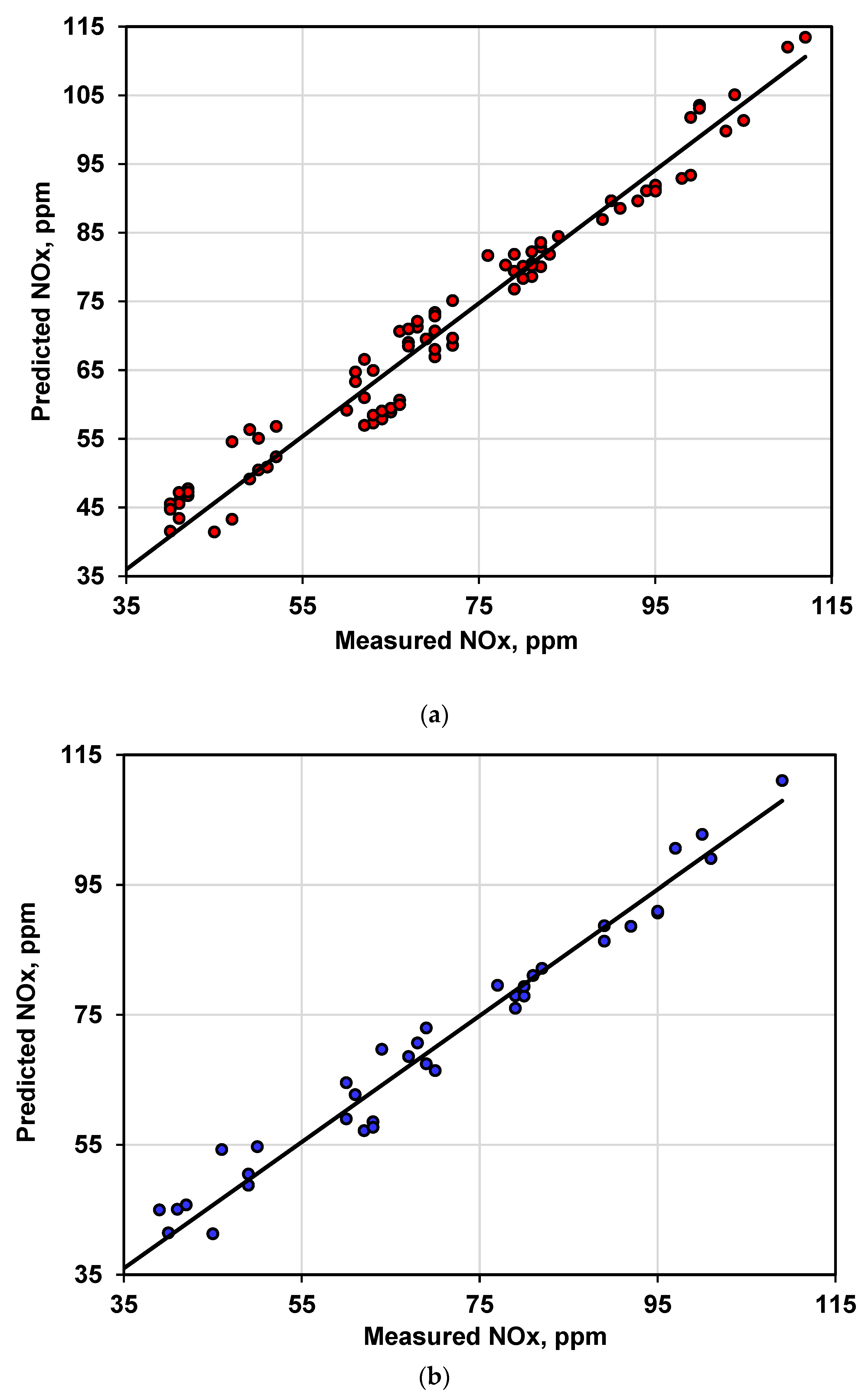
The experimental data was utilized to create a prediction model for NOx emissions in a biogas–diesel-driven dual-fuel engine. The model was built with the XGBoost machine learning approach, and control elements included injection settings (pressures and timing), compression ratio, and engine loads. The response variable was chosen to be NOx emission. Several statistical indicators were used to assess the prediction model’s performance. The model achieved a high coefficient of determination (R²) value of 0.9722 during the training phase, suggesting that it can explain around 97.22% of the variation in NOx emissions. The correlation coefficient (R) was 0.986, showing a significant positive link between expected and actual NOx levels. MSE stands for the mean squared error. The mean squared error (MSE) was calculated to be 12.8302, which is the average squared difference between the anticipated and actual NOx levels. The mean absolute error (MAE) in the training period was estimated to be 3.089, signifying the average absolute difference between the predicted and real NOx levels. On the test dataset, the model’s performance was subsequently evaluated. The test phase R² score was 0.9797, suggesting that the model could clarify about 97.97% of the variation in NOx emissions for unknown data. The correlation coefficient (R) was calculated to be 0.9898, showing a high positive link between projected and actual NOx levels throughout the test phase. The mean squared error (MSE) was 8.45, representing the average squared difference between the expected and actual results. Figure 6a depicts the model performance throughout the course of the training period, including a comparison of measured and anticipated NOx emission levels. Figure 6b depicts a comparison of actual and model-predicted values throughout the model testing procedure. The majority of the comparison points are close to the 45° line (best fit), indicating that the model performed well. It should also be mentioned that during the model testing phase, the model performance increased. The model’s statistical evaluation is shown in Table 4.

The mean squared error (MSE) for the test dataset was 8.45, showing the average squared difference between anticipated and actual NOx levels. The mean absolute error (MAE) in the test phase was estimated to be 2.014, signifying the average absolute difference between the expected and actual NOx values. These assessment metrics reveal that the created prediction model employing the XGBoost ML approach predicts NOx emissions for the biogas–diesel-fueled dual fuel engine with a good level of accuracy and dependability. The model performs well on both the training and test datasets, indicating that it has the potential to be useful in predicting NOx emissions based on the input parameters.

3.6. CO Model

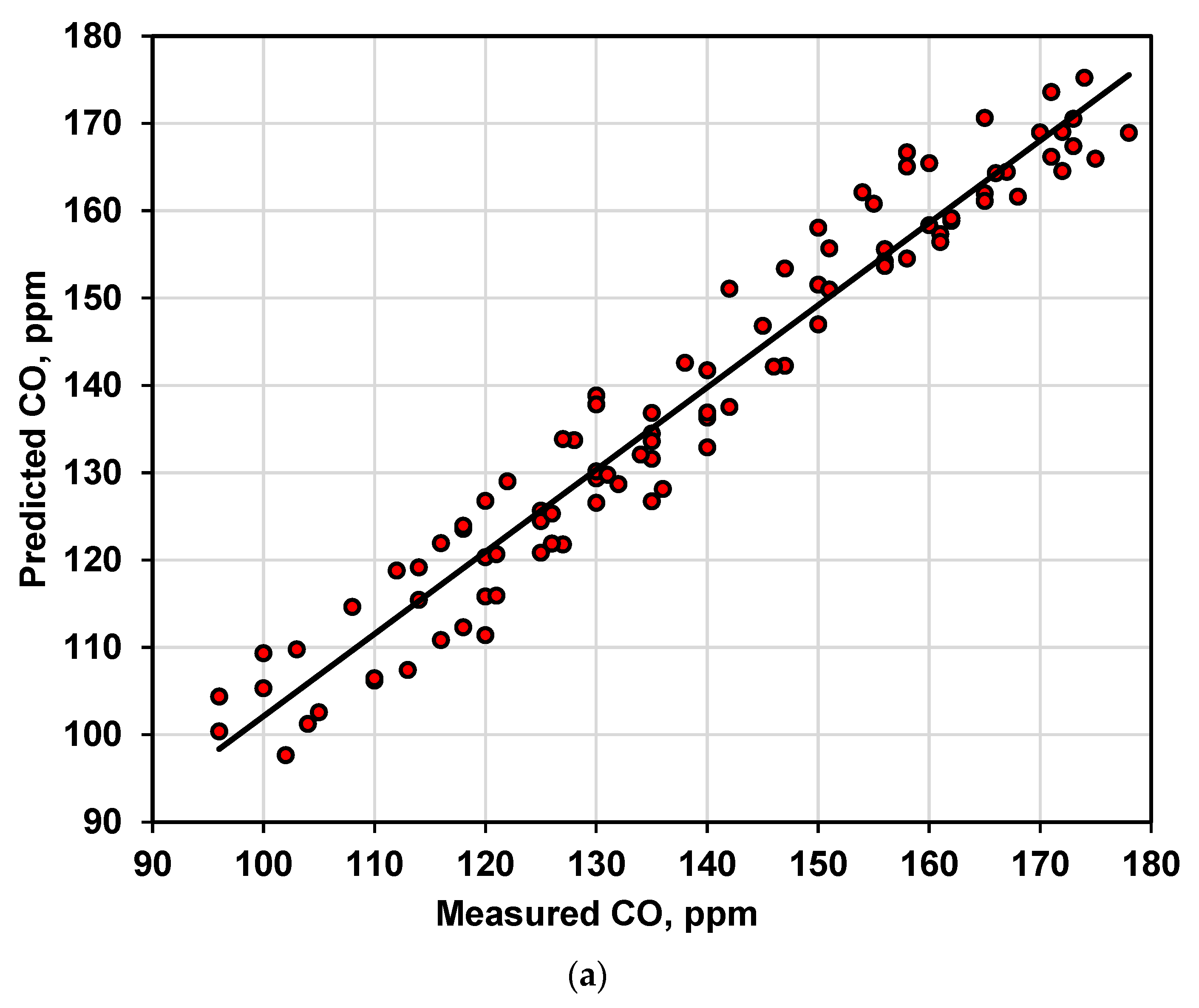
The prediction model created for a biogas–diesel-powered dual fuel engine utilizing the XGBoost machine learning approach focused on modelling CO emissions based on different injection parameters (pressures and timing), the ratio of compression, and engine loads. The data from the experiments were used to train and test the model. The prediction model’s performance was evaluated using several measures. The coefficient of determination (R²) was determined to determine the fraction of the variance in CO emissions that the model could explain. The model attained an R² value of 0.9576 during the training phase, showing a significant connection between projected and actual CO emissions. Figure 7a depicts model performance over the course of the training period, including a comparison of measured and estimated CO emission levels. Figure 7b depicts a comparison of actual and model-predicted values throughout the model-testing procedure. The majority of the comparison points are close to the 45° line (best fit), indicating that the model performed well. It should also be mentioned that during the model testing phase, model performance increased. The model’s statistical evaluation is shown in Table 4.

The correlation coefficient (R) was utilized as well to assess the strength and direction of the linear relationship. To assess the intensity and direction of the linear relationship between expected and actual CO emissions, the correlation coefficient (R) was calculated. The model acquired an R-value of 0.9786 during the training phase, showing a significant positive correlation. To measure the accuracy of the model’s predictions, the mean squared error (MSE) and mean absolute error (MAE) were determined. The MSE is the average squared difference between the expected and actual CO emission levels, whereas the MAE is the average absolute difference. The model attained an MSE of 24.72 and an MAE of 4.23 during the training phase, showing reasonably low prediction errors. The model’s generalization ability was also evaluated on previously encountered data. During the testing phase, the model performed consistently, with an R² value of 0.9645 and an R-value of 0.9821. In the test phase, the MSE and MAE were 17.36 and 3.15, confirming the model’s capacity to generate accurate predictions on fresh data.

Overall, the prediction model performed well in projecting CO emissions for the biogas–diesel dual-fuel engine. The strong R² and R values, as well as the low MSE and MAE, indicate that the model is successful at capturing the correlations between injection parameters, the compression ratio, engine loads, and CO emissions.

4. Conclusions

The current study investigates the feasibility of using waste-derived biogas as an alternative fuel for dual-fuel engines that use diesel as a pilot fuel. A strong machine learning algorithm called XGBoost was used to precisely analyse engine performance. Extensive laboratory-based data was gathered through testing in order to construct prognosis models for each output variable of relevance. Critical engine control elements such as pilot fuel injection pressure, engine load, and pilot fuel injection time are all taken into account in the models. This comprehensive approach yielded several valuable insights into optimizing engine performance by modelling the influence of these control elements on various engine response variables such as brake thermal efficiency, brake-specific fuel consumption, oxides of nitrogen, carbon monoxide, and unburnt hydrocarbons. The following are the main outcomes of the investigation:

• The results show the models’ durability and correctness, with R² values that range from 0.9628 to 0.9892 and Pearson’s coefficients ranging from 0.9812 to 0.9945.
• The models also had low mean absolute error values that ranged from 0.4412 to 5.89, as well as mean squared error values ranging from 0.2845 to 101.7.
• The comparison of measured and predicted values reveals a good prognostic model as most of the data points are on the best fit line.
• The higher compression ratio (18.5) helped in improving the problem of low brake thermal efficiency.
• The lower combustion temperature owing to low energy density helped in the reduction of NOx emission.
• These results demonstrate the accuracy with which test prognostic models capture the intricate links between control settings and engine performance metrics.

Furthermore, this study helps to enhance dual-fuel engine technology by using waste-derived biogas as a sustainable fuel source. The findings have ramifications for the transportation industry, as the use of such engines has the potential to reduce emissions and environmental impacts. This paves the path for more sustainable and environmentally friendly transportation solutions by utilizing waste materials for energy generation. Overall, this research marks a substantial advancement in the performance and environmental sustainability of dual-fuel engines that use waste-derived biogas.

References

1. Thirunavukkarasu, M.; Sawle, Y.; Lala, H. A Comprehensive Review on Optimization of Hybrid Renewable Energy Systems Using Various Optimization Techniques. Renew. Sustain. Energy Rev. 2023, 176, 113192. [Google Scholar] [CrossRef]
2. Thanigaivel, S.; Vickram, S.; Dey, N.; Gulothungan, G.; Subbaiya, R.; Govarthanan, M.; Karmegam, N.; Kim, W. The Urge of Algal Biomass-Based Fuels for Environmental Sustainability against a Steady Tide of Biofuel Conflict Analysis: Is Third-Generation Algal Biorefinery a Boon? Fuel 2022, 317, 123494. [Google Scholar] [CrossRef]
3. Woertz, I.C.; Benemann, J.R.; Du, N.; Unnasch, S.; Mendola, D.; Mitchell, B.G.; Lundquist, T.J. Life Cycle GHG Emissions from Microalgal Biodiesel—A CA-GREET Model. Environ. Sci. Technol. 2014, 48, 6060–6068. [Google Scholar] [CrossRef] [PubMed]
4. Liu, Y.; Gao, C.; Lu, Y. The Impact of Urbanization on GHG Emissions in China: The Role of Population Density. J. Clean. Prod. 2017, 157, 299–309. [Google Scholar] [CrossRef]
5. Wang, S.; Zhang, Z.; Hou, X.; Lv, J.; Lan, G.; Yang, G.; Hu, J. The Environmental Potential of Hydrogen Addition as Complementation for Diesel and Biodiesel: A Comprehensive Review and Perspectives. Fuel 2023, 342, 127794. [Google Scholar] [CrossRef]
6. Das, S.; Kashyap, D.; Kalita, P.; Kulkarni, V.; Itaya, Y. Clean Gaseous Fuel Application in Diesel Engine: A Sustainable Option for Rural Electrification in India. Renew. Sustain. Energy Rev. 2020, 117, 109485. [Google Scholar] [CrossRef]
7. Kim, M.K.; Park, D.; Kim, M.; Heo, J.; Park, S.; Chong, H. Article the Characteristics and Distribution of Chemical Components in Particulate Matter Emissions from Diesel Locomotives. Atmosphere 2021, 12, 70. [Google Scholar] [CrossRef]
8. Verma, P.; Stevanovic, S.; Zare, A.; Dwivedi, G.; Van, T.C.; Davidson, M.; Rainey, T.; Brown, R.J.; Ristovski, Z.D. An Overview of the Influence of Biodiesel, Alcohols, and Various Oxygenated Additives on the Particulate Matter Emissions from Diesel Engines. Energies 2019, 12, 1987. [Google Scholar] [CrossRef] [Green Version]
9. Singh, P.; Kumar, R.; Sharma, S.; Kumar, S. Effect of Engine Parameters on the Performance of Dual-Fuel CI Engines with Producer Gas—A Review. Energy Fuels 2021, 35, 16377–16402. [Google Scholar] [CrossRef]
10. Fiore, M.; Magi, V.; Viggiano, A. Internal Combustion Engines Powered by Syngas: A Review. Appl. Energy 2020, 276, 115415. [Google Scholar] [CrossRef]
11. Said, Z.; Sharma, P.; Thi Bich Nhuong, Q.; Bora, B.J.; Lichtfouse, E.; Khalid, H.M.; Luque, R.; Nguyen, X.P.; Hoang, A.T. Intelligent Approaches for Sustainable Management and Valorisation of Food Waste. Bioresour. Technol. 2023, 377, 128952. [Google Scholar] [CrossRef]
12. Patra, B.R.; Nanda, S.; Dalai, A.K.; Meda, V. Slow Pyrolysis of Agro-Food Wastes and Physicochemical Characterization of Biofuel Products. Chemosphere 2021, 285, 131431. [Google Scholar] [CrossRef]
13. Kumar, S.; Dinesha, P. Optimization of Engine Parameters in a Bio Diesel Engine Run with Honge Methyl Ester Using Response Surface Methodology. Measurement 2018, 125, 224–231. [Google Scholar] [CrossRef]
14. Toledo-Cervantes, A.; Serejo, M.L.; Blanco, S.; Pérez, R.; Lebrero, R.; Muñoz, R. Photosynthetic Biogas Upgrading to Bio-Methane: Boosting Nutrient Recovery via Biomass Productivity Control. Algal Res. 2016, 17, 46–52. [Google Scholar] [CrossRef] [Green Version]
15. Bose, A.; O’Shea, R.; Lin, R.; Long, A.; Rajendran, K.; Wall, D.; De, S.; Murphy, J.D. Evaluation of a Biomethane, Food and Biofertiliser Polygeneration System in a Circular Economy System. Renew. Sustain. Energy Rev. 2022, 170, 112960. [Google Scholar] [CrossRef]
16. Khan, M.U.; Lee, J.T.E.; Bashir, M.A.; Dissanayake, P.D.; Ok, Y.S.; Tong, Y.W.; Shariati, M.A.; Wu, S.; Ahring, B.K. Current Status of Biogas Upgrading for Direct Biomethane Use: A Review. Renew. Sustain. Energy Rev. 2021, 149, 111343. [Google Scholar] [CrossRef]
17. Ardolino, F.; Cardamone, G.F.; Parrillo, F.; Arena, U. Biogas-to-Biomethane Upgrading: A Comparative Review and Assessment in a Life Cycle Perspective. Renew. Sustain. Energy Rev. 2021, 139, 110588. [Google Scholar] [CrossRef]
18. Prabhu, A.V.; Avinash, A.; Brindhadevi, K.; Pugazhendhi, A. Performance and Emission Evaluation of Dual Fuel CI Engine Using Preheated Biogas-Air Mixture. Sci. Total Environ. 2021, 754, 142389. [Google Scholar] [CrossRef]
19. Khayum, N.; Anbarasu, S.; Murugan, S. Combined Effect of Fuel Injecting Timing and Nozzle Opening Pressure of a Biogas-Biodiesel Fuelled Diesel Engine. Fuel 2020, 262, 116505. [Google Scholar] [CrossRef]
20. Verma, S.; Das, L.M.; Kaushik, S.C.; Tyagi, S.K. An Experimental Investigation of Exergetic Performance and Emission Characteristics of Hydrogen Supplemented Biogas-Diesel Dual Fuel Engine. Int. J. Hydrog. Energy 2018, 2018, 2452–2468. [Google Scholar] [CrossRef]
21. Das, S.; Kashyap, D.; Bora, B.J.; Kalita, P.; Kulkarni, V. Thermo-Economic Optimization of a Biogas-Diesel Dual Fuel Engine as Remote Power Generating Unit Using Response Surface Methodology. Therm. Sci. Eng. Prog. 2021, 24, 100935. [Google Scholar] [CrossRef]
22. Benaissa, S.; Adouane, B.; Ali, S.M.; Rashwan, S.S.; Aouachria, Z. Investigation on Combustion Characteristics and Emissions of Biogas/Hydrogen Blends in Gas Turbine Combustors. Therm. Sci. Eng. Prog. 2022, 27, 101178. [Google Scholar] [CrossRef]
23. Salam, S.; Choudhary, T.; Pugazhendhi, A.; Verma, T.N.; Sharma, A. A Review on Recent Progress in Computational and Empirical Studies of Compression Ignition Internal Combustion Engine. Fuel 2020, 279, 118469. [Google Scholar] [CrossRef]
24. Sharma, P.; Said, Z.; Kumar, A.; Nižetić, S.; Pandey, A.; Hoang, A.T.; Huang, Z.; Afzal, A.; Li, C.; Le, A.T.; et al. Recent Advances in Machine Learning Research for Nanofluid-Based Heat Transfer in Renewable Energy System. Energy Fuels 2022, 36, 6626–6658. [Google Scholar] [CrossRef]
25. Karunamurthy, K.; Janvekar, A.A.; Palaniappan, P.L.; Adhitya, V.; Lokeswar, T.T.K.; Harish, J. Prediction of IC Engine Performance and Emission Parameters Using Machine Learning: A Review. J. Therm. Anal. Calorim. 2023, 148, 3155–3177. [Google Scholar] [CrossRef]
26. Aliramezani, M.; Koch, C.R.; Shahbakhti, M. Modeling, Diagnostics, Optimization, and Control of Internal Combustion Engines via Modern Machine Learning Techniques: A Review and Future Directions. Prog. Energy Combust. Sci. 2022, 88, 100967. [Google Scholar] [CrossRef]
27. Sahoo, S.; Kumar, V.N.S.P.; Srivastava, D.K. Quantitative Analysis of Engine Parameters of a Variable Compression Ratio CNG Engine Using Machine Learning. Fuel 2022, 311, 122587. [Google Scholar] [CrossRef]
28. Wang, H.; Ji, C.; Su, T.; Shi, C.; Ge, Y.; Yang, J.; Wang, S. Comparison and Implementation of Machine Learning Models for Predicting the Combustion Phases of Hydrogen-Enriched Wankel Rotary Engines. Fuel 2022, 310, 122371. [Google Scholar] [CrossRef]
29. Bora, B.J.; Dai Tran, T.; Prasad Shadangi, K.; Sharma, P.; Said, Z.; Kalita, P.; Buradi, A.; Nhanh Nguyen, V.; Niyas, H.; Tuan Pham, M.; et al. Improving Combustion and Emission Characteristics of a Biogas/Biodiesel-Powered Dual-Fuel Diesel Engine through Trade-off Analysis of Operation Parameters Using Response Surface Methodology. Sustain. Energy Technol. Assess. 2022, 53, 102455. [Google Scholar] [CrossRef]
30. Sagi, O.; Rokach, L. Approximating XGBoost with an Interpretable Decision Tree. Inf. Sci. 2021, 572, 522–542. [Google Scholar] [CrossRef]
31. Zhu, X.; Chu, J.; Wang, K.; Wu, S.; Yan, W.; Chiam, K. Prediction of Rockhead Using a Hybrid N-XGBoost Machine Learning Framework. J. Rock Mech. Geotech. Eng. 2021, 13, 1231–1245. [Google Scholar] [CrossRef]
32. Said, Z.; Sharma, P.; Bora, B.J.; Pandey, A.K. Sonication Impact on Thermal Conductivity of F-MWCNT Nanofluids Using XGBoost and Gaussian Process Regression. J. Taiwan Inst. Chem. Eng. 2023, 145, 104818. [Google Scholar] [CrossRef]
33. Yun, K.K.; Yoon, S.W.; Won, D. Prediction of Stock Price Direction Using a Hybrid GA-XGBoost Algorithm with a Three-Stage Feature Engineering Process. Expert Syst. Appl. 2021, 186, 115716. [Google Scholar] [CrossRef]
34. Zhang, M.; Chen, W.; Yin, J.; Feng, T. Lithium Battery Health Factor Extraction Based on Improved Douglas–Peucker Algorithm and SOH Prediction Based on XGboost. Energies 2022, 15, 5981. [Google Scholar] [CrossRef]
35. Ibrahem Ahmed Osman, A.; Najah Ahmed, A.; Chow, M.F.; Feng Huang, Y.; El-Shafie, A. Extreme Gradient Boosting (Xgboost) Model to Predict the Groundwater Levels in Selangor Malaysia. Ain Shams Eng. J. 2021, 12, 1545–1556. [Google Scholar] [CrossRef]
36. Qiu, Y.; Zhou, J.; Khandelwal, M.; Yang, H.; Yang, P.; Li, C. Performance Evaluation of Hybrid WOA-XGBoost, GWO-XGBoost and BO-XGBoost Models to Predict Blast-Induced Ground Vibration. Eng. Comput. 2022, 38, 4145–4162. [Google Scholar] [CrossRef]
37. Ben Jabeur, S.; Mefteh-Wali, S.; Viviani, J.L. Forecasting Gold Price with the XGBoost Algorithm and SHAP Interaction Values. Ann. Oper. Res. 2021, 1–21. [Google Scholar] [CrossRef]
38. Wang, S.; Liu, S.; Zhang, J.; Che, X.; Yuan, Y.; Wang, Z.; Kong, D. A New Method of Diesel Fuel Brands Identification: SMOTE Oversampling Combined with XGBoost Ensemble Learning. Fuel 2020, 282, 118848. [Google Scholar] [CrossRef]
39. Pan, S.; Zheng, Z.; Guo, Z.; Luo, H. An Optimized XGBoost Method for Predicting Reservoir Porosity Using Petrophysical Logs. J. Pet. Sci. Eng. 2022, 208, 109520. [Google Scholar] [CrossRef]
40. Thongsuwan, S.; Jaiyen, S.; Padcharoen, A.; Agarwal, P. ConvXGB: A New Deep Learning Model for Classification Problems Based on CNN and XGBoost. Nucl. Eng. Technol. 2021, 53, 522–531. [Google Scholar] [CrossRef]
41. Li, X.; Ma, L.; Chen, P.; Xu, H.; Xing, Q.; Yan, J.; Lu, S.; Fan, H.; Yang, L.; Cheng, Y. Probabilistic Solar Irradiance Forecasting Based on XGBoost. Energy Rep. 2022, 8, 1087–1095. [Google Scholar] [CrossRef]
42. Zhang, P.; Jia, Y.; Shang, Y. Research and Application of XGBoost in Imbalanced Data. Int. J. Distrib. Sens. Netw. 2022, 18, 15501329221106935. [Google Scholar] [CrossRef]
43. Roy, S.; Ghosh, A.; Das, A.K.; Banerjee, R. Development and Validation of a GEP Model to Predict the Performance and Exhaust Emission Parameters of a CRDI Assisted Single Cylinder Diesel Engine Coupled with EGR. Appl. Energy 2015, 140, 52–64. [Google Scholar] [CrossRef]
44. Sharma, P.; Said, Z.; Memon, S.; Elavarasan, R.M.; Khalid, M.; Nguyen, X.P.; Arıcı, M.; Hoang, A.T.; Nguyen, L.H. Comparative Evaluation of AI-Based Intelligent GEP and ANFIS Models in Prediction of Thermophysical Properties of Fe3O4-Coated MWCNT Hybrid Nanofluids for Potential Application in Energy Systems. Int. J. Energy Res. 2022, 46, 19242–19257. [Google Scholar] [CrossRef]
45. Dodo, U.A.; Ashigwuike, E.C.; Abba, S.I. Machine Learning Models for Biomass Energy Content Prediction: A Correlation-Based Optimal Feature Selection Approach. Bioresour. Technol. Rep. 2022, 19, 101167. [Google Scholar] [CrossRef]
46. Kwon, B.; Ejaz, F.; Hwang, L.K. Machine Learning for Heat Transfer Correlations. Int. Commun. Heat Mass Transf. 2020, 116, 104694. [Google Scholar] [CrossRef]
47. Prasad, T.R.; Krishna, K.R.; Sharma, K.V.; Bhaskar, C.N. Correlations to Estimate Electrical Conductivity, Thermal Conductivity and Viscosity of Cobalt Nanofluid. Heat Mass Transf. 2023, 59, 95–112. [Google Scholar] [CrossRef]
48. Jebli, I.; Belouadha, F.-Z.; Kabbaj, M.I.; Tilioua, A. Prediction of Solar Energy Guided by Pearson Correlation Using Machine Learning. Energy 2021, 224, 120109. [Google Scholar] [CrossRef]
49. Liu, J.; Huang, Q.; Ulishney, C.; Dumitrescu, C.E. Machine Learning Assisted Prediction of Exhaust Gas Temperature of a Heavy-Duty Natural Gas Spark Ignition Engine. Appl. Energy 2021, 300, 117413. [Google Scholar] [CrossRef]
Figure 1. Experimental setup.
Fermentation 09 00598 g001
Figure 2. Correlation matrix of data column.
Fermentation 09 00598 g002
Figure 3. BTE model: (a) Measured vs. predicted values during model training. (b) Measured vs. predicted values during the model test.
Fermentation 09 00598 g003
Figure 4. Pmax model: (a) Measured vs. predicted values during model training. (b) Measured vs. predicted values during model test.
Fermentation 09 00598 g004
Figure 5. HC model: (a) Measured vs. predicted values during model training. (b) Measured vs. predicted values during model test.
Fermentation 09 00598 g005aFermentation 09 00598 g005b
Figure 6. NOx model: (a) Measured vs. predicted values during model training. (b) Measured vs. predicted values during the model test.
Fermentation 09 00598 g006
Figure 7. CO model: (a) Measured vs. predicted values during model training. (b) Measured vs. predicted values during model test.
Fermentation 09 00598 g007aFermentation 09 00598 g007b