Stern Duct with NACA Foil Section Designed by Resistance and Self-Propulsion Simulation for Japan Bulk Carrier

Abstract

The objective of the presented work is the stern duct design for the JBC (Japan Bulk Carrier) hull form. Since the original duct only provides a 0.6% resistance reduction, an innovative duct will be proposed to improve the ship resistance and propulsion performance. The duct section geometry is based on the NACA (National Advisory Committee for Aeronautics) 4-digit foil series. First, we analyze whether the wake flow field and total resistance of the ship are improved, and then we investigate the self-propulsion performance for the selected ones. The research tool is the CFD (Computational Fluid Dynamics) software OpenFOAM 9 with the viscous free surface flow field modelled by the VOF (Volume of Fluid) method and the SST (Shear Stress Transport) k–ω turbulence model. The propeller effect is implemented by the MRF (Multi-Reference Frame). Compared to the original duct, two ducts, namely, NACA 7908 and NACA 6.3914, show the best (2.8%) resistance reduction in the bare hull condition. By installing both ducts, the propeller thrust decreases 6 and 5% to reach the self-propulsion point, and the behind-hull efficiency increases 7 and 6%. Both ducts save the energy, i.e., effective horsepower, by 4.3%, and produce obvious flow acceleration, achieving around 10% higher effective wake factor (1 − w). The nominal and propeller wakes are improved as well.

1. Introduction

Against the growing threat of global warming, extreme weather, and climate change mitigation, countries and international organizations have long and constantly paid attention to environmental issues. Progressively strict regulations have been imposed on marine transportation such as carbon emission reduction. The sea shipping industry emitted one billion tons of CO₂ globally in 2018. The Emissions Trading System (ETS) had just taken effect on the very first day of 2024, and the ships berthing in EU (European Union) ports will face the carbon tax bill reaching USD 3.6 billion. The next stage of ETS will cover 100% carbon emission. The research and development of energy saving technology is crucial to pursue low, even zero, carbon emissions as the primary goal for ship design.

Based on the installation location of the energy saving devices (ESDs), there are several types of ESD. They can be installed: (1) on the ship’s stern in front of the propeller, or (2) on the propeller, or (3) behind the propeller on the rudder or even behind the rudder, or (4) a combination of the above-mentioned methods. ESDs have been practically used on newly designed ships or refurbished old ships.

Our study objective: The JBC (Japan Bulk Carrier) ship model and its type (1) ESDs, i.e., a stern duct (pre-duct, energy saving duct) in front of the propeller, were proposed by the T2015 (Tokyo 2015 Workshop on CFD in Ship Hydrodynamics; CFD = Computational Fluid Dynamics) [1] along with the experimental data of resistance and propulsion. The original duct is axisymmetric, with the NACA (National Advisory Committee for Aeronautics) 4420 section providing only a 0.6% reduction for the calm water bare hull resistance. Therefore, the presented work aims to further improve resistance reduction and achieve a better self-propulsion performance.

The ESDs of type (1) are the main concern of this study, which commonly consist of a duct, vortex generators, spoilers, fins, stators, or their combination. The WED (Wake Equalization Duct) developed by Schneekluth Hydrodynamik GmbH [2] claimed a fuel saving of up to 12%, and 50% lower vibration. On a container ship model measurement, the inward flow angle along the ship’s longitudinal axis on the propeller plane behind the duct is reduced to 7° from 20°. Sanoyas shipbuilding Co., Ltd., Osaka, Japan [3] deployed STF (Sanoyas Tandem Fin) in front of their ACE (Advanced flow Controlling and Energy saving) duct. The fuel consumption decreased by 8%. One STF is above the shaft tube, and another one is placed more upstream around shaft axis height. The ACE is an upper half circle with a port and starboard horizontal strut. A pre-swirl stator (PSS) proposed by DSME (Daewoo Shipbuilding & Marine Engineering) was mentioned in [4], saving energy by 4$-$6%. Lee et al. [5] applied a potential theory and experiment to design axisymmetric PSS to obtain a 3% increase of propulsive efficiency. Park et al. [6] used the CFD software Star-CCM+ to design a PSS, and suggested a method to estimate the full-scale wake behind ESDs. The so-called pre-swirl duct (PSD) combined a PSS and duct, e.g., the Becker Mewis Duct^®, which lowered power output by 6.3%, based on the ship’s model test database [7]. In the earlier design, the stators were trimmed with different angles inside the duct, and later the Becker twisted fins were extended outside the duct [8]. Andersson et al. [9] proposed a PSD for a KVLCC2 (KRISO Very Large Crude Carrier 2) tanker for a full-scale CFD benchmark. Among the total of 22 CFD results collected, the power reduction was $\pm$4% on average, with a standard deviation of 1.6%.

The S-PIV (Stereoscopic Particle Image Velocimetry) measurement for the wake field behind a PSD or PSS mounted on a C259 bulk carrier was conducted by Falchi and Aloisio [10]. Three PSDs and one PSS were tested. Great insight into the fluid mechanism of the ESDs was gleaned. The objective ship was that the nominal and propeller wakes were measured on the propeller plane, and 41.4 mm behind the plane, respectively. In the nominal wakes, the fins inside the PSDs eliminated the portside bilge vortex with two vertically located vortices induced underneath the shaft tube. The flow acceleration of the propeller wake remained as the velocity distribution without ESDs. However, in the case of the PSS, the bilge vortices on the starboard and port sides only move their position. In addition, two vortices under the shaft tube and starboard outer region were generated. Corresponding to the propeller wake, the high velocity profile deforms, and another high velocity region was formed in the upper portside.

Schuiling and van Terwisga [11] reviewed the commercial duct designs chronologically, such as the MIDP (Mitsui Integrated Duct, 1981) [12], the HZN (Hitachi Zosen Nozzle, 1982) [13], the Schneekluth WED (1986) [14], the SILD (Sumitomo Integrated Lammeren Duct, 1997) [15], the IHIMU semi-circular duct (2007) [16], the Becker Mewis Duct (2009) [17], and the Kawasaki SDS-F (Semi-Duct System with contra-Fins, 2012) [18]. In their work, a BSD (Blade efficiency improving Stator Duct) [19] mounted on a chemical tanker was investigated by using the CFD code ReFRESCO for the model and full scale. The 94-m-long, 7000 DWT tanker was named STREAMLINE with a CB (block coefficient) = 0.762, and a four-bladed propeller and rudder. The turbulence model was SST (shear stress transport) k–ω, i.e., SST-2003 [20]. The double-body model was used with the sliding mesh for the propeller rotating 2 deg per time step. The total grid number N_G was 14.3 M (million) and 5.8 M for the model and full scale, respectively, with 1.8 M around the propeller. The average y+ (non-dimensional wall distance) was 0.1 and 355 on the model and full-scale ship, respectively. The power was reduced by 4.1% in the model and 3.4% at full scale. The propeller rotation rate decreased 4.1% to reach self-propulsion with a less asymmetrical propeller loading through blade circumferential positions. The propeller efficiency increased by around 6%. However, it caused 0.8% higher ship resistance because the lower pressure induced by the lift device, i.e., pre-swirl stator, led to a pressure resistance increase.

Nicorelli et al. [21] applied the CFD software StarCCM+ to study a PSD, PSS, or WED equipped on a DTC (Duisburg Test Case) hull which belonged to a typical 14000 TEU container ship. The turbulence model was realizable k–ε. The ship model was appended with a five-bladed propeller and a twisted rudder featuring a Costa bulb. RANS (Reynolds-averaged Navier–Stokes equations) simulations were performed for ship resistance and self-propulsion, and an open-water test (OPT). The sinkage and trim were predicted in RANS CFD. In addition, the OPT was also analyzed by the BEM (Boundary Element Method). The propeller was modelled by the MRF (moving reference frame) in the OPT, and by the sliding mesh for the self-propulsion. The free surface was considered by the VOF (volume of fluid) in the resistance test but neglected by the double body model in the self-propulsion test. For the model and full-scale propeller simulation, N_G = 1.2 M and 1.5 M, y+ = 15 and 60. The grid sensitivity and uncertainty analyses were conducted for ship resistance with N_G = 0.5~6.3 M, with 4% over-prediction. The reference grid was N_G = 1.3 M, the average y+ = 30 and 160 in the model and full-scale, and 2% uncertainty. For self-propulsion, the error of the wake factor (1 − w) and thrust deduction (1 − t) against the experimental value was 3~5%. To estimate self-propulsion performance for the duct and fin designs in simulation-based design optimization (SBDO), another RANS/BEM coupling method was proposed to exchange the wake data from the RANS actuator disk and to subtract propeller-induced velocity in BEM. In SBDO, 14 parameters were considered for the three fins of PSD and PSS, and four (diameter, chord, angle of attack, and maximum sectional camber) for WED. A total of 160 PSDs or PSSs, and 70 WEDs, were generated by the Uniform Latin Hypercube method. Targeting the minimal propeller delivered horsepower (DHP) with 10 evolutions for every geometry, and the optimal geometry was found among 1600 PSDs, 1600 PSSs, and 700 WEDs, individually. A 4% DHP reduction was achieved. The PSD was suggested as the most suitable device, and the full-scale RANS showed the reduction was lowered by 2.4%. The PSS performed close to the PSD or was ineffective. The WED tended to increase ship resistance.

For a Panamax bulk carrier, a stern duct and stern bluntness were designed in a study by Sakamoto et al. [22]. The duct parameter included angles of attack (AOA), chord length, and tailing edge diameter. The (1 − w) was improved by 2~3%. The hull efficiency was improved for the model and full scale by 1~3%.

Intelligent optimization algorithms have been applied in ship design, such as the MOGA (Multi-Objective Genetic Algorithm), the NSGA-II (Non-dominating Sorting Genetic Algorithm-II), and the ANN (Artificial Neural Network), etc. For instance, MOGA for a destroyer hull form [23,24] and ANN for flow control fins (FCFs) on a small container ship [25]. NSGA-II has been widely used in many aspects of ship engineering, e.g., for a destroyer hull form [26,27], a trimaran [28], FCFs on KVLCC2 [29], marine propeller [30,31], and the duct for a rim-driven thruster [32]. For the stern duct, a reduced order model-based optimization [33] and global convergence optimization [34] were proposed.

Nguyen and Chandar [33] designed the stern duct for the JBC ship model using a double body model simulation in OpenFOAM with MRF for propeller effect. The SST k–ω turbulence model was utilized. The independent grid block of duct was attached to the hull-propeller grid system by the overset method. The CFD method was verified and validated first for the self-propulsion test with 1.7 M, 3.2 M, 7.6 M grids without duct, and then a 3.2 M grid was selected for oversetting the duct. The design goal was maximum propeller propulsive efficiency ${\eta }_D$. Based on the four-digit NACA foil profile with fixed chord length, the design parameter included the thickness (0.05~0.25), camber (0~10%), AOA (0~25 deg), and ratio (0.45~0.85) between the propeller radius r and duct radius $r_D$. The reference point of $r_D$ and AOA is the duct trailing edge. The reduced order model-based optimization consisted of off- and online stages. The proper orthogonal decomposition (POD) was executed in the offline stage. In the online stage, a surrogate model using a Gaussian process regression was then built to evaluate the objective function approximately in the loop between the POD with parametric interpolation and optimizer. The optimizer was gradient-free global optimization. Consequently, ${\eta }_D$ was improved by 10%. The optimal duct was characterized by 4.5% of camber, 10.2% of thickness, 8.7 deg of AOA, and r/$r_D$ = 0.68.

Furcas et al. [34] utilized a global convergence optimization algorithm and Star-CCM+ with a k–ε turbulence model to maximize the delivered power for JBC. The error of the open water propeller simulation was less than 1% to 4% for thrust, and the torque was over-predicted by 4~8%. The resistance simulation was performed by the double body and free surface model to obtain the wave resistance for the self-propulsion simulation in the optimization process. The iterative and grid sensitivity were investigated for the double body and free surface model (N_G = 0.25 M, 0.73 M, 9.5 M), respectively. In the self-propulsion test, the body force propeller disk or sliding mesh with the realistic propeller was used. Three runs of design were performed with different parameter limits. The chord length c = 0.147~0.440D (propeller diameter), AOA: 5~35 deg, longitudinal position x = 0.016~0.75L_PP (length between particulars), and duct radius r = 0.147~0.63D. The NACA digit for camber m = 0~7, position of maximal m: p = 0~6, and thickness t = 0.15~0.25c. In run 1, the NACA4420 section remained by changing (c, AOA, x, r). In run 2, the variation of (c, AOA, x, r, m, p, t) was considered. In run 3, the duct geometric parameters were described by the B-Spline control polygon of the generator curve with (c, x, m, p) varying. The result of (c/D, r/D, AOA) of run 1 is (0.325, 0.320, 9 deg). Run 2 generated NACA 5715 with (c/D, r/D, AOA) = (0.345, 0.359, 9 deg). The product of run 3 is a non-symmetric, trapezoid-like nozzle with a longer upper base with NACA 6716 and (c/D, r/D, AOA) = (0.443, 0.404, 10.45 deg). Consequently, the delivery power was reduced by 5.9%, 6.4%, 7.2% in runs 1, 2, 3, respectively, compared to 4.9% in the original ducts. The overall propulsive efficiency was significantly improved by considering the actual ship wake profile.

In our work, the parameter of the NACA’s four digits covers the whole range for m and p, with c fixed as the original duct. AOA = 7.06 deg had been found as in our previous work [35], comparable to the 8.7 deg of [33] and 9 deg of runs 1 and 2 in [34]. t = 0.4~0.24c.

The presented work is divided into three stages to enhance the energy-saving effect of the JBC stern duct in ship resistance and self-propulsion in calm water by using CFD:

• V and V (Verification and Validation) analysis.

  a.

  Resistance simulation without the original duct;

  b.

  Resistance simulation with the original duct;

  c.

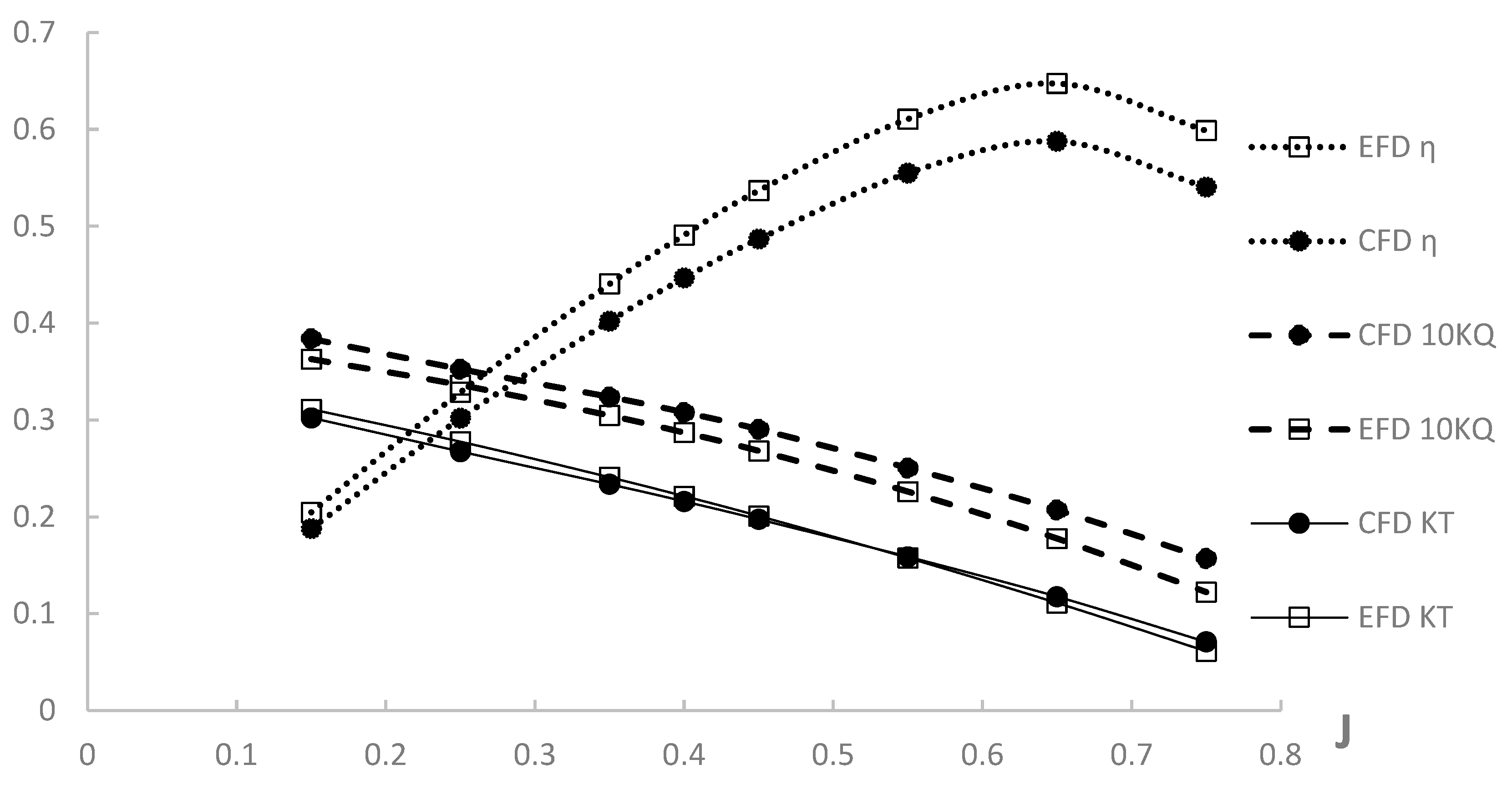
  Open-water propeller test (OPT) simulation;

  d.

  Self-propulsion simulation with the original duct.

2.

Resistance simulation with various duct designs with a NACA four-digit series foil section.

3.

Self-propulsion simulation with the optimized duct selected from the stage 2 result.

The results of stages 1,2,3 are presented in the following Section 3.1, 3.2, and 3.3, respectively. In stage 1, the V and V (Verification and Validation) analysis is conducted to ensure our CFD method is reliable before further application to the design procedure: stages 2 and 3. The V and V theory used here is based on the ITTC (International Towing Tank Conference) 75-03-01-01 guideline [36]. The simulations for V and V were conducted based on the experimental conditions of the test cases suggested by T2015 [1]. The simulation results are compared to the experimental data provided by T2015 [1], including OPT. Stages 1a, 1b, and 1d correspond to the T2015 test cases 1.1, 1.2, and 1.6, respectively. In stage 2, the lowest resistance reduction, i.e., the total ship resistance difference between the original duct and other design, is pursued. In stage 3, the self-propulsion point is simulated and found by CFD simulation for the ship with the appended optimal duct from stage 2. The improvement of self-propulsion performance compared with the original duct is discussed.

2. Methods

2.1. Numerical Schemes

The analysis and simulation tool in the presented work is the open source CFD software OpenFOAM (open-source field and manipulation) version 9 for the viscous flow simulation considering the free surface. An incompressible two-phase flow model VOF [37], i.e., interFoam solver, was applied with the SST-2003 turbulence model [20] to solve the flow field around the ship, including velocity, pressure field, and free surface elevation. The velocity and pressure coupling algorithm is PIMPLE [38], which was exclusively developed by OpenFOAM since version 2 to combine PISO (pressure implicit with splitting of operator) and SIMPLE (semi-implicit method for pressure linked equations).

The numerical schemes selected to discretize the steady Reynolds-averaged Navier–Stokes equations (RANS) and the above-mentioned flow field model are briefed as below. The temporal discretization method was the first-order Euler implicit with local time stepping. The gradient term was calculated by the first-order central difference. The second-order upwind method was used mainly for the divergence term. The Laplacian term was computed by a linear interpolation. The gradient of surface normal direction was obtained by a second-order explicit scheme with non-orthogonal corrections. The control point value of a volume or surface was also interpolated linearly. The steady propeller effect is achieved by the MRF with the realistic geometry discretization through the Coriolis term added in RANS. The ship motions, i.e., sinkage and trim, are not considered, and the ship is fixed with even keel and the uniform inflow velocity corresponding to the ship speed.

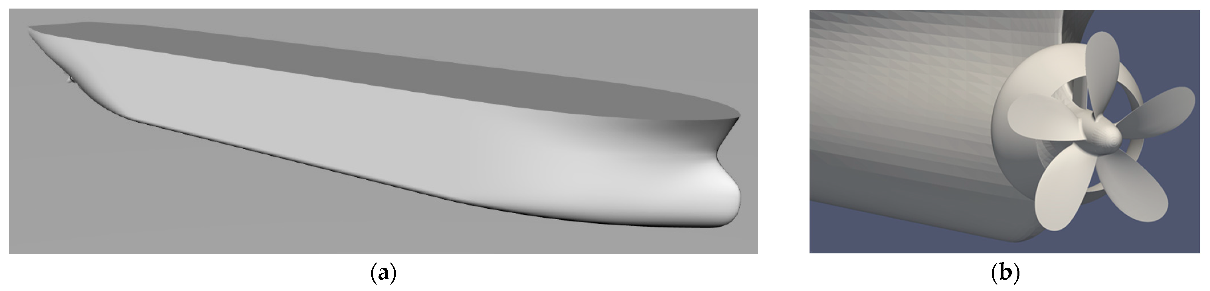
2.2. Geomtry and Test Conditions

The geometry of the JBC (Japan Bulk Carrier) ship model with and without an axisymmetric stern duct, i.e., energy saving duct, was proposed by T2015 (National Maritime Research Institute, Tokyo, Japan) [1], along with its propeller (MP. 687). The experimental data including ship resistance, self-propulsion in calm water, and open-water propeller test were provided. The ship length, beam, and draft for the 1/40 scale model are L = L_PP = 7 m (length between particulars), B_WL = 1.125 m (waterline beam), and t = 0.4125 m, respectively. The block coefficient CB = 0.8580 indicates the JBC is a full hull form. Figure 1a shows the 3D geometry of the JBC hull form generated by Rhinoceros 3D using the IGES file provided by [1]. The towing tank test condition is Froude number Fr = 0.142, corresponding to the design speed 14.5 knots in full scale and U = 1.179 m/s for the model. The Reynolds number in the model scale is Re = 7.44 $\times {10}^6$. The original duct was appended through an upward and vertical strut on the JBC stern in front of the propeller, see Figure 1b, with a 20° AOA (Angles of Attack) and a NACA 4420 section. The duct design parameters are explained at the beginning of Section 3.2.

For the 5-bladed right-rotating MP. 687 propeller, its main particulars are: diameter D = 0.203 m, pitch ratio P/D = 0.75, blade thickness ratio t/D = 0.050, hub ratio is 0.180, rake angle is 5 deg. The propeller center is at x/L_PP = 0.9854 for FP (Front Particulars) at x = 0, and z = 0.0185L_PP above the keel (baseline) or −0.0404L_PP below the waterline.

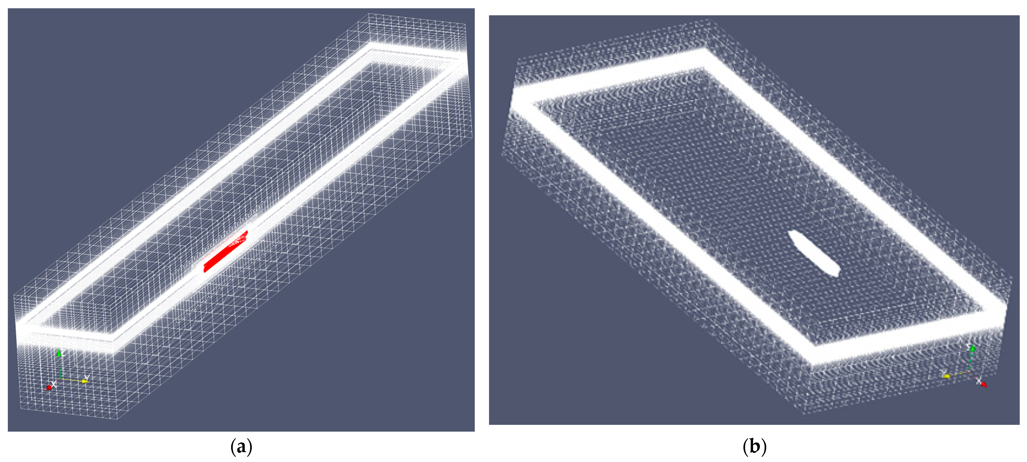
2.3. Domain and Boundary Conditions

The computational domain size is described in Figure 2, where the proper distance from the study object, i.e., the JBC hull, to the boundaries ensures the external flow fully developed and prevents the numerical bounce and truncation error. Since the ship geometry and flow filed are symmetric, the resistance simulation only solves the starboard flow field, i.e., half domain, as shown in Figure 2a. The domain length in front of ship FP L_upstream, the length behind ship AP (Aft Perpendicular) L_downstream, the distance L_side to the side from y = 0 plane, the height H_air of the air part, and the depth D_water of the water part are 2.157, 5.125, 1.971, 0.848, 0.369L_PP, respectively.

Exactly the same CFD and grid method and setup are adopted for the OPT and self-propulsion simulation. The effort is to satisfy the V and V requirement of the OPT and self-propulsion test by using the same propeller modeling method. Thus, both domain sizes are identical as shown in Figure 2b which is a full domain due to the right-rotating propeller. Since the flow field is no longer symmetric, both port and starboard domains should be considered. For the OPT, the propeller is located in the same position as in Figure 2b, but the hull and duct are removed. (L_upstream, L_downstream, L_side, H_air, D_water) = (1.5714, 4.0, 1.4285, 0.5267, 0.8348)L_PP.

Each domain in Figure 2 consists of seven boundary faces which are identified by colors. The black, purple, blue, green, yellow, and grey faces correspond to the solid surface, inlet, outlet, top, side (starboard), and bottom boundaries, respectively. In Figure 2a, the transparent face is the mid-plane boundary laying on y = 0, i.e., the ship’s center plane. In Figure 2b, the transparent face is another side boundary (portside). The boundary conditions shown in

Table 1. Boundary conditions.

	U = (u,v,w)	p	${\mathit{\mu }}_{\mathit{t}}$	$\mathit{k}$	ω	α
Hull	movingWallVelocity	fixedFluxPressure	nutkWallFunction	kqRWallFunction	omegaWallFunction	zeroGradient
Propeller Duct	movingWallVelocity	fixedFluxPressure	nutLowReWallFunction	kLowReWallFunction	omegaWallFunction	zeroGradient
Inlet	fixedValue	fixedFluxPressure	fixedValue	fixedValue	fixedValue	fixedValue
Outlet	outletPhaseMeanVelocity	zeroGradient	zeroGradient	inletOutlet	inletOutlet	variableHeightFlowRate
Top	pressureInletOutletVelocity	prghEntrainmentPressure	zeroGradient	inletOutlet	inletOutlet	inletOutlet
Bottom Mid-plane Sides	SymmetryPlane

are specified on the above-mentioned boundaries. Those condition names are the standard defaults in OpenFOAM.

On the inlet, the uniform inflow velocity (fixedValue) was imposed as $-$U. The non-slip is applied on the solid surface including the hull, duct, and propeller, i.e., movingWallVelocity is forced to be 0. The near-wall treatment, i.e., wall function, for the smooth wall is specified on the boundary values of viscous turbulence ${\mu }_t$ (nutkWallFunction), turbulent kinematic energy k (kqRWallFunction), and the specific turbulent dissipation rate ω (omegaWallFunction). Because the propeller and duct are inside the ship’s wake, the ${\mu }_t$ and k wall functions for low Re (nutLowReWallFunction, kLowReWallFunction) are applied on their surfaces. The initial ${\mu }_t$, k, ω, and total pressure $p_0$ of the inlet are estimated based on the far field freestream values (fixedValue). The volume fraction α = 0.5 is set at z = t (ship draft) as the initial water surface (fixedValue of α on the inlet). Zero total pressure with pseudo-hydrostatic pressure (prghEntrainmentPressure) is used on the top. The gradient normal to the surface of the domain’s side and bottom (and y = 0 plane in resistance simulation) is zero, i.e., SymmetryPlane. The static pressure p and α on the hull surface, p on the outlet face, and ${\mu }_t$ on the outlet and top face are zero-gradient conditions (zeroGradient). The rest of the boundary conditions are a variation of zero-gradient condition. The backward flow is avoided by inletOutlet and pressureInletOutletVelocity. The water height as the inlet input is maintained by outletPhaseMeanVelocity and variableHeight-FlowRate. The pressure gradient is regulated by fixedFluxPressure based on the flux.

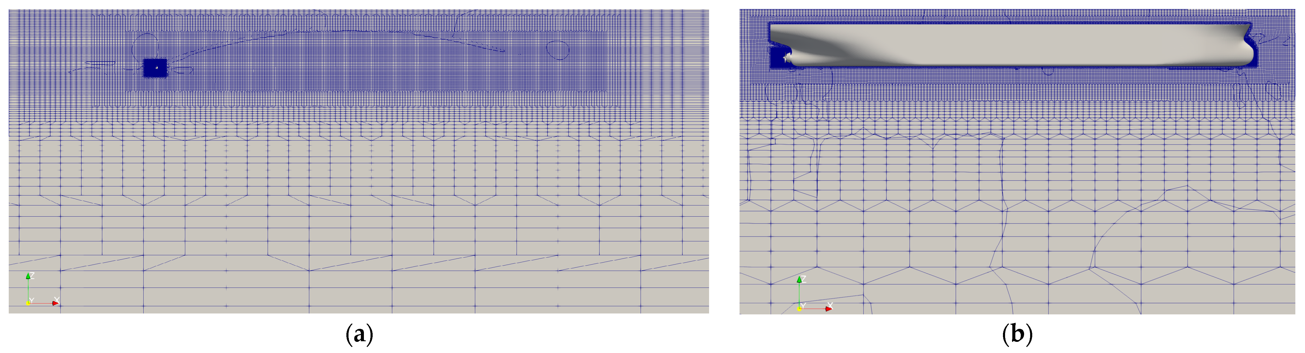
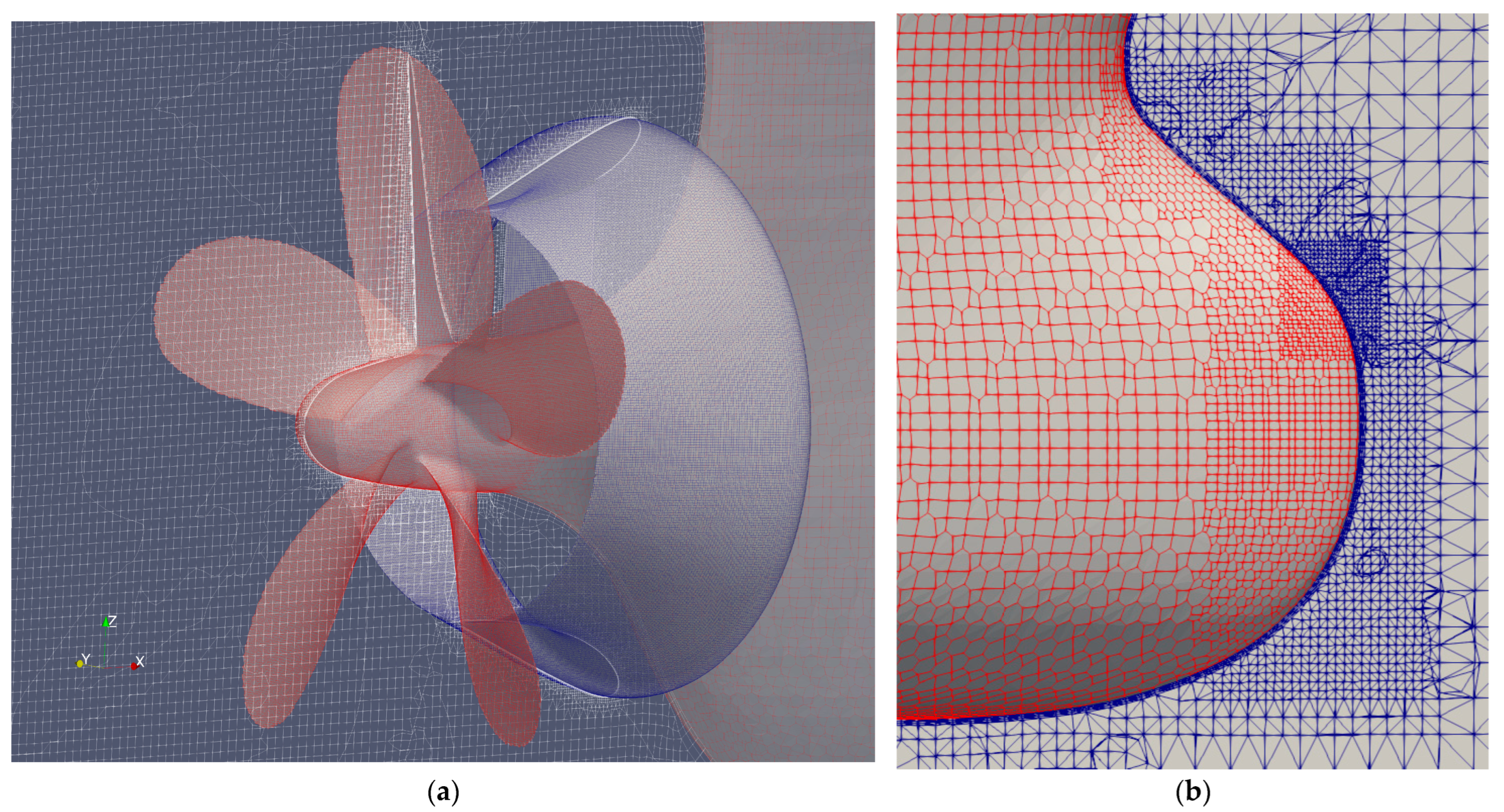
2.4. Unstructured Grid Generation

Constant grid spacing along x–y plane on far field boundaries is applied (Figure 3). A denser grid is allocated toward the free surface vertically based on the geometric distribution. Figure 4 indicates that the Cartesian grid generates finer and finer grids around the ship’s body by six levels from the far field. As mentioned in the previous Section 2.3, the OPT grid in Figure 4a is built by removing the ship hull and duct from the self-propulsion grid in Figure 3b and Figure 4b. The body-fitted grid is constructed as the zoom-in view around the ship stern and bow in Figure 5 as an example. Figure 5 also lists the grid building result of the coarse, medium, and coarse grids for the self-propulsion requested by the V and V analysis. The result is in Section 3.1. Finally, the unstructured grid is built by a polyhedral element with arbitrary polygonal faces. The face number, the edge number, and the alignment of the face are unlimited in OpenFOAM. The element majority is hexahedron. The other polygon is split or degenerated from hexahedra, e.g., the face becomes line, or the line becomes points. Those polygonal elements include tetrahedral wedges, two kinds of pentahedron: prism and pyramid, and two kinds of tet: tetrahedron and tetrahedral wedge.

The layered grids attached on the solid surface to resolve the boundary layer flow can be observed in Figure 6. The layer number of layered grids is 3 on the hull, 4~5 on the duct, and 4 on the propeller. To form a good quality body-fitted (surface) grid and layered grid, an additional grid refinement is added for self-propulsion (Figure 5 left column) in the stern region. As a result, the complicated and delicate geometry details of the stern shape, duct, and propeller are captured in Figure 6a. Those appendages are, relatively, much smaller than the hull body. The stern is characterized by a blunt and curvy lower bottom and sharp upper part toward the centerline plane. A series of grid refinement is also arranged along the bulbous bow (see Figure 5, right column, and Figure 6b). This is required because the propeller has very different feature edges compared with the other parts of the ship. The layered grid generation is influenced by the propeller appearance, and results in low coverage. This bow refinement is unnecessary in the resistance test. The stern refinement is excluded in the resistance test without the duct. In the OPT, the Cartesian meshing method and (stern) grid refinement are inherited from the self-propulsion test. Consequently, the grid generation result around the propeller is shown in Figure 7.

Between two nearby different grid densities, i.e., coarse to medium, and medium to fine grids, the refinement ratio $\sqrt{2}$ is recommended by ITTC 75-03-01-01 [36] along the x, y, and z directions, respectively. Due to the unstructured grid, the increase ratio of the total grid number N_total as close as possible to $\sqrt{8}$ ($=\sqrt{2}\times \sqrt{2}\times \sqrt{2}$) is attempted.

Table 2. Total grid number for T2015 cases.

	Case 1.1	Case 1.2	OPT	Case 1.6
Coarse grid	321,463	581,168	493,679	790,082
Medium grid	1,245,900	1,547,393	1,422,479	2,125,520
Fine grid	2,263,181	3,989,685	3,733,057	5,192,505

and

Table 3. Total grid number for optimal duct simulations.

	Resistance		Self-Propulsion
	NACA 7908	NACA 6.3914	NACA 7908	NACA 6.3914
Coarse grid	551,138	551,677	765,272	763,202
Medium grid	1,481,464	1,488,405	2,071,378	2,073,981
Fine grid	3,886,754	3,886,754	5,073,662	5,083,935

list the N_total of the main cases in this work. In the resistance test, N_total for coarse, medium, and fine grids = 0.32 M (million), 1.2 M, and 2.3 M without duct (T2015 case 1.1); 0.58 M, 1.5 M, and 4.0 M with the original duct (T2015 case 1.2). For the OPT, N_total = 4.9 M, 1.4 M, and 3.7 M. In the self-propulsion test with the original duct (T2015 case 1.6), N_total = 0.79 M, 2.1 M, and 5.2 M with the average y+ = 11.5 on the hull, 1.54 on the duct, and 4.42 on the propeller. Since there is no experiment for our optimal ducts, the grid sensitivity, i.e., only the verification of V and V, is analyzed in Section 3.6. The geometry difference between two optimal ducts is subtle, so that their N_total are close to each other. For the resistance test, N_total = 0.55 M, 1.5 M, 3.9 M; 0.76 M, 2.1 M, 5.1 M for self-propulsion.

3. Results

3.1. V and V (Verification and Validation)

The resistance, OPT, and self-propulsion simulations for the T2015 cases are verified and validated, as shown in

Table 4. V and V results.

	Case 1.1	Case 1.2	OPT (J = 0.4)		Case 1.6
	1000CT	1000CT	KT	KQ	1000CT	KT	KQ
S1	4.3642	4.3272	0.2160	0.03079	5.0053	0.2375	0.02762
S2	4.4031	4.3989	0.2108	0.02976	5.0474	0.2344	0.02759
S3	4.6327	4.6671	0.2022	0.02870	5.5656	0.2131	0.02587
D	4.289	4.263	0.2214	0.02871	4.762	0.233	0.0295
${\epsilon }_{21}$	0.03884	0.07164	$-$0.0052	$-$0.0103	0.04211	$-$0.00313	$-$0.000023
${\epsilon }_{32}$	0.22967	0.26818	$-$0.0087	$-$0.0106	0.51815	$-$0.02132	$-$0.001727
$R_G$	0.16912	0.26713	0.5982	0.9679	0.08128	0.1471	0.01361
E%D	$-$1.76%	$-$1.51%	2.43%	−7.25%	$-$5.11%	$-$1.96%	6.37%
Ug	0.05562	0.05801	0.04351	135%	0.12496	0.09756	0.07219
Ud	1%	1%	Not provided	Not provided	1%	Not provided	Not provided
Ui	0.00046	0.00108	7.8$\times {10}^{-5}$	6.01$\times {10}^{-5}$	0.0026	0.0108	0.00738
Uv	5.6516%	5.8877%	4.4199%	135%	12.5385%	9.8163%	7.2567%

. CT, KT, and KQ are the hull resistance with or without duct, propeller thrust, and torque coefficient. D, the experimental value, and its uncertainty, Ud, are provided by T2015 [1]. Si with i = 1, 2, 3 is the simulation value for the fine, medium, coarse grid. The error E%D is defined as

$$E\mathit{\%}D = (D - S1)/D$$

(1)

$$R_G={\epsilon }_{21}/ {\epsilon }_{32} = (S2 - S1)/(S3 - S2)$$

(2)

The grid convergence is estimated by Equation (2), in which 0 < $R_G$ < 1 indicates that the grid independence is verified for all cases with the monotonic convergence in Table 4. This means that, as the grid number increases, the difference between the results of two nearby grid sizes tends to decrease. Grid uncertainty Ug is evaluated by the V and V theory suggested in ITTC 75-03-01-01 [36]. The iterative uncertainty Ui is calculated by the difference between the maximal and minimal values of the S1 iteration oscillation divided by the mean value of S1. Since all Uv =$\sqrt{{Ug}^2+{Ud}^2+{Ui}^2}$ >|E%D|, the validation is achieved conclusively. The fine grids are used in the following analysis.

The OPT experimental data of the JBC propeller are also provided by T2015 along with case 1.6 [1], but $U_D$ is not provided, so assume $U_D=0$ here. The OPT V and V analysis is only conducted for the advance coefficient J = 0.4 close to the value determined by the thrust identity method referring to the KT of case 1.6.

In Table 4, the $K_T$ and CT errors are around 2%. The propeller behind the hull increasing the hull resistance also increases the over-predicted CT error to 5%. However, the $K_Q$ error is larger (6~7%), and OPT $U_V$ is more than 100% in particular. This is because the coarse grid (S3) results in a very small $K_Q$ error, almost zero, but as the grid number increases, the error magnitude increases, i.e., deviates from the experimental data, and it turns from the over-prediction (S3, S2) to under-prediction (S1). In fact, ${\epsilon }_{21}$~${\epsilon }_{32}$~$-$0.01 (almost zero) and $R_G$~1 provide insight into the $K_Q$ being almost completely converged, i.e., the $K_Q$ barely changes as the grid number increases.

For different J values, the OPT simulation result including $K_T$, $K_Q$, and propeller efficiency η are listed in

Table 5. OPT result.

J	${\mathit{K}}_{\mathit{T}}$	$10{\mathit{K}}_{\mathit{Q}}$	η	$\mathit{E}\mathit{\%}\mathit{D} \mathit{of} {\mathit{K}}_{\mathit{T}}$	$\mathit{E}\mathit{\%}\mathit{D} \mathit{of} 10{\mathit{K}}_{\mathit{Q}}$	E%D of η	Average y+
0.15	0.3023	0.3839	0.1880	2.87%	$-$5.78%	8.19%	4.98
0.25	0.2675	0.3526	0.3019	3.67%	$-$4.90%	8.17%	5.00
0.35	0.2337	0.3238	0.4020	3.01%	$-$6.28%	8.75%	5.03
0.4	0.2160	0.3078	0.4466	2.45%	$-$7.22%	9.02%	5.07
0.45	0.1975	0.2905	0.4869	1.74%	$-$8.32%	9.29%	5.12
0.55	0.1588	0.2506	0.5549	$-$0.72%	$-$10.83%	9.12%	5.23
0.65	0.1177	0.2072	0.5877	$-$5.85%	$-$16.59%	9.21%	5.32
0.75	0.0711	0.1571	0.5405	$-$15.86%	$-$28.36%	9.74%	5.42

with the error against the experimental data. From the open water curves plotted in Figure 8, the experimental and numerical curves share a similar trend, and both point out the highest η at J = 0.65. Basically, the error appears the lowest, less than 2% at J = 0.45 for $K_T$, which is also a switch point from (lower J) over- to (higher J) under-prediction. On the contrary, all $K_Q$ is over-predicted, and the error increases from about 6% to 30% as J increases. As also listed in Table 5, the average y+ increases, corresponding to a thicker boundary layer, as J increases. This implies that, on the propeller foil section, the lift is predicted well but poorly for the drag related to the wall function not suitable for propeller rotational flow in high J. All η errors are less than 10%, with an increasing trend following the J increment.

3.2. Duct Design by Resistance Test

The resistance reduction Rd is defined as:

$$\mathit{Rd} (\%)={\displaystyle \frac{1000C{T}_{with duct}-4.3642}{4.3642}}\times 100\%,$$

(3)

where 4.3642 is the S1 value of case 1.1 in Table 4.

The foil section of the axisymmetric duct is designed by the NACA 4-digits series. The optimal AOA for NACA 4420 (the original section) was found to be 7.06 deg in [35] from 20.06 deg proposed by T2015 [1] for the original duct. Our AOA is defined from the propeller shaft axis with the fixed foil trailing edge, i.e., the duct exit radius does not change. Thus, the 7.06 deg AOA is fixed in this study. In this design stage, the foil section is adjusted from NACA 4420 targeting the maximum Rd, i.e., minimum total resistance, and the optimization step follows as below:

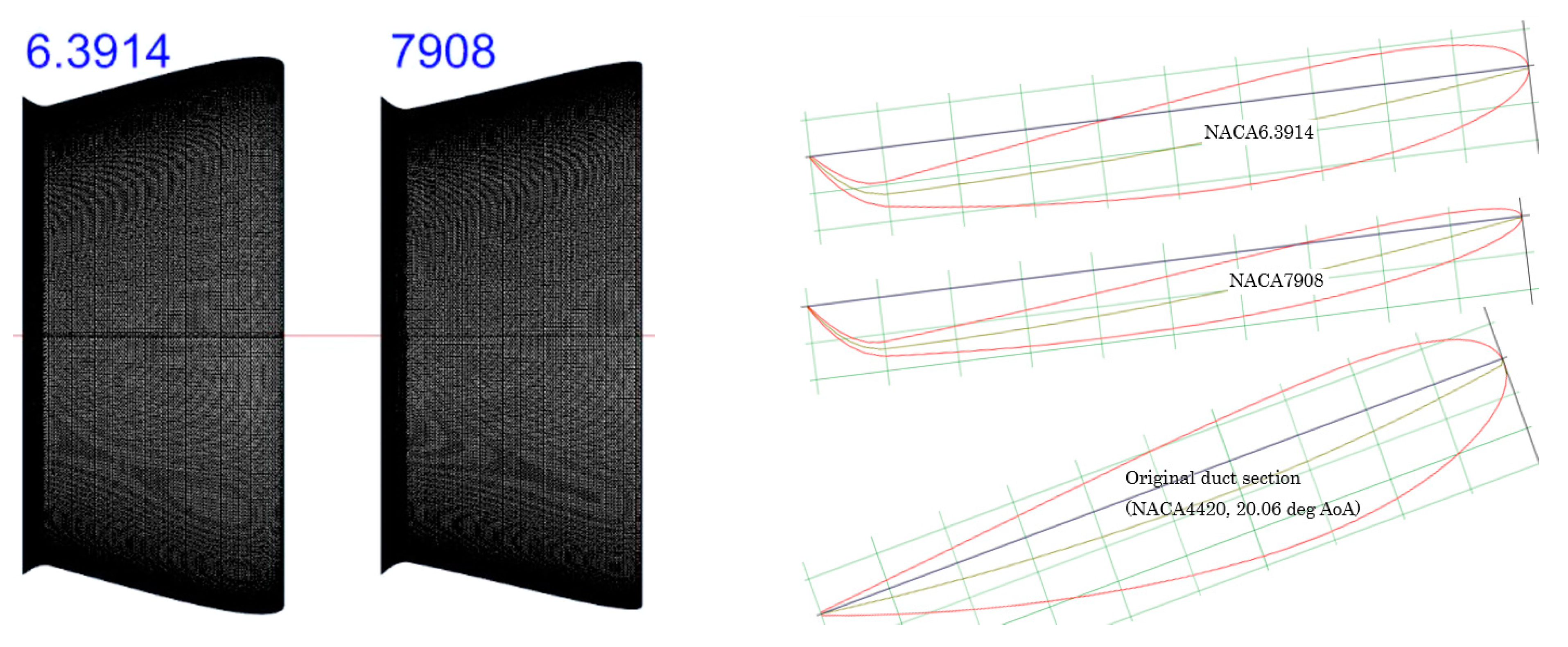
• Maximum camber, e.g., NACA m420 series. Test m = 1~9 and found NACA 6.320 and NACA7420 the best;
• Location of the maximum camber. Test NACA6.3p20 and 7p20 with p = 1~9 and found p = 9 the best for both;
• Maximum thickness. Test NACA 6.39xx with xx = 8~23 and 79xx with xx = 4~24.

Consequently, the NACA 6.3914 and 7908 are concluded as the optimal ducts. Compared to the original duct, both ducts provide 2.8% resistance reduction. Figure 9 shows the history of each optimization step. Figure 10 plots the geometry of the NACA 6.3914 and 7908 ducts, and compared their sections with the original duct. Next, the self-propulsion performance affected by both ducts will be analyzed and investigated.

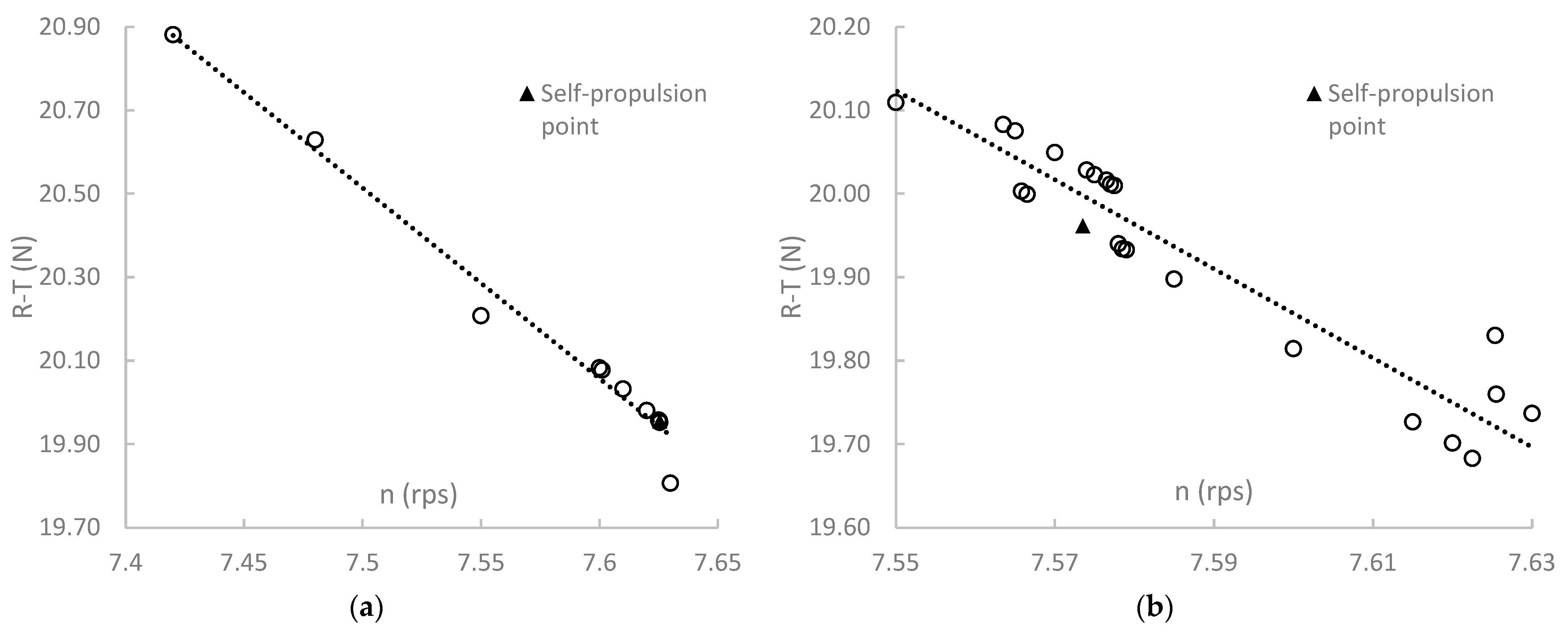
3.3. Self-Propulsion Simulation

For self-propulsion performance, the original duct result in

Table 6. CFD self-propulsion performance.

	Original Duct	NACA 7908 Duct	Diff. from Orig.	NACA 6.3914 Duct	Diff. from Orig.
n (rps)	7.5	7.62542	−1.67%	7.5735	$-$0.98%
10KQ	0.276	0.267604	3.12%	0.267699	3.08%
KT	0.238	0.223	6.30%	0.225	5.46%
1000CT	5.005	4.925	1.60%	4.918	1.74%
1$-$w	0.464	0.520	$-$12.07%	0.509	$-$9.70%
1$-$t	0.740	0.730	1.35%	0.732	1.08%
Va	0.546	0.614	$-$12.45%	0.600	$-$9.89%
EHP 1 (W)	19.754	18.911	4.27%	18.902	4.31%
DHP 2 (W)	25.194	25.654	$-$1.83%	25.143	0.20%
THP 3 (W)	12.379	13.479	$-$8.89%	13.144	$-$6.18%
${\eta }_H$	1.596	1.403	12.09%	1.438	9.90%
${\eta }_o$	0.449	0.487	$-$8.46%	0.481	$-$7.13%
${\eta }_D$	0.784	0.737	5.99%	0.752	4.08%
${\eta }_R$	1.094	1.079	1.37%	1.087	0.64%
${\eta }_B$	0.491	0.525	$-$6.92%	0.523	$-$6.52%

¹ EHP = effective horsepower; ² DHP = delivered horsepower; ³ THP = thrust horsepower.

is computed from the case 1.6 S1 result in Table 4. The propeller rotational rate n = 7.5 rps (revolution per sec) is provided by T2015 [1]. The self-propulsion point is searched for the NACA 6.3914 and 7908 ducts individually targeting the SFC (Skin Friction Correction) = 19.9551 N.

When the resistance (R) including ship hull and stern duct, minus the propeller thrust (T), is approximately close to the SFC value, the ship self-propulsion point is achieved. The searching history of finding self-propulsion point is shown in Figure 11. The convergence trend is clear for NACA 7908 duct, instead the R$-$T of NACA 6.3914 duct with more curvy and thicker section (see Figure 10) oscillates within a band of approximate 0.08N.

The self-propulsion performance parameters in Table 6 are calculated based on the KT and KQ curves fitted from the OPT experimental data provided by T2015 [1]:

$$KT=-0.1633{\ast J_a}^2-0.2694\ast J_a+0.3553,$$

(4)

$$10KQ=-0.0956{\ast J_a}^3-0.1549{\ast J_a}^2-0.1947\ast J_a+0.3959,$$

(5)

where $J_a$ = U/(n∗D) is the advance coefficient with propeller diameter D and n (rps).

In Table 6, the difference from the original duct is calculated as:

$$\mathrm{Diff}. \mathrm{from} \mathrm{Orig}. (\%)={\displaystyle \frac{(\mathrm{O}\mathrm{r}\mathrm{i}\mathrm{g}\mathrm{n}\mathrm{a}\mathrm{l} \mathrm{d}\mathrm{u}\mathrm{c}\mathrm{t} \mathrm{v}\mathrm{a}\mathrm{l}\mathrm{u}\mathrm{e})-(\mathrm{O}\mathrm{p}\mathrm{t}\mathrm{i}\mathrm{m}\mathrm{a}\mathrm{l} \mathrm{d}\mathrm{u}\mathrm{c}\mathrm{t} \mathrm{v}\mathrm{a}\mathrm{l}\mathrm{u}\mathrm{e})}{(\mathrm{O}\mathrm{r}\mathrm{i}\mathrm{g}\mathrm{n}\mathrm{a}\mathrm{l} \mathrm{d}\mathrm{u}\mathrm{c}\mathrm{t} \mathrm{v}\mathrm{a}\mathrm{l}\mathrm{u}\mathrm{e})}}\times 100\%.$$

(6)

Table 6 shows some and similar improvements for self-propulsion performance are provided by installing NACA 7908 and 6.3914. The hull resistance (CT) decreases by 1.6 and 1.7%. The propeller thrust coefficient decreases by 6 and 5% to reach a higher self-propulsion point near 7.6 rps (1% higher than 7.5 rps for the original duct ). The 3% lower torque indicates the propeller rotates easier behind two ducts. In particular, the NACA 6.3914 requires slightly less delivered horsepower. Basically, the lower effective horsepower and higher thrust horsepower correspond to the lower hull resistance (CT) and higher propeller rps, respectively. The propeller behind-hull efficiency ${\eta }_B$ increases by around 7%. Both ducts produce obvious flow acceleration, achieving around a 10% higher effective wake factor (1$-$w) corresponding to faster propeller advance velocity Va.

The main efficiency improvement of the optimal ducts is propeller-related, such as ${\eta }_B$ and ${\eta }_o$ (open water efficiency). The hull efficiency ${\eta }_H$, quasi-propulsive efficiency ${\eta }_D$, relative rotative efficiency ${\eta }_R$, and thrust deduction factor (1$-$t) are not improved. Since the ship hull and propeller geometry are not modified, the traditional ship propulsion efficiency definition might not be fair for an energy saving device [11].

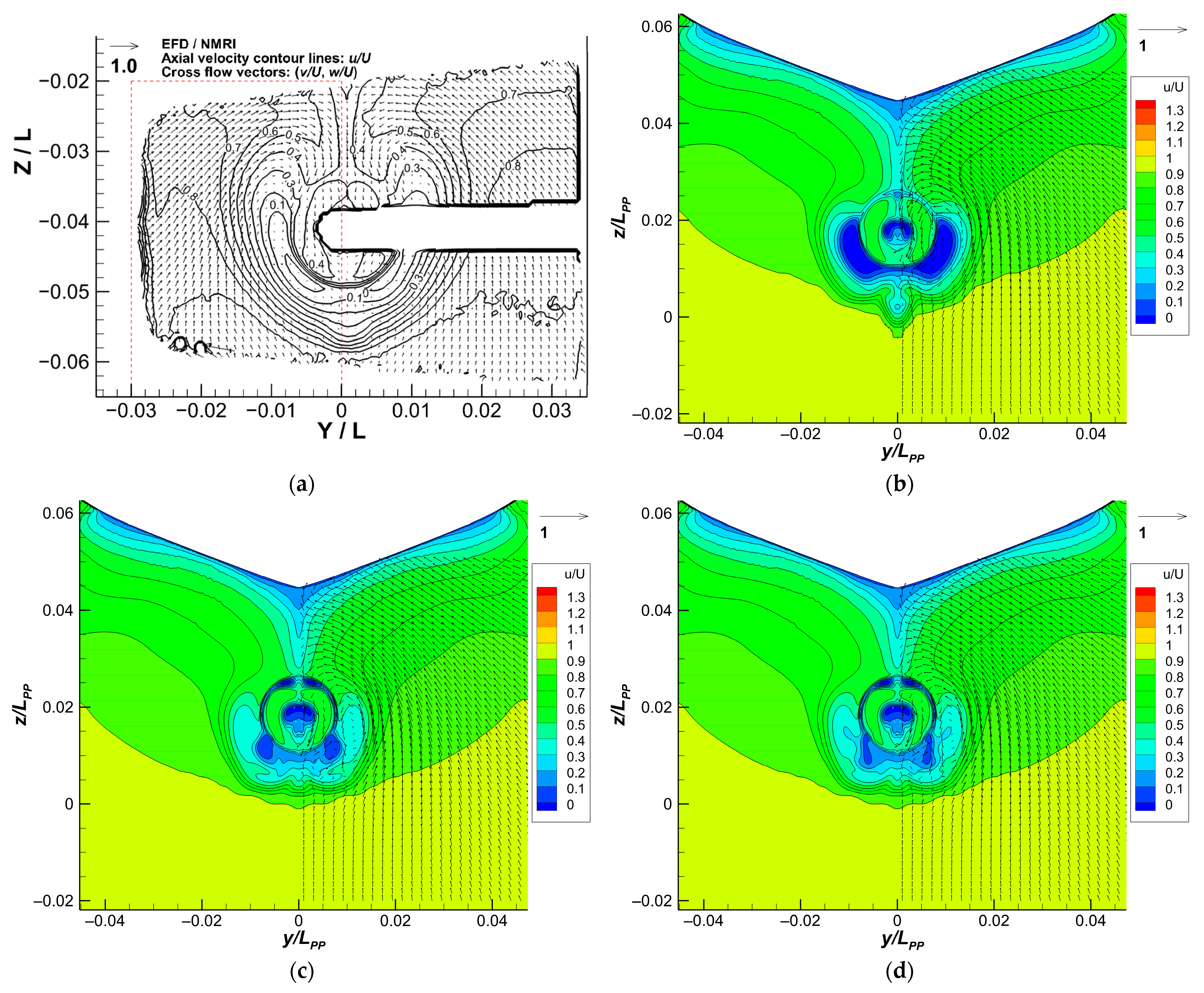
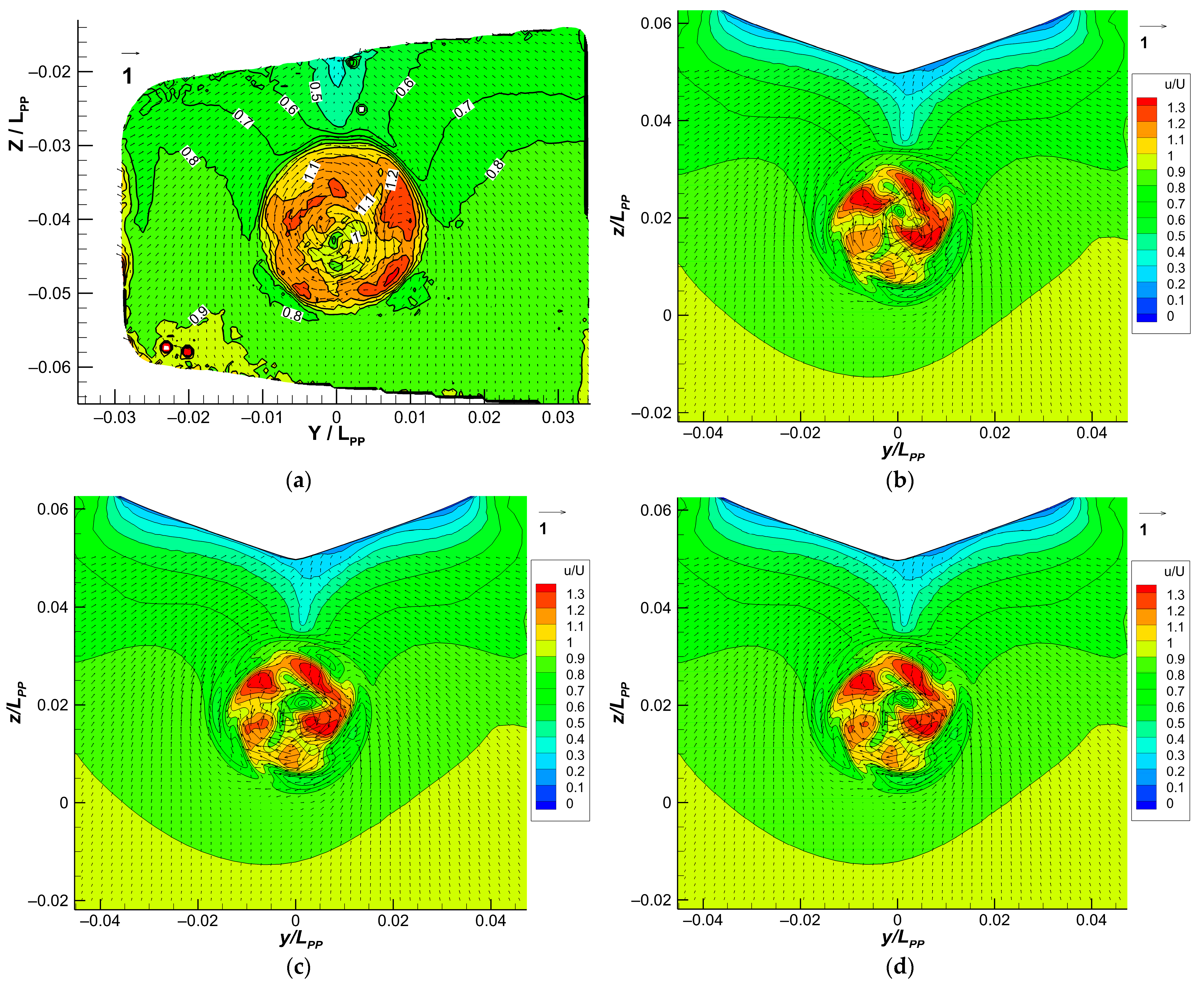
3.4. Nominal and Propeller Wake Field

For nominal wake, Figure 12a,b show the large flow separation, i.e., u/U (non-dimensional axial flow velocity) < 0, behind the lower half part of the original duct presented in both experiments and our fine grid simulation. Figure 12c,d reveal that both optimal ducts effectively reduce the flow separation area. In fact, their u/U would not be less than 0 in this region, explaining the resistance reduction. Although both optimal ducts provide the same resistance reduction (2.8%, see Section 3.2), their velocity profile patterns are slightly different. For the NACA 6.3914 duct, the width of the u/U = 0~0.1 region around (y/L_PP, z/L_PP) = ($\pm$0.0065, 0.008~0.014) is thinner in y direction, but a small branch of the u/U = 0.2~0.3 region extends from ($\pm$0.008, 0.013) to ($\pm$0.01, 0.015) which does not exist for the NACA 7908 duct. However, the small flow separation is caused behind the upper half of both ducts, i.e., the wake becomes slightly worse in this part of the flow field.

The high axial velocity (u/U > 1.2) distributed in the upper and starboard sides of the propeller wake behind the hull are measured by the experiment in Figure 13a and captured by our fine grid simulation in Figure 13b. The starboard portion corresponds to the interaction of the right rotating propeller and stern upward flow causing a higher relative velocity and leading to a higher propeller inflow velocity. The upper port side portion is induced by the right rotating propeller and bilge vortex downward flow, e.g., the vectors around (y/L, z/L) = ($-$0.006, $-$0.034) in Figure 12a. The larger area of the u/U > 1.3 distribution for CFD results corresponds to the over-predicted propeller KT (case 1.6 S1 in Table 4). This reflects the ship’s stern wake as not being well equalized or uniformed for the propeller inflow. By contrast, for the optimal ducts, a small portion of the u/U > 1.2 can be observed in Figure 13c,d in the port-side lower part of the propeller wake. In other words, the propeller loading, i.e., propeller wake distribution or output, is more circumferentially even. This confirms that the more uniform wake and better wake equalization are produced by the two optimal ducts. The lower torque in Table 6 also supports this observation. Two ducts result in the slight difference here. For the NACA 6.3914 duct, the u/U > 1.2 is more scattered, e.g., (y/L_PP, z/L_PP) in the lower port side around ($-$0.05~$-$0.01, 0.015), and upper starboard side around (0.01, 0.02).

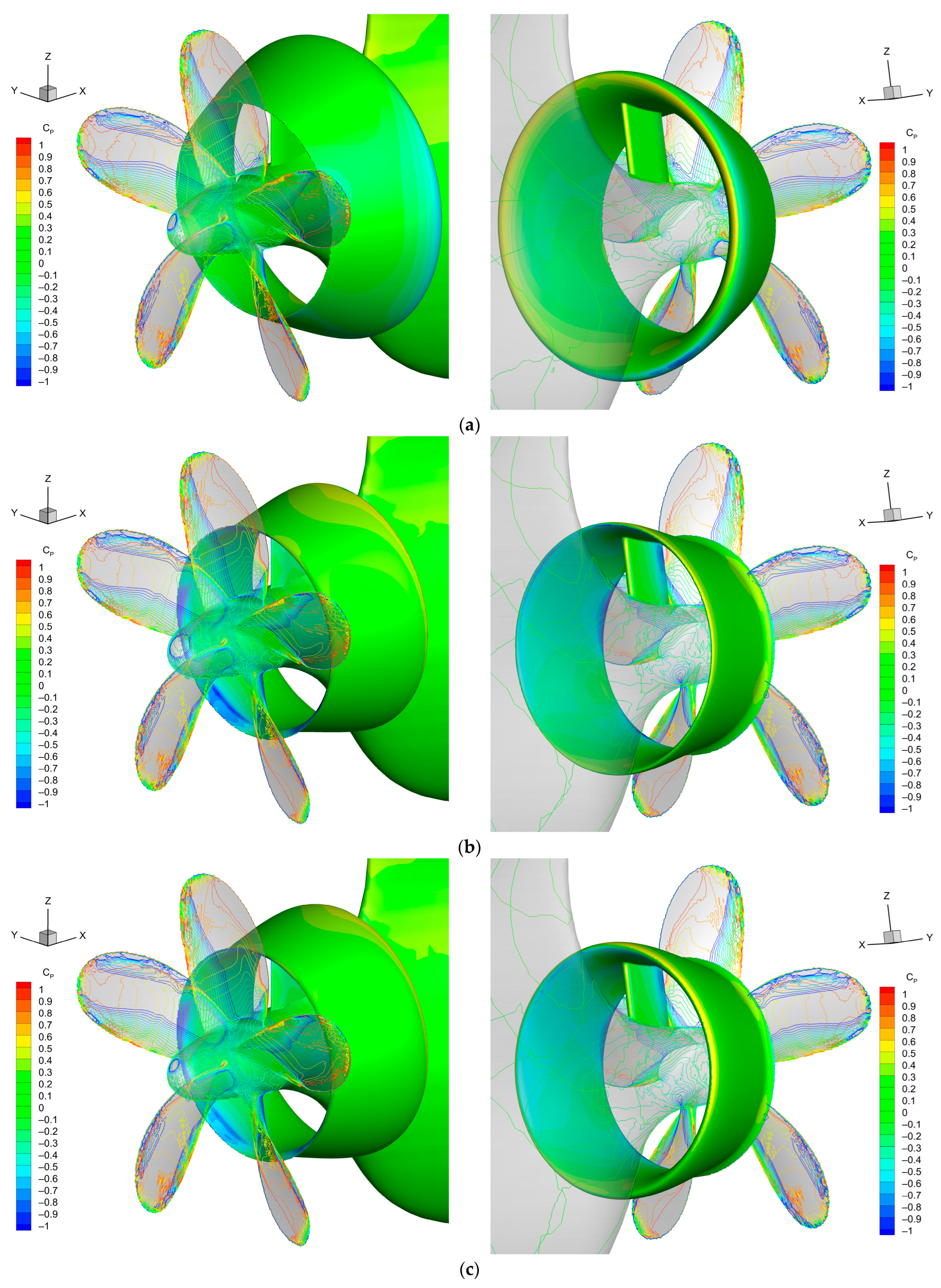
3.5. Pressure Coefficient Distribution

Figure 14 plots the pressure coefficient (C_P) distribution on the ship stern, propeller, and duct, including the original and two optimal ducts: the NACA7908 and 6.3914 ducts. The benefit of the optimal ducts for energy saving and propulsion performance is explored in detail in the figure. On the outer surface of the original duct (the pressure/back side), the low and negative C_P (in blue) occurs near the leading edge. The high and positive C_P (in red) appears near the leading edge of the inner surface of the original duct (the suction/face side). It turns out that the pressure difference on the original duct causes resistance, i.e., the resultant force pointing backward against the propeller’s thrust direction or ship’s advancing direction. Instead, on both optimal ducts, the high and positive C_P (in red) is located near the leading edge of the outer surface (the pressure/back side). Also, the low and negative C_P (in blue) is observed near the trailing edge of the inner surface (the suction/face side), i.e., the bending outward exit. As a result, the pressure difference on the optimal ducts yields the additional thrust. In other words, the foil lift contributes to a forward component.

The propeller thrust is produced by the high and positive C_P (in red) on the propeller face and the low and negative C_P (in blue) on the propeller back.

Some sight deterioration of C_P is found locally for two optimal ducts in comparison of the original duct. The C_P around the trailing edge of the strut is negative and lower (in blue) for both optimal ducts, but for the original duct, the C_P is about zero (in green). The core of the low and negative C_P (in blue) on the propeller hub surface is larger for the NACA7908 duct.

3.6. Grid Sensitivity for Optimal Ducts

In this section, the grid sensitivity is examined since the experiment is unavailable currently for the optimal ducts. The fine grid result (S1) is assumed to be close enough to the experimental value in order to estimate the grid uncertainty, Ug. The results for the resistance and self-propulsion simulations are presented in

Table 7. Grid sensitivity for the optimal ducts.

	NACA7908 Duct				NACA6.3914 Duct
	Resistance Test	Self-Propulsion Test (Propeller Rotational Rate = 7.5 rps)			Resistance Test	Self-Propulsion Test (Propeller Rotational Rate = 7.5 rps)
	1000CT	1000CT	KT	KQ	1000CT	1000CT	KT	KQ
S1 = D *	4.2431	4.9098	0.2232	0.0265	4.2429	4.9193	0.2250	0.0266
S2	4.3130	4.9327	0.2192	0.0262	4.3083	4.9311	0.2191	0.0262
S3	4.5724	5.4231	0.1974	0.0243	4.5282	5.4413	0.1988	0.0244
${\epsilon }_{21}$	0.06993	0.04657	$-$0.00403	$-$0.00033	0.06535	0.01176	$-$0.00591	$-$0.00045
${\epsilon }_{32}$	0.25934	0.02284	$-$0.02183	$-$0.00189	0.21991	0.51024	$-$0.02028	$-$0.00174
$R_G$	0.26966	0.04657	0.18471	0.17502	0.29715	0.02305	0.29179	0.25990
Ug	0.05620	0.11907	0.10008	0.07425	0.04621	0.12667	0.08078	0.06089
Ui	0.00120	0.00173	0.00887	0.01054	0.00119	0.00142	0.00026	0.00025
Uv	5.6206%	11.905%	10.008%	7.425%	4.6211%	12.667%	8.078%	6.089%

* It is assumed, since the experiment is unavailable currently.

. All $R_G$ = 0~1 indicates the grid convergence is confirmed as monotonic convergence. Compared to the Uv of cases 1.1 and 1.6 in Section 3.1 (Table 4), the Uv values show the same level of uncertainty. For resistance simulation, Uv is 5~6%. In the self-propulsion simulation, Uv is 12~13% for the resistance, 8~10% for the propeller thrust, and 6~7% for the propeller torque.

4. Discussion

The CFD method for resistance, open water propeller, and self-propulsion simulation is verified and validated in the presented work and then is extended to design the JBC’s stern duct. The duct section is designed by using the NACA 4-digits foil series profile. The optimal duct with the NACA 7908 or 6.3914 sections is found with a 2.8% reduction for bare hull resistance. In the self-propulsion point, the propeller thrust decreases by 6 and 5% to achieve the 1.6 and 1.7% lower hull resistance. Eventually, the 7 and 6% higher propeller behind-hull efficiency and 10% higher effective wake factor are obtained. Both ducts achieve energy saving by decreasing effective horsepower by 4.3%. In other words, by installing one of the ducts, less power output is required to propel the ship in the design speed. Other than slightly less delivered power is required, the NACA 6.3914 duct also performs slightly better for the local flow field phenomena. Since the flow separation in the nominal wake is improved, the more uniform propeller wake is caused by the better wake equalization presenting a more uniform propeller inflow.

In the presented work, the stern duct was optimized for a particular ship model, JBC, in a calm water condition. Since the JBC is a bulk carrier, the optimal duct and design outcome might be only suitable for or recommended for a similar hull form, i.e., full hull form. For slimmer ship types, e.g., container ships, the stern duct needs another optimization. Also, a ship sailing in the sea encounters waves and requires it to perform turning or zig-zags. In addition, the surface roughness of a ship’s hull changes continuously along its service life due to fouling, corrosion, deformation, etc. However, a smooth surface is assumed in this study. Therefore, the seakeeping and maneuvering performance, and proper roughness of the ship with ESDs, should be considered and designed accordingly. The above-mentioned challenges and limitations are our future work.

References

1. JAPAN Bulk Carrier (JBC), Tokyo 2015 a Workshop on CFD in Ship Hydrodynamics. Available online: https://t2015.nmri.go.jp/jbc_gc.html (accessed on 28 February 2025).
2. Schneekluth Hydrodynamik GmbH. Available online: https://www.schneekluth.com/en/ (accessed on 4 April 2025).
3. Sanoyas Shipbuilding Co., Ltd. Available online: https://www.sanoyas.skdy.co.jp/technology (accessed on 4 April 2025).
4. Gougoulidis, G.; Vasileiadis, N. An Overview of Hydrodynamic Energy Efficiency Improvement Measures. In Proceedings of the 5th International Symposium on Ship Operations, Athens, Greece, 28–29 May 2015. [Google Scholar]
5. Lee, J.-T.; Kim, M.-C.; Suh, J.-C.; Kim, S.-H.; Choi, J.-K. Development of a preswirl stator-propeller system for improvement of propulsion efficiency: A symmetric stator propulsion system. J. Soc. Nav. Archit. Korea 1992, 29, 132–145. [Google Scholar]
6. Park, S.; Oh, G.; Rhee, S.H.; Koo, B.Y.; Lee, H. Full scale wake prediction of an energy saving device by using computational fluid dynamics. Ocean Eng. 2015, 101, 254–263. [Google Scholar] [CrossRef]
7. Guiard, T.; Leonard, S. The Becker Mewis Duct®-Challenges in Full-Scale Design and new Developments for Fast Ships. In Proceedings of the 3rd International Symposium on Marine Propulsors, Launceston, Australia, 5–8 May 2013. [Google Scholar]
8. Elangovan, M. Hydrodynamic Energy Devices to Improve the Efficiency of Propulsion System in AUVs. Int. Res. J. Adv. Sci. Hub 2020, 2, 18–22. [Google Scholar] [CrossRef]
9. Andersson, J.; Shiri, A.A.; Bensow, R.E.; Yixing, J.; Chengsheng, W.; Gengyao, Q.; Deng, G.; Queutey, P.; Xing-Kaeding, Y.; Horn, P.; et al. Ship-scale CFD benchmark study of a pre-swirl duct on KVLCC2. Appl. Ocean Res. 2022, 123, 103134. [Google Scholar] [CrossRef]
10. Falchi, M.; Aloisio, G. On the Effect of Energy Saving Devices on the Wake Hydrodynamics of a Bulk Carrier Model. In Proceedings of the Thirty-First International Ocean and Polar Engineering Conference, Rhodes, Greece, 20–25 June 2021. [Google Scholar]
11. Schuiling, B.; van Terwisga, T. Hydrodynamic working principles of Energy Saving Devices in ship propulsion systems. Int. Shipbuild. Prog. 2017, 63, 255–290. [Google Scholar] [CrossRef]
12. Narita, H.; Yagi, H.; Johnson, H.D.; Breves, L.R. Development and full scale experiences of a novel integrated duct propeller. SNAME Trans. 1981, 89, 319–346. [Google Scholar]
13. Kitazawa, T.; Hukino, M.; Fujimoto, T.; Ueda, K. Increase in the propulsive efficiency of a ship with the installation of a nozzle immediately forward of the propeller. J. Kansai Soc. Nav. Archit. Jpn. 1982, 184, 73–78. [Google Scholar]
14. Schneekluth, H. Wake equalizing duct. Nav. Archit. 1986, 103, 147–150. [Google Scholar]
15. Sasaki, N.; Aono, T. Energy saving device “SILD”. J. Shipbuild. Jpn. 1997, 45, 47–50. [Google Scholar]
16. Inukai, Y.; Itabashi, M.; Sudo, Y.; Takeda, T.; Ochi, F. Energy saving device for ship IHIMU semicircular duct. IHI Eng. Rev. 2007, 40, 59–63. [Google Scholar]
17. Mewis, F. A novel power saving device for full form vessels. In Proceedings of the First International Symposium on Marine Propulsors (SMP’09), Trondheim, Norway, 22–24 June 2009. [Google Scholar]
18. Energy-Saving Technology. Available online: https://global.kawasaki.com/en/mobility/marine/technology/energy_saving.html (accessed on 28 February 2025).
19. Schuiling, B. The design and numerical demonstration of a new energy saving device. In Proceedings of the 16th Numerical Towing Tank Symposium (NUTTS 2013), Mulheim, Germany, 2–4 September 2013. [Google Scholar]
20. Menter, F.; Kuntz, M.; Langtry, R. Ten years of industrial experience with the SST turbulence model, in: Turbulence, Heat and Mass Transfer. In Proceedings of the 4th International Symposium on Turbulence, Heat and Mass Transfer, Antalya, Turkey, 12–17 October 2003; pp. 625–632. [Google Scholar]
21. Nicorelli, G.; Villa, D.; Gaggero, S. Pre-swirl ducts, pre-swirl fins and wake-equalizing ducts for the DTC hull: Design and scale effects. J. Mar. Sci. Eng. 2023, 11, 1032. [Google Scholar] [CrossRef]
22. Sakamoto, N.; Kawanami, Y.; Hinatsu, M.; Uto, S. Viscous CFD analysis of stern duct installed on panamax bulk carrier in model and full scale. In Proceedings of the 15th International Conference on Computer and IT Applications in the Maritime Industries, Lecce, Italy, 9–11 May 2016. [Google Scholar]
23. Tahara, Y.; Peri, D.; Campana, E.F.; Stern, F. Computational fluid dynamics-based multiobjective optimization of a surface combatant using a global optimization method. J. Mar. Sci. Technol. 2008, 13, 95–116. [Google Scholar] [CrossRef]
24. Tahara, Y.; Norisada, K.; Yamane, M.; Takai, T. Development and demonstration of CAD/CFD/optimizer integrated simulation-based design framework by using high-fidelity viscous free-surface RANS equation solver. J. Jpn. Soc. Nav. Archit. Ocean Eng. 2008, 7, 171–184. [Google Scholar] [CrossRef]
25. Lee, M.-K.; Lee, I. Optimal Design of Flow Control Fins for a Small Container Ship Based on Machine Learning. J. Mar. Sci. Eng. 2023, 11, 1149. [Google Scholar] [CrossRef]
26. Diez, M.; Serani, A.; Campana, E.F.; Goren, O.; Sarioz, K.; Danisman, D.B.; Grigoropoulos, G.; Aloniati, E.; Visonneau, M.; Queutey, P.; et al. Multi-objective hydrodynamic optimization of the DTMB 5415 for resistance and seakeeping. In Proceedings of the 13th International Conference on Fast Sea Transportation (FAST 2015), Washington, DC, USA, 1–4 September 2015. [Google Scholar]
27. Grigoropoulos, G.; Campana, E.; Diez, M.; Serani, A.; Goren, O.; Sariöz, K.; Danisman, D.B.; Visonneau, M.; Queutey, P.; Abdel-Maksoud, M.; et al. Mission-based hull-form and propeller optimization of a transom stern destroyer for best performance in the sea environment. In Proceedings of the VII International Conference on Computational Methods in Marine Engineering (MARINE2017), Nantes, France, 15–17 May 2017. [Google Scholar]
28. Guo, J.; Zhang, Y.; Chen, Z.; Feng, Y. CFD-based multi-objective optimization of a waterjet-propelled trimaran. Ocean Eng. 2020, 195, 106755. [Google Scholar] [CrossRef]
29. Wie, D.-E.; Kim, D.-J. The Design Optimization of a Flow Control Fin Using CFD. J. Soc. Nav. Archit. Korea 2012, 49, 174–181. [Google Scholar] [CrossRef]
30. Vesting, F.; Bensow, R. Propeller Optimisation Considering Sheet Cavitation and Hull Interaction. In Proceedings of the Second International Symposium on Marine Propulsors (SMP’11), Hamburg, Germany, 15–17 June 2011. [Google Scholar]
31. Vázquez-Santos, A.; Camacho-Zamora, N.; Hernández-Hernández, J.; Herrera-May, A.L.; Santos-Cortes, L.d.C.; Tejeda-del-Cueto, M.E. Numerical Analysis and Validation of an Optimized B-Series Marine Propeller Based on NSGA-II Constrained by Cavitation. J. Mar. Sci. Eng. 2024, 12, 205. [Google Scholar] [CrossRef]
32. Zhai, S.; Jin, S.; Chen, J.; Liu, Z.; Song, X. CFD-based multi-objective optimization of the duct for a rim-driven thruster. Ocean Eng. 2022, 264, 112467. [Google Scholar] [CrossRef]
33. Nguyen, V.T.; Chandar, D. Ship specific optimization of pre-duct energy saving devices using reduced order models. Appl. Ocean Res. 2023, 131, 103449. [Google Scholar] [CrossRef]
34. Furcas, F.; Vernengo, G.; Villa, D.; Gaggero, S. Design of wake equalizing ducts using RANSE-based SBDO. Appl. Ocean Res. 2020, 97, 102087. [Google Scholar] [CrossRef]
35. Wu, P.-C.; Chang, C.-W.; Huang, Y.-C. Design of Energy-Saving Duct for JBC to Reduce Ship Resistance by CFD Method. Energies 2022, 15, 6484. [Google Scholar] [CrossRef]
36. ITTC Recommended Procedures and Guidelines 7.5-03-01-01: Uncertainty Analysis in CFD Verification and Validation Methodology and Procedures. Available online: https://ittc.info/media/4184/75-03-01-01.pdf (accessed on 20 September 2008).
37. Rusche, H. Computational Fluid Dynamics of Dispersed Two-Phase Flows at High Phase Fractions. Ph.D. Thesis, Imperial College London, London, UK, 2002. [Google Scholar]
38. Holzmann, T. The numerical algorithms: SIMPLE, PISO and PIMPLE. In Mathematics, Numerics, Derivations and OpenFOAM®; Holzmann CFD: Loeben, Germany, 2006; pp. 93–121. [Google Scholar]
Figure 1. Ship and propeller model [1]: (a) the hull with bulbous bow; (b) propeller and stern duct.
Inventions 10 00032 g001
Figure 2. Computational domain size: (a) resistance simulation; (b) self-propulsion simulation.
Inventions 10 00032 g002
Figure 3. Grid distribution on far field boundaries: (a) resistance (the hull surface is in red color); (b) self-propulsion test.
Inventions 10 00032 g003
Figure 4. Grid refinement levels: (a) open-water propeller; (b) self-propulsion.
Inventions 10 00032 g004
Figure 5. The unstructured grid topology around the ship bow (right) and stern (left) for self-propulsion simulation: (a) coarse grid; (b) medium grid; (c) fine grid.
Inventions 10 00032 g005
Figure 6. Layered and surface grids (fine grid for self-propulsion simulation): (a) around the stern, propeller and duct; (b) on the bow.
Inventions 10 00032 g006
Figure 7. Grids around the open-water propeller (fine grid): (a) back surface; (b) y = 0 plane.
Inventions 10 00032 g007
Figure 8. Propeller open water curves (EFD = Experimental Fluid Dynamics).
Inventions 10 00032 g008
Figure 9. NACA 4-digits design for the duct section: (a) NACA m420 series; (b) NACA6.3p20 and 7p20; (c) NACA6.39xx and 79xx.
Inventions 10 00032 g009
Figure 10. NACA6.3914 and NACA7908 ducts, and their sections compared with the original duct.
Inventions 10 00032 g010
Figure 11. Self-propulsion point searching history: (a) NACA 7908 duct; (b) NACA6.3914.
Inventions 10 00032 g011
Figure 12. Nominal wake velocity field (u/U, v/U, w/U) at x / L p p = 0.9843 (between duct and propeller): (a) experimental data [1] for the original duct; (b) original duct; (c) NACA7908 duct; (d) NACA6.3914 duct. The fine grid result (S1) is shown for the CFD results.
Inventions 10 00032 g012
Figure 13. Axial velocity distribution (u/U) and cross flow vectors (v/U, w/U) of propeller wake behind the hull at ship AP ( x / L p p = 1.0): (a) experimental data [1] for the original duct; (b) original duct; (c) NACA 7908 duct; (d) NACA 6.3914 duct. The fine grid result (S1) is shown for the CFD results.
Inventions 10 00032 g013
Figure 14. Pressure coefficient distribution on stern, duct, and propeller surface: (a) original duct; (b) NACA7908 duct; (c) NACA6.3914 duct. The fine grid result (S1) is shown here.
Inventions 10 00032 g014