Abstract
Individual road mobility comes with two major challenges: greenhouse gas emissions related to global warming and chemical pollution. For the pollution reduction in the spark ignition engine vehicle, the standard and reliable aftertreatment technology is the three-way catalytic converter (TWC). However, the TWC starts to convert once an optimal temperature, usually known as the light-off temperature, is reached. There are many methods to reduce the warm-up period of the TWC, among which is using a burner. The initial question underlying this study was to see if the use of a relatively straightforward extra-combustion device mounted upstream the TWC, without complex elements, was able to serve the purpose of reducing the light-off time. Consequently, an original burner was designed and investigated numerically via the CFD method and experimentally via measurements of the temperature evolution within a TWC, along with the emissions specific to the burner’s operation. The main findings of this study are: (1) the CFD-based examination is a good way to decide on how to achieve the so-called fit-for-purpose internal aerodynamics of the burner (i.e., to obtain a homogeneous mixture) and (2) to reach the light-off temperature, conventionally taken as 500 K, the burner was operated for 5.2 s, i.e., 3.6 g of gasoline injected, 2.7 g of CO2 and 1.351 g of CO, respectively, emitted. Moreover, this study identified measures for improving the burner’s design as well as an enhanced procedure for the burner’s operating control both aiming to produce a cleaner combustion during the TWC pre-heating.
1. Introduction
Individual road mobility is paramount for human society. The passenger car became not only a means of ensuring door-to-door mobility, but also the very expression of the freedom of movement, hence its importance. However, the passenger car is also one of the major contributors to environmental degradation, as is well known. Pollution (unburnt hydrocarbon—UHC, carbon monoxide—CO, nitrogen oxides—NOx, particulate matter—PM) and carbon dioxide (CO2), emitted by their internal combustion (IC) engines, have become a growing global concern. A solution to this problem was to replace the thermal propulsion ensured by the IC engine with the electric propulsion ensured by the battery electric vehicles (BEVs). Some parts of the world even issued regulations to favor BEVs, as is the case in Europe—for instance, see the Green Deal’s Fit-for-55 package, which “makes reaching the EU’s climate goal of reducing EU emission by at least 55% by 2030 a legal obligation” [1]. This regulation also sets a target of 100% carbon emission reduction for 2035, meaning that “all new cars and vans placed on the market in the EU from 2035 should be zero-emission vehicles (ZEV)” [2], based on a tank-to-wheel approach, which also means BEVs. Nonetheless, the worldwide electrification of individual road mobility via BEVs is challenging and will not happen overnight. Thus, for the time being, the internal combustion (IC) engine will continue to be used worldwide for individual road mobility either as standalone powerplants (ICEV—internal combustion engine vehicle) or as part of hybrid electric vehicles (HEVs). Obviously, the discussions are about the IC engine as a solution for sustainable road mobility, and consequently the IC engine should be as efficient and as ecologic as possible—an engine with “zero impact emissions”, as defined in [3,4]: (1) its pollutants are reduced to such a low level that it does not have a negative impact on air quality anymore and (2) its net CO2 emissions are zero (all local CO2 are compensated by CO2 capture elsewhere). To address this environmental challenge related to the ICEV, researchers are expected to develop even more efficient and cleaner technologies.
For the pollution reduction in the spark ignition engine vehicle (SIEV), the classic and reliable aftertreatment technology is the closed loop controlled three-way catalytic converter (TWC), which uses noble metal catalysts such as platinum (Pt), palladium (Pd) and rhodium (Rh) to facilitate the conversion of the aforementioned pollutants into harmless substances, such as CO2, H2O, N2 and O2. The conversion efficiency or the effectiveness of the catalytic converters for a given pollutant (x) is shown below:
where x may be any of the regulated gaseous pollutants, e.g., UHC, CO, NO, NO2; Exhaust_out and Engine_out are the pollutants at the tailpipe and produced by the engine (i.e., downstream and upstream the catalytic converter).
There are many studies focusing on the main parameters influencing the effectiveness of the catalytic converters [5,6,7,8,9]: oxygen storage capacity (OSC) of the converter (i.e., adsorption and release of oxygen from the converter’s wash coat), air–fuel ratio (AFR), and catalyst temperature (TTWC) as the bulk temperature of the converter’s monolith. On this theme, the authors of papers [6,7] agreed that OSC is “not prevalent during the warm-up” and, consequently TTWC and AFR would be the main factors to influence conversion efficiency. Hence, as discussed in [5], the effectiveness of the catalytic converter for a given pollutant (x) is the product of two efficiencies, as shown below:
According to [7], both efficiencies introduced in relation (2) can be modelled with Wiebe mathematical functions, typically known as S-shaped curves.
The thermal behavior of the catalytic converter is well described in the paper [5], which is actually based on the papers [6,7]:
- ▪
- Forced convection between the exhaust gas and the monolith, ,
- ▪
- Forced convection between the converter’s outer wall and the ambient air, , and
- ▪
- Exothermic and endothermic catalytic reactions to convert the pollutants, .
So, during the TWC warm-up, Equation (3) gives the rate of TTWC:
where designates rates of heat flow, is the TWC mass, and is the TWC heat capacity at constant pressure.
However, the TWC starts to convert once an optimal operating temperature is reached. This is widely known as the light-off temperature, which based on the considerations presented above, varies with the gaseous pollutants. In the literature, most frequently, this temperature is referred to in a generic way, as the temperature corresponding to a catalyst effectiveness of 50% (T50); this temperature would be approximately 500 K, according to [5,10,11,12,13,14]. Obviously, one may consider any conversion efficiency for this light-off temperature, e.g., T90, meaning the temperature at which 90% conversion is reached for any chemical species, as used in paper [15], which, among other findings, shows that T90 for CO is nearly insensitive to lambda (i.e., AFR made dimensionless by stoichiometric conditions) between 0.977 and 1.005, while “T90 for NO is constant for lambda inferior to 0.995 but increases by more than 200 °C for lambda values between 0.995 and 1.001, and 90% conversion is not achieved at any temperature for lambda higher than 1.001”.
The above considerations convey the idea that the main problem with the TWC is the warm-up phase, i.e., the period after the engine’s cold start, until the TWC reaches this temperature threshold called light-off. It is therefore vital to have the TWC light off as quickly as possible and this is harder as the ambient temperature decreases. This problem has been well known from the beginning of the pollution reduction via the TWC and, consequently various measures are used to address it, some of them already introduced in mass production.
Back in 1994, paper [12] argued that although TWC “has already achieved a high level of development, further improvements are still required in order to reliably fulfil the future standards”. At present, this statement is still valid, especially because of the extreme tightening of the automotive pollution regulation. For instance, the objective of the future Euro7, as declared in the papers [4,16,17], is to be able to label the IC engine “zero impact emissions” to avoid banning it out of the European cities. Among the improvements proposed in [12], one may also find measures to reduce the warm-up period of the TWC:
- Thermally insulated exhaust pipes (not currently used in mass production).
- Converters installed as near to the engine as possible (today, this is called closed-coupled TWC and it is used in mass production).
- Injection of air upstream the TWC relying on fuel post-oxidation (this was and is still used in some mass production applications).
- Electrically heated catalytic converter, EHC (nowadays, it seems to be a potential solution for the HEV considering the frequent stop-and-start sequences of the IC engine and especially the on-board source of electricity; however, the reliability of the electrical metallic structure of the heated disc, which is in continuous contact with very hot exhaust gas from the IC engine is a potential blocking point).
- Fuel afterburner chamber and burner (the last two never entered the production phase).
Fuel post-oxidation benefits in terms of light-off time were assessed by a CFD investigation in paper [18]. The authors explored the effects of air injection into the exhaust on the light-off time, while each cylinder was operated with rich mixture, showing that “the observed temperature increase is obtained at the expenses of about 10% in terms of fuel consumption”. The increased fuel consumption while using air injection for the enhancement of fuel post-oxidation generated by the engine operation in the rich mode was also reported in paper [19].
According to Langen et al. [12], the difference between the “fuel afterburner chamber” and the “burner” is that the former is burning fuel coming out from the engine, which has to be ran richer (hence, the term after-burner), while the latter has its own fuel supply. Obviously, both require an ignition source and a blower/air pump to provide the oxygen supply. Chan et al. [13] listed the same measures aiming to expedite the reaching of light-off temperature but discussed the solutions generated by different strategies used while calibrating the engine.
Returning to the heating time of the TWC, as discussed in [4], complying with Euro7 may require having the TWC already heated up even before the IC engine starts (i.e., pre-heating). If so, the only solutions able to provide this standard are burner technology and EHC, the latter, however, being reserved for the HEV (due to the need for sufficient onboard electric power, e.g., 2.0 kW, 4.0 kW or even 8.6 kW, coupled with a 45 kg/h mass air flow rate, as explored in [20]).
As regards the burner technology for TWCs, as already mentioned, it is not a new idea. Nonetheless, further to our literature survey, this technology is mainly cited in SAE papers from the 1990s, e.g., [12,21,22]. In more recent years, in the main scientific stream, this solution is rather mentioned in review papers, such as [10], which do not provide many details about it and also quote SAE papers from the 1990s. Our extensive search on this particular subject revealed two recent papers [23,24] dealing with the numerical assessment of an aftertreatment system equipped with a burner, another article [4] presenting, among other details, clear results of using a so-called “additional fuel burner” in the attempt to achieve the “zero-impact emissions” engine and only one work [25] dedicated to a burner development for light-off speed-up of an aftertreatment system in gasoline engine (like the older paper [21]).
This paper also focuses on presenting an original burner designed to reduce the TWC light-off time. Previously, as presented in [26], our focus was on experimentally investigating the effect of a burner on the light-off performance of a TWC by using a retrofitted commercial WebastoTM water heater to warm the vehicle cabin, to de-ice the vehicle windows and to pre-heat water-cooled vehicle engines. The findings of this research were valid; however, the retrofitted heater was not able to heat-up the pre-catalyst in reasonable time because of the insufficient air mass flow ensured by the heater’s fan. Consequently, the original burner presented in this paper was designed to ensure a sufficient air mass flow and thus, a rapid heat-up of the pre-catalytic converter, in order to ensure a high aftertreatment effectiveness once the SI engine is turned on, without using the different penalizing strategies used while calibrating the engine (i.e., spark retardation, lambda-split or mixture leaning, etc., as presented in [13]). More precisely, the scope of this work was to develop an original extra-combustion device mounted upstream the TWC (i.e., a burner) characterized by the so-called fit-for-purpose internal aerodynamics able to quickly generate a homogeneous and ignitable mixture only relying on a simple design not using relatively complex elements imported from the aeronautical burner application, such as the ones presented in paper [25].
Accordingly, the remainder of this paper is structured as follows: first, the design of the burner’s combustion chamber is presented, with a description of the internal aerodynamics of the burner based on CFD results; then, the investigation of the burner’s operation, i.e., (1) the burner’s control oriented to quickly achieve an ignitable mixture in the combustion chamber and (2) measurements of the temperature evolution within a two-part TWC (a smaller pre-catalytic converter and a main catalytic converter), along with the emissions specific to the burner’s operation.
2. Burner Design and CFD Investigation
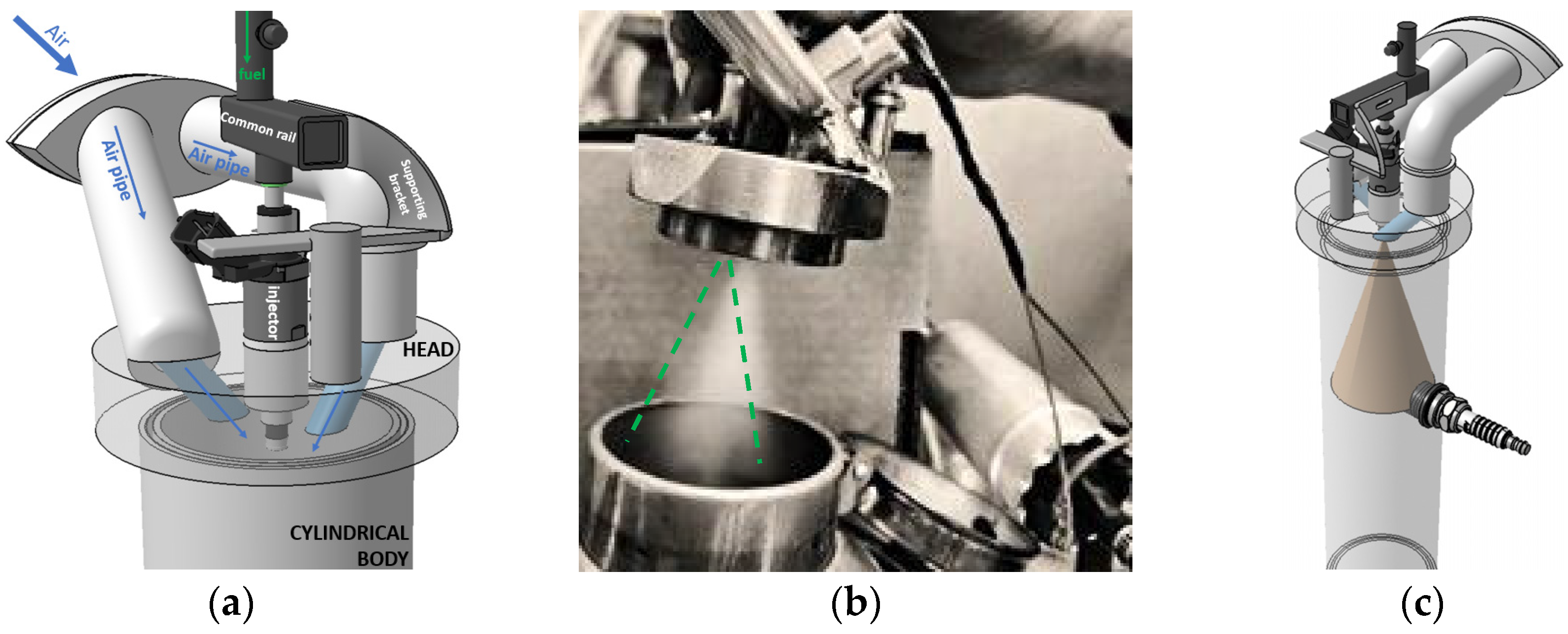
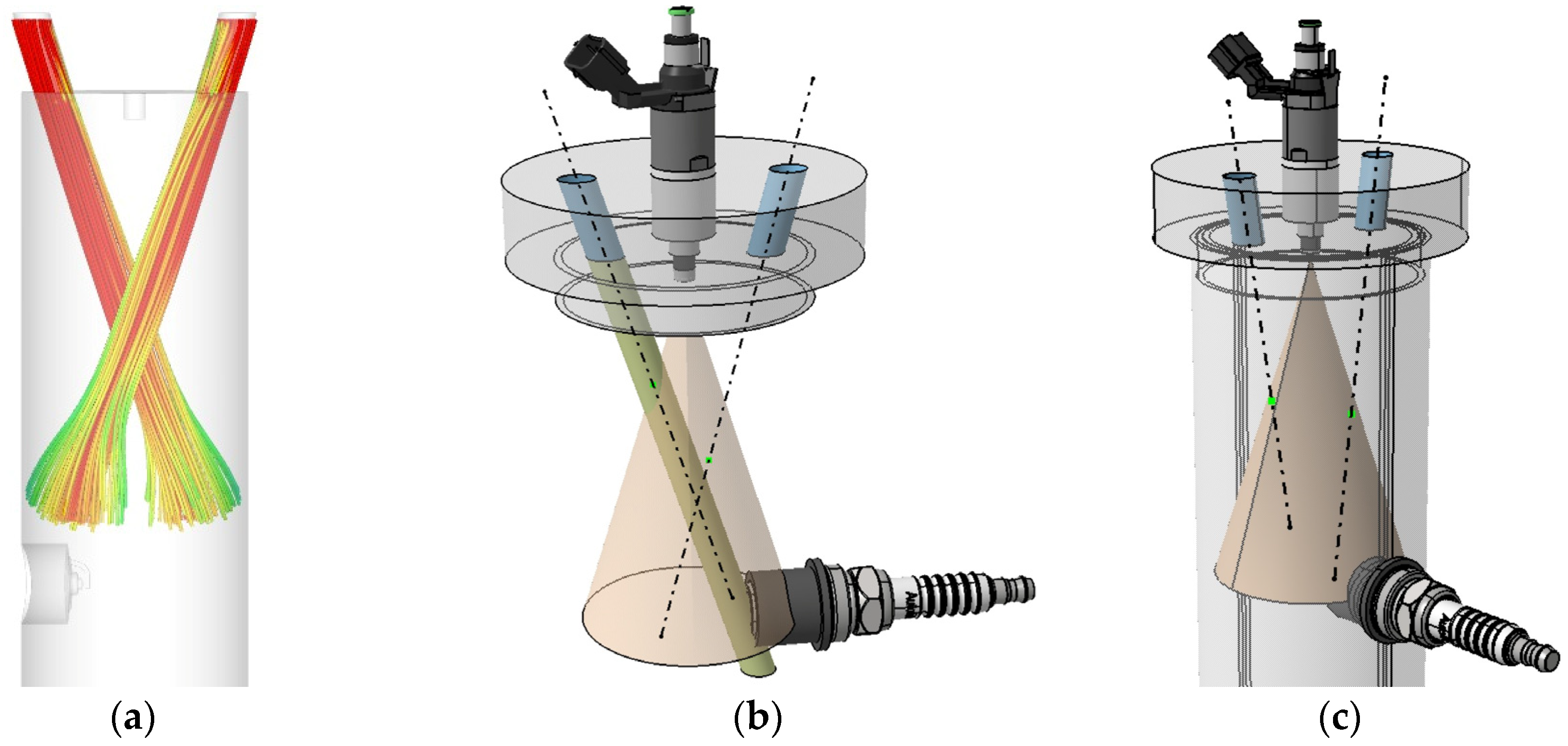
As mentioned before, when designing the burner’s combustion chamber the focus was on how to obtain a homogeneous and ignitable mixture mainly relying on the airstream inside the burner’s body. As shown in Figure 1a, the burner comprises two parts, which are welded together: (1) the head containing the injector with its fueling parts, two air pipes with their corresponding ducts through the head and (2) the body, which has a constant cylindrical section (purely for reasons of simplicity).
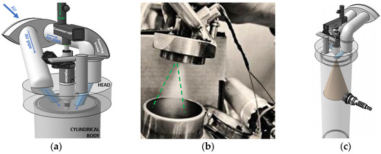
Figure 1.
Burner’s design: (a) main parts; (b) cone angle of injected fuel from the experiment; (c) positioning of the spark plug.
As seen in Figure 1c, the positioning of the spark plug was set based on the experimentally estimated cone angle of the injected fuel (34°—see the green dashed line in Figure 1b); thus, its vertical location on the cylindrical body was decided to be right where this cone touches the inner cylindrical surface. The hypothesis is that it is in this way that the flame occurrence is maximized. Evidently, the experimentally estimated injected fuel cone was necessary since the technical specifications of the injector were not provided by its manufacturer.
In order to obtain a homogeneous mixture, as mentioned before, the focus was on how to achieve the so-called fit-for-purpose internal aerodynamics.
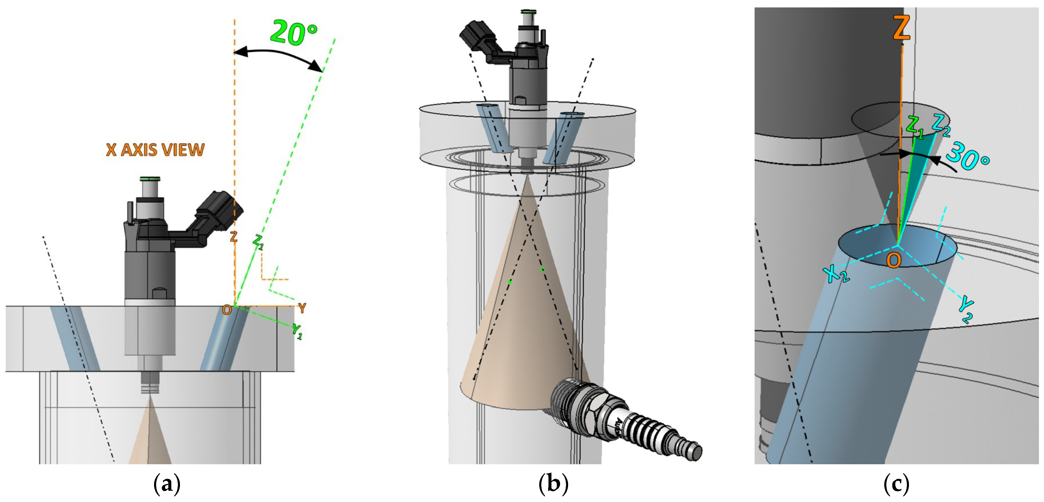
Thus, the directions of the two ducts through the burner’s head were designed, first, to conveniently intersect the injected fuel cone (see the arbitrary 20° angle in Figure 2a and, hence the two green dots in Figure 2b, which are the intersection points) and, second, to generate an air swirl motion (i.e., a rotation of the air around a vertical axis—see the arbitrary 30° angle in Figure 2c). On the latter, as there are two ducts through the head, two swirls were planned, both in the same direction, one following the other.

Figure 2.
Burner’s initial design for homogeneous mixture: (a) ducts inclination to achieve air intersection with the fuel cone; (b) intersection between air and fuel cone; (c) ducts inclination to achieve the swirl motions.
This is the first design iteration and the physical prototype was manufactured as such (see Section 3). Furthermore, to draw conclusions regarding the aerodynamics inside the burner, generated by the design explained above, a CFD simulation was performed.
The CFD simulation is ran in AVL FIRETM 2022 R1 software (Graz, Austria), which is based on the finite volume approach and is a 3D RANS-based (Reynolds-average Navier–Stokes) cold simulation of the air flow at 40 kg/h (boundary condition imposed at the inlet faces of the two air ducts) for 5 s with a time step of 0.05 s, using the k-ζ-f model. According to [27,28], this turbulence model produces reasonable results with good accuracy in resolving the dominant structures of the turbulent flow and gives a better prediction of flow separation and reattachment. The simulation is called cold because the burner is not fired.
The selection of the mesh size is the result of several simulations aiming to achieve the independence of the numerical solution with respect to the grid. Subsequently, to analyze the influence of the mesh/grid on the numerical solution, different values for the maximum cell size were used (0.7, 0.8, 0.9, 1.0 mm). Evidently, the finer the mesh, the higher the computational time. Table 1 shows the values of some physical parameters, calculated after the 5 s of simulation with a step of 0.05 s, as well as the CPU time specific to the workstation used (2.3 GHz, Intel Xeon 36 cores, 128 GB RAM).

Table 1.
Influence of the mesh on the numerical solution for the k-ζ-f turbulence model.
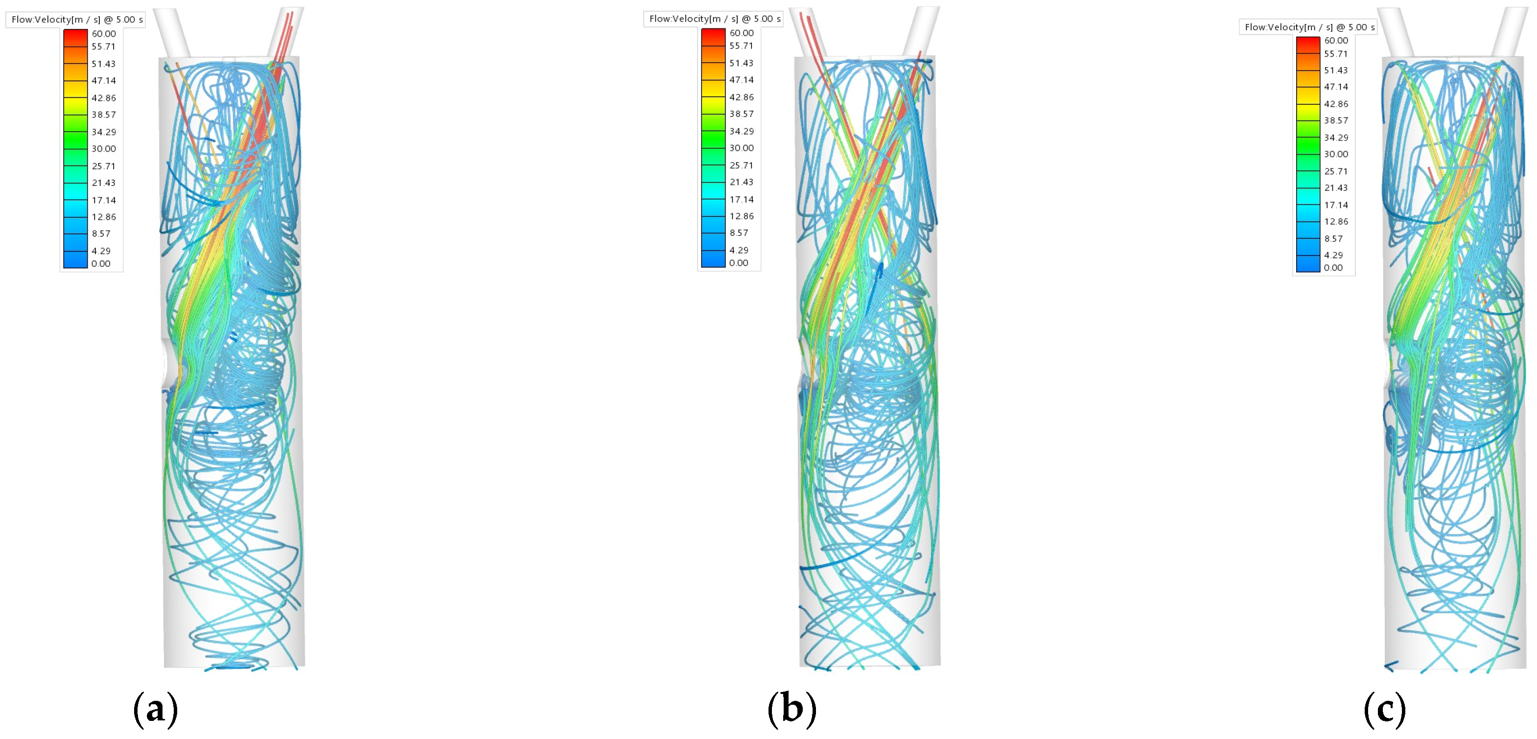
Since at this stage, the focus was mainly on predicting the large-scale air structures and because decreasing the maximum cell size from 1.0 to 0.7 did not result in significant changes in these structures, Figure 3, the maximum cell size used for this CFD RANS- based study was 0.7 mm.
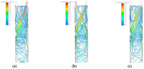
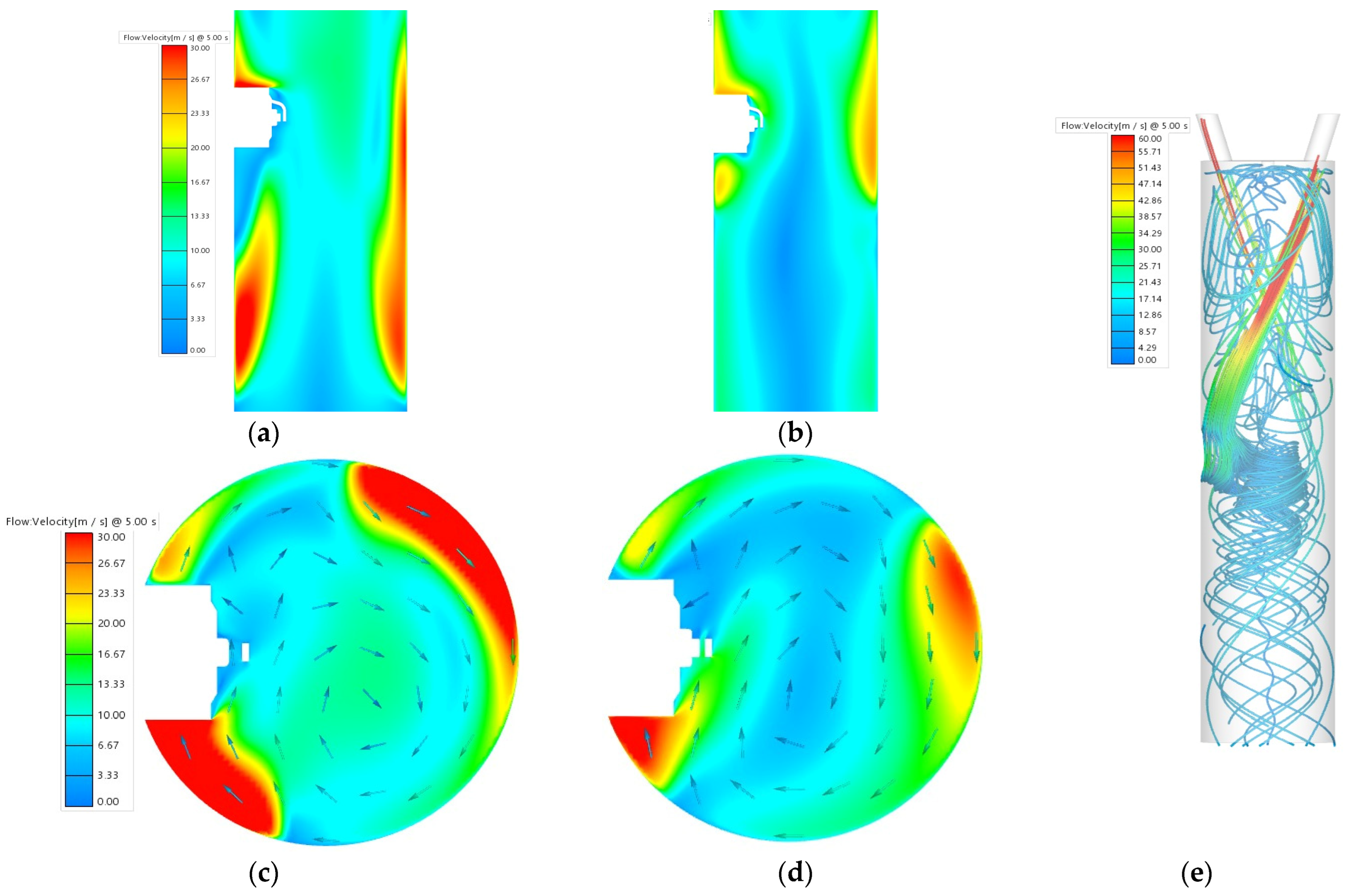
Figure 3.
Burner’s internal aerodynamics at 5s via the k-ζ-f model: (a) max. cell size: 0.9; (b) max. cell size: 0.8; (c) max. cell size: 0.7. NB. Spark plug location is visible at the left.
Choosing a suitable turbulence model is always a challenging task for the scientific community. As per [29], the scientific community argued that most turbulence models are validated for specific well-defined test cases, but it is not certain whether they are also valid for other type of flows generated by complex geometries where the flow might be different. In terms of the turbulence models that can be used with the RANS approach, each has advantages and disadvantages. For instance, according to [30], the k-ε model is “relatively simple to implement, leads to stable calculations that converge relatively easily and makes reasonable predictions for many flows, but is valid just for fully turbulent flows, and predicts the swirling and rotating flows rather poorly”.
Based on the above considerations, another simulation was conducted, this time using the k-ε turbulence model. Thus, we were able to analyze comparatively the CFD results (i.e., using the same software, mesh size, initial and boundary conditions, based on the same RANS approach, only changing the turbulence models: k-ζ-f vs. k-ε). Table 2 shows the figures resulted from this k-ε simulation. When comparing with the data from Table 1, one may see that (1) when using the k-ζ-f model, the computing time was higher and (2) while the maximum and mean 2D flow velocities are within the same order for both models, the mean TKE is significantly higher in the k-ε case.
Table 2.
Influence of the k-ε model on the simulation.
Figure 4a–d shows the flow velocity fields obtained with both turbulence models in the vertical and horizontal planes containing the spark plug. While the maximum cell size was 0.7 mm, the area around the spark plug was refined and the smallest cell size reached 0.0437 mm between the two electrodes. The vectors displayed in Figure 4c,d are projected in plane.
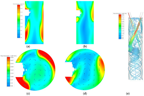
Figure 4.
Burner’s internal aerodynamics at 5s: (a) vertical plane with k-ζ-f model; (b) vertical plane with k-ε; (c) horizontal plane with k-ζ-f model; (d) horizontal plane with k-ε; (e) streamlines generated by the k-ε model.
As seen in Table 1 and Table 2, the maximum 2D flow velocities are over 130 m/s, while Figure 4 shows values up to 30 m/s. Since Figure 4 was focused on the flow in the spark plug region, where the velocities are much lower than the maximum value, the color mapping range was conveniently chosen to discern more efficiently between different velocities in this area. The same was performed for Figure 3 and Figure 4e, which presents the streamlines generated by the flow at 5 s, because the maximum flow velocities occur in the two entering air ducts from the burner’s head.
When analyzing comparatively the results of the two turbulence models, Figure 4a–d, one may see that (1) both models predict horizontal large-scale vortexes rotating in the same direction (clockwise) and (2) the predicted velocities are globally lower for the k-ε model. This analysis of the flow around the spark plug is of interest because the flame kernel development initiated by the spark produced between the electrodes is influenced by the flow: either the flow is too intense and the kernel may be extinguished or the flow is too low, the kernel develops poorly and affects negatively the combustion performance. In the situations presented in Figure 4a–d, the following velocities were obtained between the two electrodes: 14.9 m/s for the k-ε model and 5.7 m/s for the k-ζ-f model. Thus, noticeable difference between the results provided by the two models and somehow, unexpectedly higher for the k-ε model as globally, this model predicts lower velocities (Figure 4 and Table 1 and Table 2). Nonetheless, as seen in Figure 4e, the k-ε model predicts intense rotating flows in the spark plug area, even though, globally, the large-scale structures seem like those presented in Figure 3.
Finally, the conclusion drawn from this CFD investigation is rather of a qualitative kind, meaning that the simulations predict comparable/similar large-scale air structures. As previously discussed, when first designing the air ducts through the burner’s head, the idea was to direct one of the air flows towards the spark plug after hitting the fuel injected cone, Figure 2b, aiming to help flame propagation. As seen in Figure 4a,b, with the current 20° inclination, there is an impact between one of the two main airstreams and the cylindrical wall just above the spark plug, Figure 5a, which lowers the air velocities between the electrodes of the spark plug.

Figure 5.
Burner’s design evolution: (a) exclusive visualization of two main airstreams generated by the initial air ducts—results obtained with k-ζ-f model; (b) different inclination of the ducts; (c) 90° rotation around the burner’s vertical axis of symmetry of the initial air ducts assembly.
The improving ideas that emerged from this study are: (1) to incline the duct responsible for directing the air towards the electrodes so as to achieve this specific goal and to maintain the other duct with the inclinations given in Figure 2 in order to generate a swirl, Figure 5b; (2) to rotate the initial air ducts assembly around the burner’s vertical axis of symmetry in order to avoid blowing towards the electrodes, Figure 5c, in case the conclusion is that the flow at the electrodes’ level is too intense and might extinguish the flame kernel.
To be able to draw more pertinent conclusions, all the design iterations should be complemented with CFD studies aiming to see the air–fuel interaction and the combustion process. The conclusions reached during this CFD investigation may be validated experimentally based on the measured starting delay of the burner, which may be an indication of the right choice for the two air ducts inclinations: the lower the starting delay, the better. This is part of the future works and based on the conclusions of this next CFD study, another prototype will be built.
3. Experimental Setup and Testing Methodology
When designing the burner, the focus was on obtaining a relatively affordable and straightforward extra-combustion device mounted upstream the TWC by relying on existing components on mass-production ICEV, such as the following: an air pump from a SI engine featuring air injection into the exhaust, a standard hot-wire mass air flowmeter (HW MAF), a gasoline injector taken rather from a port-fuel injection (PFI) system than from a gasoline direct injection (GDI) system, a usual spark plug together with its coil and a wide-band lambda probe. Moreover, this investigation’s purpose was also to see if a simple design not using relatively complex elements such as the ones mentioned in [25] (e.g., an injector and a coil able to support high control frequencies, e.g., 200 and, respectively, 250 Hz, “a swirler containing a tiny slot with an optimized shape and location to promote a fast mixture preparation at the spark plug”, a “prefilmer” taken from aeronautical burner applications and “a flame holder”, the second one needing “optimization in relation to the swirler shape”) is able to serve the purpose of rapidly reaching the light-off temperature.
The schema of the experimental setup for laboratory testing is presented in Figure 6.
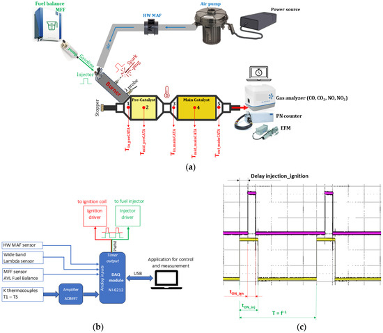
Figure 6.
Schematic of the burner’s lab testing: (a) components and instrumentation; (b) control and measurement; (c) oscilloscope acquired signals of ignition (magenta) and injection (yellow).
The testing methodology first aims to find how quickly the burner starts and then its effect on the heating of a two-part TWC (a smaller pre-catalytic converter and a main catalytic converter), along with the emissions specific to the burner’s operation. Thus, it is about what is usually called “catalyst pre-heating”, i.e., the burner operates before the engine starts—as shown in Figure 6a, where there is no SI engine upstream the TWC and, consequently a stopper is used at the left side of the exhaust line.
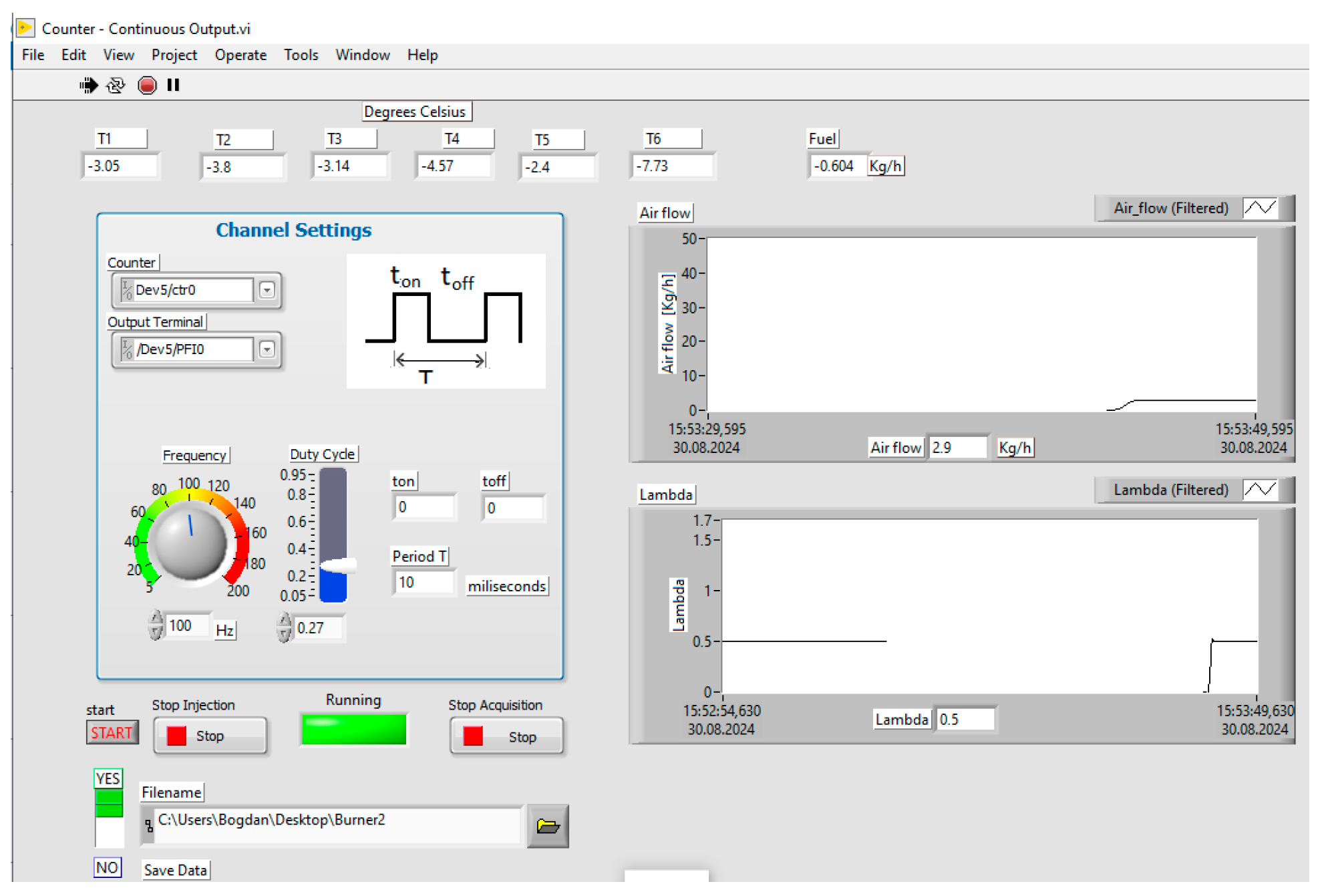
To serve this purpose, first, the air pump was activated and operated at its maximum capacity of 40 kg/h steady flow, and then, the gasoline injection and the spark were activated via pulse-width modulation (PWM), Figure 6c, whereas the quality of the mixture (rich/stoichiometric/lean) was monitored via a wide-band lambda probe. The gasoline was pressurized by a usual electrically actuated pump at 5 bar. The fuel flow rate was adjusted to serve the need to control the mixture quality: rich in the beginning, to facilitate the starting of the burner, then, gradually and manually leaning the mixture (the lambda probe providing the feedback signal). The mass fuel flow rate (MFF) was measured with a usual AVLTM 733S fuel balance (AVL, Graz, Austria). The TWC was instrumented with five K type thermocouples, as shown in Figure 6a. All these signals are controlled by a dedicated LabViewTM (National Instruments, USA) application, communicating with a data acquisition module from National InstrumentsTM—Figure 6b. The software application interface showing how the burner’s operational parameters are controlled is presented in Figure 7. The spark delay time related to the injection time is controlled by an ArduinoTM Uno module, in charge of the ignition coil command.
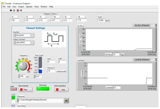
Figure 7.
The software application interface: injection and ignition PWM specific parameters.
As Figure 6a shows, the exhaust emissions related to burner’s operation are measured with an AVLTM PEMS (Portable Emission Measurement System) containing a gas analyzer for CO, CO2, NO and NO2, a particle number (PN) counter able to detect particles with diameters higher than 23 nm and an exhaust flow mass rate (EFM) to express the chemical species in [kg/h] and by integration, in mass over a certain period of time.
4. Experimental Results and Discussion
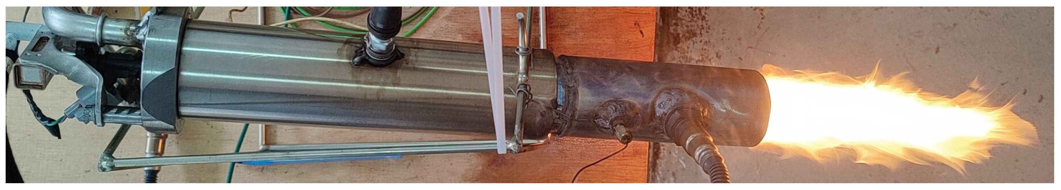
After several attempts to achieve the optimal burner’s starting, finally, the burner’s injection and ignition were actuated as follows: 100 Hz actuating frequency for both signals; 3.7 ms injection duration at the beginning to achieve a rich and ignitable mixture and then, after the starting of the burner, gradually and manually decreasing it to 1.7 ms (thus, leaning the mixture); 3.5 ms actuation duration of the spark plug coil and 0 ms delay between the injection and ignition signals, aiming to produce the spark in a favorable environment (i.e., an ignitable mixture), Figure 6c. A picture with the flame produced by operating the burner as discussed above is presented in Figure 8.
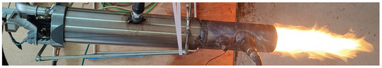
Figure 8.
The burner while operating.
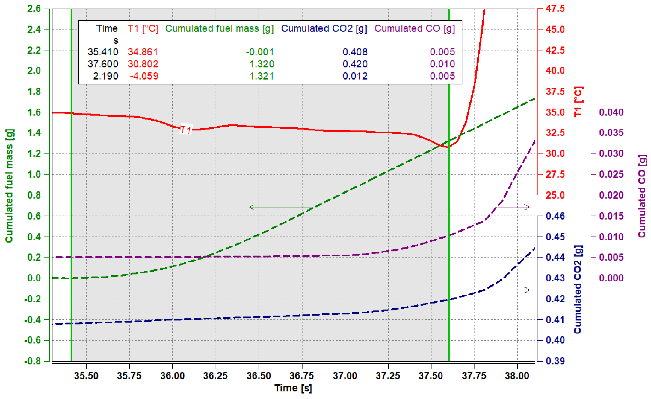
Figure 9 is focused on the period corresponding to the starting delay of the burner: 2.19 s between the moment corresponding to the first positive value of the MFF and the moment when the inlet temperature of the pre-catalytic converter (T1) increases. This period also corresponds to the endothermic phase of the injection, i.e., gasoline absorbs heat for the vaporization, as T1 drops from 34.8 °C to 30.8 °C.
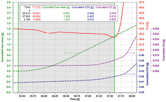
Figure 9.
Starting delay of the burner (see the grey area).
Figure 9 also shows the cumulated values for fuel, CO, and CO2 masses, obtained by integrating their corresponding evolutions in the period of the starting delay of the burner.
Thus, it is about 1.321 g of gasoline injected in this period, which during the events occurring before the start of combustion (SoC) generates 12 mg of CO2 and 5 mg of CO. Regarding the nitric oxides (NO + NO2), a technical problem occurred during the tests and the analyzer was unable to acquire data. However, they should be zero in this phase since the combustion did not start. The presence of CO2 and CO in the exhaust species of the burner during these 2.19 s (regardless of their small amounts) means that some initiations of flames did occur.
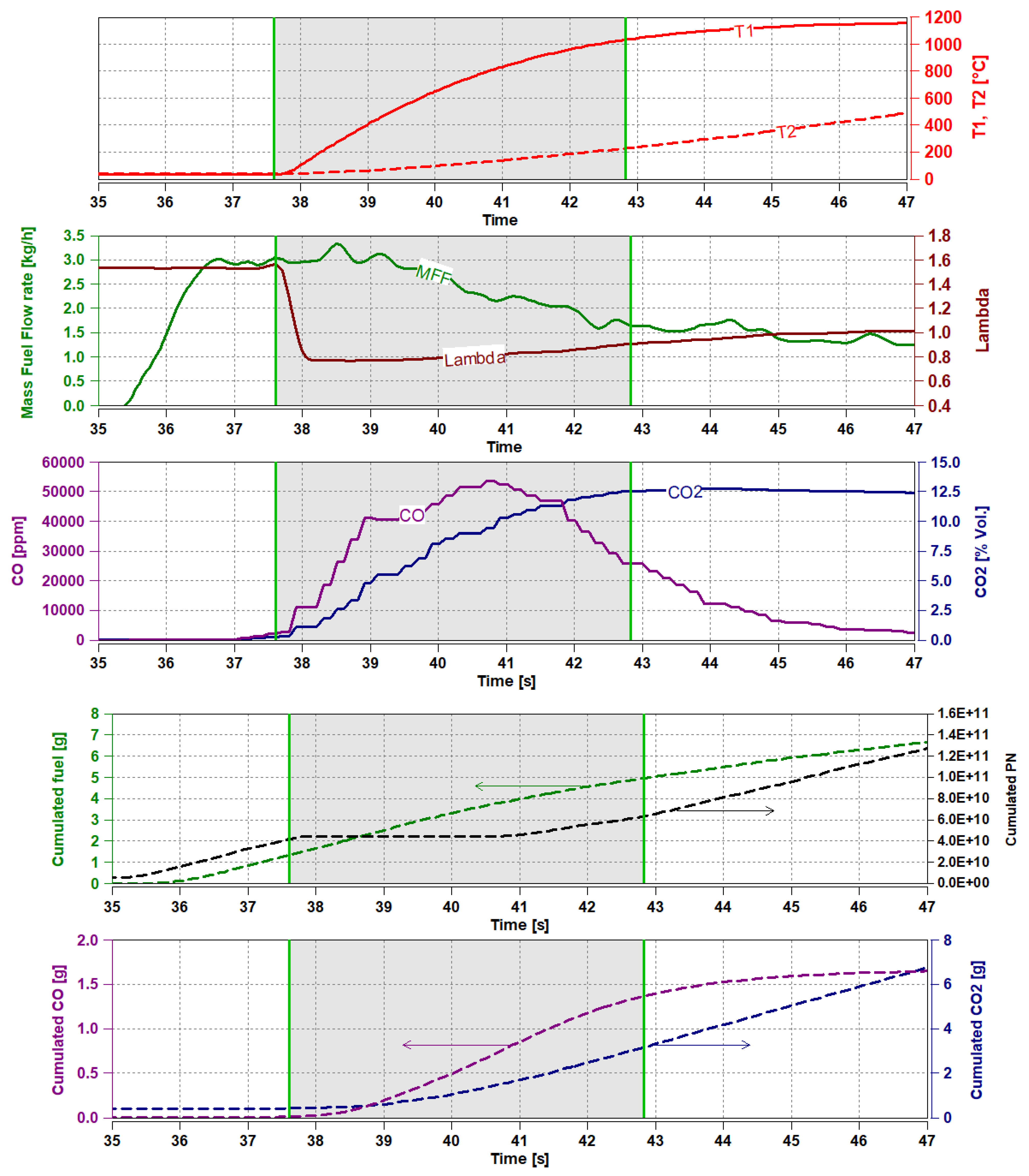
After the starting of the burner (SoB), the focus was on how long it took the pre-catalytic converter to reach the light-off temperature, which in this study was conventionally considered as being 500 K, as discussed in the Introduction section. As seen in Figure 10, T2 (i.e., the temperature in the mid-part of the pre-catalytic converter, Figure 6a) reached this temperature (227 °C) after 5.2 s. At this point, T1 was at 1032 °C and the lambda coefficient arrived at 0.91 (still rich mixture favoring the formation of UHC and CO). According to [26], when not using a burner, i.e., when betting only on the engine to heat up the catalytic converter, with the penalizing measures related to the engine calibration (e.g., increase in the idle speed, lambda-split, spark retardation, as discussed in [13]), it took 21.4 s to reach T2 = 500 K, while the exhaust temperatures measured at the outlet of the cylinder head achieved 700 °C, T1 was at 340 °C, the engine idle speed at this moment was 1306 rpm and the cumulated CO2 during this period was 20.5 g.
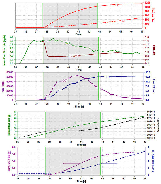
Figure 10.
Experimental results illustrating the TWC light-off period (see the grey area).
Returning to the present analysis, as regards the CO concentration, the same figure shows its instantaneous evolution, as well as the CO2 concentration. By integrating the signals over the light-off period (the grey area illustrated in Figure 10), the following data were obtained: 3.6 g of gasoline injected, which via combustion produced 2.7 g of CO2 and 1.351 g of CO. The lower value of CO2 with respect to the gasoline mass injected and the high mass of CO are an indication of an incomplete combustion occurring in this light-off period, i.e., part of the fuel remaining unburnt. With a UHC gas analyzer, this hypothesis would have been confirmed. The incomplete combustion occurring during the TWC light-off period is also a result of the rich mixtures used (0.78 < lambda < 0.91), as seen in Figure 10. The control system used did not include an automatic regulation of the injection time after T1 started to increase (the sign of SoB or SoC), i.e., automatically adjusting the injection time from the condition to reach lambda 1 or even higher (e.g., 1.2, as seen in [25]), so as to ensure lower CO and UHC. Only to have a measure of comparison, lambda 1 or the stoichiometric mixture is the theoretical condition for complete combustion, meaning that 1 g of octane generates 3.1 g of CO2.
Regarding the air pump, it consumed 360.6 W, while the thermal power of the burner calculated for the complete combustion of the gasoline injected during the light-off period was 12.8 kW (with a specific heat capacity for gasoline of 2.22 kJ/kg/K and a specific heat ratio of 1.35).
On the PN subject, as illustrated in the same figure, before SoB, there are particles (4.1 × 10¹⁰) displaced from upstream the PN counter by the air stream generated by the burner’s air pump. Then, first, there is a stagnation as if there are no more particles generated, followed by an increase in the cumulated PN. In total, the light-off period is characterized by a 2.15 × 10¹⁰ PN. The experimental setup used, Figure 6a, did not include a particulate filter (PF), which nowadays is a standard in the current SI engines for the passenger cars.
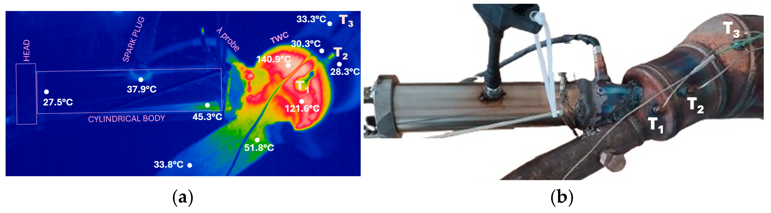
The skin temperatures at 5.2 s after SoB are presented in Figure 11. The slightly higher temperature from the lower part of the burner’s cylindrical body (45.3 °C) could be an indication of a weak combustion occurring inside, in this area, as if some liquid gasoline arriving here was ignited somehow (as seen in Figure 8, the burner was inclined, having the head in a position that is higher than its body outlet, thus favoring the flow of a gasoline film on the lower wall of the cylindrical body). The highest skin temperatures (>100 °C) were in the area where the burner’s flame occurred.
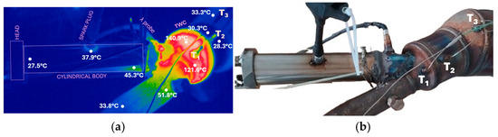
Figure 11.
Skin temperatures at 5.2 s after SoB: (a) picture taken with the thermal camera; (b) real picture of the assembly.
5. Conclusions and Future Works
As previously discussed, the initial question at the origin of this study was to see if a relatively affordable and straightforward extra-combustion device (i.e., a burner) can serve the purpose of reducing the TWC light-off time. The relevance of such a device related to the future development of more ecologic and efficient SIEV was substantiated in this paper with precise data obtained via numerical and experimental investigation, allowing others to replicate and build on the obtained results.
The main findings of this investigation are twofold:
- Based on the CFD study,
- This kind of examination is a good way to decide how to achieve a so-called fit-for-purpose internal aerodynamics of the burner (i.e., to quickly obtain a homogeneous and ignitable mixture) by relying only on a simple design, not using relatively complex elements such as the ones imported from the aeronautical burner application, i.e., relying only on conveniently orienting the two air inlets from the burner’s head;
- Two design improving ideas emerged from this numerical study; however, to be able to draw more pertinent conclusions, all the design iterations should be complemented with CFD studies aiming to see the air–fuel interaction and the combustion process;
- The starting delay of the burner was identified as the parameter to be assessed experimentally to see the effects of the design decisions.
- Based on the experimentation,
- To reach the pre-catalytic converter light-off temperature, conventionally taken as 500 K, the burner was operated at a calculated thermal power of 12.8 kW for 5.2 s and consumed 3.6 g of gasoline, while T1 attained 1032 °C, and the cumulated emissions were: 2.7 g of CO2, 1.351 g of CO and 2.15 × 10¹⁰ particles, respectively;
- To have a comparison measure, when not using a burner, i.e., when betting solely on the engine to heat-up the TWC, with the penalizing measures related to the engine calibration, it took 21.4 s to reach T2 = 500 K, while the exhaust temperatures measured at the outlet of the cylinder head attained 700 °C, T1 was at 340 °C, the engine idle speed at this moment was 1306 rpm and the cumulated CO2 during this period was 20.5 g.
- An enhanced procedure for the burner’s operating control aiming to produce a cleaner combustion during the TWC pre-heating was identified: automatic control of the injection time after SoB from the condition to reach lambda 1 or even higher (if considered suitable).
As for the future works, based on the findings summarized above, another prototype is planned for manufacturing aiming to achieve a lower starting delay of the burner, an improved repeatability of the burner starting and a faster light-off period. Using the burner beyond the TWC pre-heating, i.e., using it in parallel with the engine’s operation when needed (e.g., the operation of the hybridized vehicles, which involves repeating sequences of engine off/on for purely electric drive), is also planned.
Author Contributions
Conceptualization, A.C., B.C. and J.B.; methodology, A.C. and J.B.; data acquisition software and control system, B.C., A.C. and J.B.; CAD and CFD simulation, R.S., A.C. and V.I.-S.; experimental investigation, A.C., B.C., J.B. and R.S.; formal analysis, A.C., R.N. and V.I.-S.; writing—original draft preparation, A.C., B.C. and R.N. All authors have read and agreed to the published version of this manuscript.
Funding
In 2022, this research received funding from our institution gained through the “CIPCS” competition: grant title—“Dezvoltarea unui sistem de amorsare rapidă a convertoarelor catalitice pentru adaptarea autoturismelor la viitoarea normă de depoluare EURO7/Development of a fast TWC light-off system for the adaptation of cars to the future EURO7 norm”.
Data Availability Statement
The raw data supporting the conclusions of this article will be made available by the authors on request.
Acknowledgments
The authors want to thank the following technicians who contributed with the manufacture of the burner prototype: Gheorghe Leașu and Ion Nițescu. We also acknowledge our institution for partially funding our project. Our gratitude goes also to AVL List Gmbh for providing freely the software we used (FIRE and CONCERTO).
Conflicts of Interest
Author Julien Berquez was employed by the company Horse Romania. The remaining authors declare that the re-search was conducted in the absence of any commercial or financial relationships that could be construed as a potential conflict of interest.
Nomenclature
| 2D, 3D | Two, three dimensional |
| AFR | Air–fuel ratio |
| BEVs | Battery Electric Vehicle(s) |
| CFD | Computational Fluid Dynamics |
| CPU | Central Processing Unit |
| CO | Carbon monoxide |
| CO2 | Carbon dioxide |
| DAQ | Data acquisition system |
| EFM | Exhaust flow mass(meter) |
| EHC | Electrically heated catalyst |
| EU | European Union |
| GB | Gigabyte |
| GDI | Gasoline direct injection |
| GHz | Gigahertz |
| HEV | Hybrid electric vehicle(s) |
| HW | Hot wire |
| IC | Internal combustion |
| ICEV | Internal combustion engine vehicle(s) |
| Lambda | Air excess coefficient (AFR made dimensionless by stoichiometric conditions) |
| MAF | Mass air flow(meter) |
| MFF | Mass fuel flow(meter) |
| ms | Milliseconds |
| nm | Nanometers |
| NO | Nitric monoxide |
| NO2 | Nitric dioxide |
| NOx | Nitric oxides (NO + NO2) |
| OSC | Oxygen storage capacity |
| PEMS | Portable Emission Measurement System |
| PF | Particulate Filter |
| PFI | Port-fuel injection |
| PN | Particle number |
| PWM | Pulse Width Modulation |
| RAM | Random access memory |
| RANS | Reynolds-average Navier–Stokes |
| SAE | Society of Automotive Engineers |
| SI | Spark ignition |
| SIEV | Spark ignition engine vehicle(s) |
| SoB | Start of burner |
| SoC | Start of combustion |
| T50, T90 | Temperatures corresponding to a catalyst effectiveness of 50%/90% |
| TKE, k[m2·s−2] | Turbulent kinetic energy |
| TM | Trademark |
| TWC | Three-ways-catalytic converter |
| UHC | Unburnt hydrocarbon |
| USB | Universal Serial Bus |
| ZEVs | Zero-emission vehicle(s) |
| ζ | Eddy viscosity |
| ε | Rate of dissipation |
| f | Relaxation function |
| ɳTWCx | Conversion efficiency or the effectiveness of the catalytic converters for a given pollutant (x) |
References
- Fit for 55. 2024. Available online: https://www.consilium.europa.eu/en/policies/green-deal/fit-for-55/ (accessed on 23 August 2024).
- Fit for 55: Why the EU Is Toughening CO2 Emission Standards for Cars and Vans. 2024. Available online: https://www.consilium.europa.eu/en/infographics/fit-for-55-emissions-cars-and-vans/ (accessed on 23 August 2024).
- Kapus, P. Passenger Car Powertrain 4.x—Fuel Consumption, Emissions and Cost. 2020. Available online: https://www.linkedin.com/pulse/webinar-passenger-car-powertrain-4x-fuel-consumption-emissions-kapus (accessed on 18 July 2024).
- Maurer, R.; Kossioris, T.; Sterlepper, S.; Günther, M.; Pischinger, S. Achieving Zero-Impact Emissions with a Gasoline Passenger Car. Atmosphere 2023, 14, 313. [Google Scholar] [CrossRef]
- Buttes, A.G.D.; Jeanneret, B.; Kéromnès, A.; Le Moyne, L.; Pélissier, S. Energy management strategy to reduce pollutant emissions during the catalyst light-off of parallel hybrid vehicles. Appl. Energy 2020, 266, 114866. [Google Scholar] [CrossRef]
- Sanketi, P.R.; Zavala, J.C.; Hedrick, J.K.; Wilcutts, M.; Kaga, T. A Simplified Catalytic Converter Model for Automotive Coldstart Applications with Adaptive Parameter Fitting. In Proceedings of the the 8th International Symposium on Advanced Vehicle Control, Taipei, Taiwan, 20–24 August 2006. [Google Scholar]
- Shaw, B.T.; Fischer, G.D.; Hedrick, J.K. A simplified coldstart catalyst thermal model to reduce hydrocarbon emissions. IFAC Proc. Vol. 2002, 35, 307–312. [Google Scholar] [CrossRef]
- Zaccardi, J.-M.; Escudie, D. Overview of the main mechanisms triggering low-speed pre-ignition in spark-ignition engines. Int. J. Engine Res. 2014, 16, 152–165. [Google Scholar] [CrossRef]
- Bratan, V.; Vasile, A.; Chesler, P.; Hornoiu, C. Insights into the Redox and Structural Properties of CoOx and MnOx: Fundamental Factors Affecting the Catalytic Performance in the Oxidation Process of VOCs. Catalysts 2022, 12, 1134. [Google Scholar] [CrossRef]
- Gao, J.; Tian, G.; Sorniotti, A.; Karci, A.E.; Di Palo, R. Review of thermal management of catalytic converters to decrease engine emissions during cold start and warm up. Appl. Therm. Eng. 2019, 147, 177–187. [Google Scholar] [CrossRef]
- Steiner, T.; Neurauter, D.; Moewius, P.; Pfeifer, C.; Schallhart, V.; Moeltner, L. Heat-Up Performance of Catalyst Carriers—A Parameter Studyand Thermodynamic Analysis. Energies 2021, 14, 964. [Google Scholar] [CrossRef]
- Langen, P.; Theissen, M.; Mallog, J.; Zielinski, R. Heated Catalytic Converter Competing Technologies to Meet LEV Emissions Standards. SAE J. Fuels Lubr. 1994, 103, 141–150. [Google Scholar]
- Chan, S.H. A practical approach for rapid catalyst light-off by means of strategic engine control. Proc. Inst. Mech. Eng. Part D J. Automob. Eng. 2001, 215, 545–555. [Google Scholar] [CrossRef]
- Real, M.; Hedinger, R.; Pla, B.; Onder, C. Modelling three-way catalytic converter oriented to engine cold-start conditions. Int. J. Engine Res. 2021, 22, 640–651. [Google Scholar] [CrossRef]
- Getsoian, A.B.; Theis, J.R.; Lambert, C.K. Sensitivity of Three-Way Catalyst Light-Off Temperature to Air-Fuel Ratio. Emiss. Control Sci. Technol. 2018, 4, 136–142. [Google Scholar] [CrossRef]
- Samaras, Z.; Hausberger, S.; Mellios, E. Preliminary Findings on Possible Euro7 Emission Limits for LD and HD Vehicles, Brussels. 2020. Available online: https://www.heise.de/downloads/18/3/0/8/5/7/1/4/AGVES-2021-04-08-LDV_Exhaust.pdf (accessed on 10 December 2023).
- Menne, C. Near Zero Impact Pollutant Emissions And Zero CO2—Is There a Future for Combustion Engine Powertrains? Aachen. 2021. Available online: http://siar.ro/wp-content/uploads/2021/05/Christoph-Menne-Near-zero-impact-pollutant-emissions-and-zero-CO2-–-is-there-a-future-for-combustion-engine-powertrains.pdf (accessed on 8 May 2021).
- Barillari, L.; Pipolo, M.; Della Torre, A.; Montenegro, G.; Onorati, A.; Vacca, A.; Chiodi, M.; Kulzer, A. Post-Oxidation Phenomena as a Thermal Management Strategy for Automotive After-Treatment Systems: Assessment by Means of 3D-CFD Virtual Development; SAE Technical Paper; SAE International: Warrendale, PA, USA, 2024; pp. 1–16. [Google Scholar] [CrossRef]
- Kumar, M.; Moriyoshi, Y.; Kuboyama, T. Post-oxidation phenomena enhancement with scavenging and secondary air injection in exhaust manifold of a turbocharged GDI engine. Int. J. Engine Res. 2023, 24, 2388–2409. [Google Scholar] [CrossRef]
- Barillari, L.; Della Torre, A.; Montenegro, G.; Onorati, A.; Rossi, V.; Paltrinieri, S.; Gullino, F. CFD Assessment of an After-Treatment System Equipped with Electrical Heating for the Reduction of the Catalyst Light-Off Time. SAE Int. 2024, 6, 613–627. [Google Scholar] [CrossRef]
- Oser, P.; Mueller, E.; Hartel, G.; Schurfeld, A. Novel Emission Technologies with Emphasis on Catalyst Cold Start Improvements Status Report on VW-Pierburg Burner/Catalyst Systems; SAE Technical Paper 940474; SAE International: Warrendale, PA, USA, 1994; p. 16. [Google Scholar] [CrossRef]
- Kollmann, K.; Abthoff, J.; Zahn, W. Concepts for Ultra Low Emission Vehicles; SAE Technical Paper; SAE International: Warrendale, PA, USA, 1994. [Google Scholar] [CrossRef]
- Della Torre, A.; Barillari, L.; Montenegro, G.; Onorati, A.; Rulli, F.; Paltrinieri, S.; Rossi, V.; Pulvirenti, F. Numerical Assessment of an After-Treatment System Equipped with a Burner to Speed-Up the Light-Off During Engine Cold Start; SAE Technical Paper; SAE International: Warrendale, PA, USA, 2021. [Google Scholar] [CrossRef]
- Montenegro, G.; Torre, A.D.; Barillari, L.; Onorati, A. CFD Investigation of a Burner-base Heating Strategy to Speed up the cold Start Transient of ICEs. In 22. Internationales Stuttgarter Symposium. Proceedings; Springer: Wiesbaden, Germany, 2022. [Google Scholar] [CrossRef]
- Battistoni, M.; Zembi, J.; Casadei, D.; Ricci, F.; Al, E. Burner Development for Light-Off Speed-Up of Aftertreatment Systems in Gasoline SI Engines; SAE Technical Paper 2022-37-0033; SAE International: Warrendale, PA, USA, 2022. [Google Scholar] [CrossRef]
- Clenci, A.; Berquez, J.; Stoica, R.; Niculescu, R.; Cioc, B.; Zaharia, C.; Iorga-Simăn, V. Experimental investigation of the effect of an afterburner on the light-off performance of an exhaust after-treatment system. Energy Rep. 2022, 8, 406–418. [Google Scholar] [CrossRef]
- Hanjalić, K.; Popovac, M.; Hadžiabdić, M. A robust near-wall elliptic-relaxation eddy-viscosity turbulence model for CFD. Int. J. Heat Fluid Flow 2004, 25, 1047–1051. [Google Scholar] [CrossRef]
- Karbon, M.; Sleiti, A.K. Turbulence modeling using Z-F, RSM, LES and WMLES for flow analysis in Z-Shape ducts. In Proceedings of the ASME 2020 Fluids Engineering Division Summer Meeting collocated with the ASME 2020 Heat Transfer Summer Conference and the ASME 2020 18th International Conference on Nanochannels, Microchannels, and Minichannels, Virtual, 13–15 July 2020; p. 3. [Google Scholar] [CrossRef]
- Perceau, M.; Guibert, P.; Clenci, A.; Iorga-Simăn, V.; Niculae, M.; Guilain, S. Investigation of the Aerodynamic Performance of the Miller Cycle from Transparent Engine Experiments and CFD Simulations. Machines 2022, 10, 467. [Google Scholar] [CrossRef]
- Bakker, A. Lectures on Applied CFD. 2008. Available online: https://www.bakker.org/Lectures-Applied-CFD.pdf (accessed on 1 July 2024).

Disclaimer/Publisher’s Note: The statements, opinions and data contained in all publications are solely those of the individual author(s) and contributor(s) and not of MDPI and/or the editor(s). MDPI and/or the editor(s) disclaim responsibility for any injury to people or property resulting from any ideas, methods, instructions or products referred to in the content. |
© 2024 by the authors. Licensee MDPI, Basel, Switzerland. This article is an open access article distributed under the terms and conditions of the Creative Commons Attribution (CC BY) license (https://creativecommons.org/licenses/by/4.0/).