Numerical Study of a Model and Full-Scale Container Ship Sailing in Regular Head Waves

Abstract

In the present study, the added resistance, heave, and pitch of the KRISO Container Ship (KCS) in waves, at both model scale and full scale, are predicted numerically in regular head waves, for four wavelengths and three wave heights. The ISIS-CFD viscous flow solver, implemented in the Fidelity Fine Marine software provided by CADENCE, was employed for the numerical simulations. The spatial discretization was based on the finite volume method using an unstructured grid. The unsteady Reynolds-averaged Navier–Stokes (RANS) equations were solved numerically, with the turbulence modeled by shear stress transport (k-ω) (SST). The free-surface capturing was based on the volume-of-fluid method. The computed solutions were validated through comparisons with towing test data available in the public domain. To predict the uncertainties in the numerical solution, a systematic grid convergence study based on the Richardson extrapolation method was performed for a single wave case on three different grid resolutions. Specific attention was given to the free-surface and wake flow in the propeller plane. The purpose was to compare the numerical results from the model- and full-scale tests to examine the scale’s effect on the ship’s performance in regular head waves. The comparison between the model scale and full scale showed obvious differences, less accentuated for the free-surface topology and clearly observed in terms of boundary layer formation in the propeller’s vicinity.

1. Introduction

The requirements for efficient and sustainable maritime transport are a pressing issue in the face of global climate change. A significant contributor to this challenge is the hydrodynamic performance of ships, which directly impacts their fuel consumption and, consequently, their carbon emissions. Accurate prediction of ships’ hydrodynamic performance is, therefore, a critical aspect of ship design and operation, especially in the context of decarbonization of the shipping industry [1]. This aligns with the global commitment to reduce greenhouse gas emissions and mitigate the impacts of climate change on sustainable development.

Ship hydrodynamic performance is traditionally predicted by extrapolating the model-scale measurements or numerical results to full scale to predict full-scale power requirements [2]. This process involves a series of steps, including data reduction, form factor calculation, blockage corrections, speed correction, and finally, extrapolation using conventional International Towing Tank Conference (ITTC) methods. However, this approach has some limitations and uncertainties due to scaling effects and empirical assumptions. The scale effects resulting from the significant size difference between the model and the full-scale ship, along with the inherent uncertainties in measurements and extrapolation, all contribute to potential inaccuracies in the predicted performance. Furthermore, these procedures primarily address the model scale and often overlook the validation against actual full-scale data, leading to potential discrepancies between the predicted and actual performance of the ship. As such, the accuracy and reliability of full-scale performance prediction remain areas of ongoing research and development in the field of ship hydrodynamics.

Extrapolation procedures are empirical methods to correct the scale effects by applying scaling laws and correction factors to the model-scale data [3,4]. However, these methods are based on assumptions and simplifications that may not be valid for all ship types, speeds, and sea conditions. Moreover, these methods do not account for the nonlinear and viscous effects that are significant at full scale. The scale effect arises due to the discrepancy in force ratios experienced by a model compared to the actual ship. Scale effects arise when the model-scale experiments do not accurately represent the full-scale ship phenomena, due to different Reynolds and Froude numbers, boundary layer thicknesses, flow separation, wave breaking, etc. [5,6]. Therefore, further research and exploration in this area are necessary to improve the accuracy of predictions, to better understand the complex intercorrelations between scale effects and ship hydrodynamics, and to develop methods to account for scale effects. Computational fluid dynamics (CFD) simulations can play a significant role, allowing for more accurate scaling and prediction of full-scale performance.

A review of the existing methods for extrapolating the total resistance has been reported in [2]. The authors approached the problem of predicting full-scale ship performance based on model-scale experiments and scaling laws, which are subject to uncertainties and limitations due to the complex nature of fluid flow and scale effects.

Terziev et al. [5] challenged the assumptions imposed as part of the currently accepted ship resistance extrapolation procedure, which relies on experience-based approaches and large datasets accumulated from years of operation. Their findings suggest that a degree of uncertainty exists in the calculated full-scale resistance, depending on the approach considered. Scale effects on the wave resistance, frictional resistance, and form factor, using different methods and corrections, were extensively investigated. They found that the wave resistance and the free-surface effects on the frictional resistance are not scale-invariant, and that the form factor depends on both the Reynolds and Froude numbers, as also reported in [4]. The authors concluded that the assumption of geometric similarity in ships’ wave patterns and resistance components is not valid, and that a more scientific extrapolation procedure is needed. Based on comparison of towing tank experiments, full-scale CFD simulations, and sea trial measurements for the ship, Niklas and Pruszuko [7] found that the choice of form factor and friction line had a significant influence on the extrapolation of the towing tank results to full scale, leading to variations of up to 19% in the predicted resistance.

The comprehensive study of Bhushan et al. [8] revealed the versatility of a two-point, multilayer wall function model for computing model- and full-scale ship flows with wall roughness and pressure gradient effects. The wall function model was validated for smooth flat-plate flows at Reynolds numbers up to 10⁹, and it was applied to the Athena R/V for resistance, propulsion, seakeeping, and maneuvering simulations. The wall function model showed good agreement with the near-wall turbulence model and experimental data for resistance, propulsion, and boundary layer profiles. The study proved that there is a viable alternative to the near-wall turbulence model for ship hydrodynamics applications, especially for full-scale simulations where the near-wall grid resolution is prohibitive.

Tahsin et al. [9] used a fully nonlinear unsteady RANS CFD method to predict the ship motions and added resistance of a full-scale KCS in regular head waves, at design and slow-steaming speeds. They validated their results against experimental data and estimated the increase in effective power, fuel consumption, and carbon dioxide (CO₂) emissions due to operation in waves. Their study contributes to the literature by providing a comprehensive and detailed analysis of the scale effects in ship hydrodynamics using a state-of-the-art CFD method.

The nominal wake field is important for propeller design and performance, as it affects the efficiency, cavitation, and hull–propeller interaction. However, few studies have focused on how the nominal wake field is influenced by sailing in waves, which is a common situation for most ships. Mikkelsen et al. [10] simulated the KCS at model scale and estimated the ship’s motions and wake field in regular waves with a wavelength equal to the ship length.

The work of Bart Schuiling et al. [11] investigated the scale effect on the prediction of hull pressure fluctuations induced by cavitating propellers. The authors discussed the challenges and limitations of designing and testing non-geosim (geometrically similar) models with prescribed wake characteristics. The scale effect of the nominal wake field of the KCS container ship was investigated by Zhang et al. [12] using the RANS method. Their scope was to solve the viscous flow field of the KCS ship at different scales without considering the free-surface effect. The authors compared the numerical results with experimental data and investigated the relationship between the average axial wake fraction, the Reynolds number, and the propeller radius. The nominal wake characteristics of the KCS at model and full scale were examined by Delen and Bal [13] based on Telfer’s GEOSIM method using CFD. The results showed better accuracy in predicting full-scale performances than other conventional extrapolation methods. The GEOSIM method was found to be more accurate and reliable compared to the 1978 ITTC method for predicting the full-scale effective wake fraction, as it captures the viscous effects in the wake region more accurately [14]. A detailed numerical flow assessment of the boundary layer and wake of a full-scale cargo ship using an IDDES approach was reported in [5].

CFD simulations can predict scale effects in ship hydrodynamics by providing more accurate and detailed representation of the fluid flow in the vicinity of the ship compared to traditional model-scale experiments and extrapolation procedures. CFD simulations can be performed at both model scale and full scale and can consider the nonlinear and viscous effects that are significant, especially at full scale. Therefore, CFD simulations should be used in conjunction with other methods and tools, such as model scale experiments, towing tank tests, and then compared to the full-scale measurements, to obtain a comprehensive and reliable prediction of the ship’s hydrodynamic performance.

This study presents a comprehensive comparison of model- and full-scale ship hydrodynamic flow characteristics, computed using CFD. The disparity between model- and full-scale simulations, primarily due to Reynolds number effects, Froude number effects, and scale effects on roughness, often leads to discrepancies in predicting the actual performance of the ship. Taking advantage of the CFD capabilities, this study aims to bridge this gap, providing a deeper understanding of the flow phenomena around the ship hull under various conditions. The findings of this research have important implications towards the design and operation of more efficient and sustainable ships, contributing to the broader goal of decarbonization in the shipping industry.

The KRISO (Korea Research Institute of Ships and Ocean Engineering) Container Ship (KCS) is the subject of the present study. In order to determine the wave added resistance, the first set of simulations are performed in calm water conditions. In the case of regular head wave simulations, several cases are analyzed comprising four wavelengths, including short and long waves, and three wave heights, for both calm water and regular head wave conditions. The ship speed is set to the design speed corresponding to a Froude number value of 0.261. A total number of twenty-eight simulation cases are performed and reported, following the proposed cases in the Tokyo 2015 Workshop on CFD in Ship Hydrodynamics. The objective is to estimate the wave added resistance, heave, and pitch motions in regular head waves. Also, the comparison between model and full scale for free-surface and wake flow in the propeller plane is investigated in order to understand the scale effect on the ship’s performance in calm water and specifically in waves. The numerical results are validated using the experimental data provided in the Tokyo 2015 Workshop. To evaluate the numerical errors, a verification study was conducted based on a grid and time step convergence test.

2. Numerical Approach

The numerical simulations are performed utilizing the ISIS-CFD solver, developed by the EMN (Equipe Modélisation Numérique) and implemented in Fidelity Fine Marine software version 11.1. This solver employs the finite volume method, a numerical technique used for the spatial discretization of transport equations [15]. The primary purpose of this method is to solve the incompressible unsteady Reynolds-Averaged Navier–Stokes (RANS) equations.

The Unsteady Reynolds-Averaged Navier–Stokes (URANS) equations are equations of motion for fluid flow that are time-averaged to model turbulence. The principle behind these equations is the Reynolds decomposition, where an instantaneous quantity is broken down into its time-averaged and fluctuating quantities.

For a stationary flow subjected to external forces, the time-averaged continuity and momentum equations can be expressed in a Cartesian coordinate system as follows:

$$\frac{\partial \left(\rho {\overline{u}}_i\right)}{\partial x_i}=0$$

(1)

$$\frac{\partial \left(\rho {\overline{u}}_i\right)}{\partial t}+\frac{\partial }{\partial x_j}\left(\rho {\overline{u}}_i{\overline{u}}_j+\rho \overline{u_i^{\prime }{u}_j^{\prime }}\right)=-\frac{\partial \overline{p}}{\partial x_i}+\frac{\partial {\overline{\tau }}_{ij}}{\partial x_j}$$

(2)

where $\rho$ denotes density, $u_i$ represents the vector of relative averaged velocity between the fluid and the control volume, $u_i^{\prime }{u}_j^{\prime }$ signifies the Reynolds stresses, $p$ represents the mean pressure, and ${\tau }_{ij}$ is the mean viscous stress tensor component for a Newtonian fluid under the assumption of incompressible flow, and it can be written as:

$${\overline{\tau }}_{ij}=\mu \left(\frac{\partial {\overline{u}}_i}{\partial x_j}+\frac{\partial {\overline{u}}_j}{\partial x_i}\right)$$

(3)

where $\mu$ is the dynamic viscosity.

Turbulence closure, a critical aspect of fluid dynamics simulations, is accomplished using the k-ω Shear Stress Transport (SST) model [16]. This model employs a near-wall resolution based on a wall function, which is a strategy to manage the computational complexity near the wall in turbulent flow simulations.

The construction of unstructured meshes, which are flexible and efficient for complex geometries, is facilitated by a generalized three-dimensional face-based method. This method allows for the creation of meshes that can adapt to the geometry of the problem, improving the accuracy of the solution.

The coupling of velocity and pressure, two fundamental quantities in fluid dynamics, is achieved using the Semi-Implicit Method for Pressure-Linked Equations (SIMPLE) [17]. In this approach, the velocity field is derived from the momentum conservation equations, while the pressure field is extracted from the mass conservation constraint, also known as the continuity equation [18]. This constraint is then transformed into a pressure equation.

The simulation of free-surface flow, which is the flow with a free surface at its boundary such as the waterair interface, is conducted using a multi-phase flow approach. This approach is based on the volume-of-fluid (VOF) method, a popular method for capturing the free surface in computational fluid dynamics.

The modeling of incompressible and non-miscible flow phases, where the fluids do not mix and maintain a constant density, is performed using conservation equations for each volume fraction of phase/fluid [19]. This approach ensures the accurate representation of each phase or fluid in the flow.

The convection and diffusion terms in the RANS equations, which represent the transport of quantities due to bulk fluid motion and random molecular motion, respectively, are discretized using a second-order upwind scheme and a central difference scheme. These schemes provide a balance between accuracy and computational efficiency.

For time discretization, an implicit scheme is applied. This type of scheme offers stability for larger time steps, making it suitable for unsteady computations. Furthermore, a second-order three-level time scheme is employed for time-accurate unsteady computation, ensuring the accuracy of the solution in time-dependent problems [20].

3. Computational Strategy

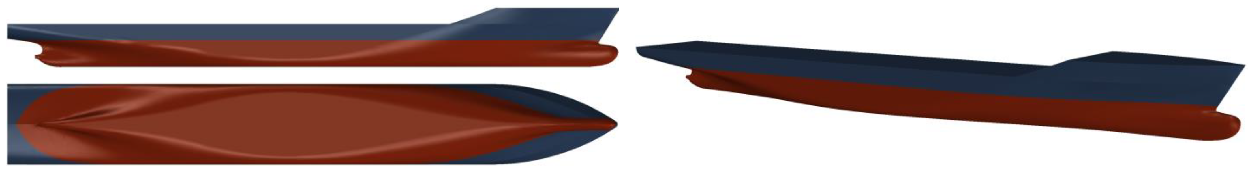
3.1. Ship Geometry

The KRISO Container Ship (KCS) is a contemporary container vessel, designed to study the fluid dynamics around a ship, featuring a bulbous bow and a transom stern. It was first introduced as a benchmark at the Gothenburg workshop in 2000, in order to evaluate the accuracy of Computational Fluid Dynamics (CFD) techniques. The Korea Research Institute of Ships and Ocean Engineering (KRISO) conducted towing tank experiments to gather data on resistance, flow patterns around the hull, and the free surface [21,22,23]. Also, the National Maritime Research Institute (NMRI) conducted extensive research and tests to determine the heave and pitch motion and wave added resistance in regular head waves [24]. The ship’s geometry and main dimensions are depicted in Figure 1 and

Table 1. Main particulars.

Main Particulars	Symbol	Model Scale	Full Scale
Length between perpendiculars	$L_{PP} \left[\mathrm{m}\right]$	6.0702	230.0
Length of waterline	$L_{WL} \left[\mathrm{m}\right]$	6.1357	232.5
Maximum beam of waterline	$B_{WL} \left[\mathrm{m}\right]$	0.8498	32.3
Draft	$T \left[\mathrm{m}\right]$	0.2850	10.8
Displacement volume	$\nabla \left[{\mathrm{m}}^3\right]$	0.9571	53,030
Block coefficient	$C_B \left[-\right]$	0.6505	0.6505
Wetted surface area	$S_W \left[{\mathrm{m}}^2\right]$	6.6978	9539

, respectively.

3.2. Test Cases

The study includes two categories of simulation; the first is dedicated to the ship analysis in calm water, which is established as a base for the second simulation that investigates the ship performance in regular head waves. Both categories include analysis of the ship in model and full scale. In the calm water simulation, the ship resistance is measured and recorded to compare the resistance values that will be obtained in waves to extract the added wave resistance. Ship speed is set to the design speed corresponding to a Froude number ($Fr$) value of 0.261. The regular wave parameters are selected such that the wavelength ($\lambda$) is set to four different values, including short and long waves, while the wave height is set to three wave heights ($H_w$). The test case summary is tabulated in

Table 2. Test cases.

$\mathit{F}\mathit{r}$	$\mathit{\lambda }/{\mathit{L}}_{\mathit{p}\mathit{p}}$	${\mathit{\lambda }}_{\mathit{m}\mathit{o}\mathit{d}\mathit{e}\mathit{l} \mathit{s}\mathit{c}\mathit{a}\mathit{l}\mathit{e}} \left[\mathbf{m}\right]$	${\mathit{\lambda }}_{\mathit{f}\mathit{u}\mathit{l}\mathit{l}-\mathit{s}\mathit{c}\mathit{a}\mathit{l}\mathit{e}} \left[\mathbf{m}\right]$	${\mathit{H}}_{\mathit{w}}/{\mathit{L}}_{\mathit{p}\mathit{p}}$	${\mathit{H}}_{\mathit{w} \mathit{m}\mathit{o}\mathit{d}\mathit{e}\mathit{l} \mathit{s}\mathit{c}\mathit{a}\mathit{l}\mathit{e}} \left[\mathbf{m}\right]$	${\mathit{H}}_{\mathit{w} \mathit{f}\mathit{u}\mathit{l}\mathit{l}-\mathit{s}\mathit{c}\mathit{a}\mathit{l}\mathit{e}} \left[\mathbf{m}\right]$
0.261	0.000	0.000	0.000	0.000	0.000	0.000
	0.651	3.949	149.628	0.010	0.063	2.349
				0.020	0.123	4.660
				0.032	0.196	7.426
	0.851	5.164	195.664	0.010	0.063	2.349
				0.013	0.078	2.955
				0.020	0.123	4.660
				0.032	0.196	7.426
	1.150	6.979	264.434	0.010	0.063	2.349
				0.020	0.123	4.660
				0.032	0.196	7.426
	1.951	11.840	448.618	0.010	0.063	2.349
				0.020	0.123	4.660
				0.032	0.196	7.426

, showing the wave parameters as nondimensional values with respect to the ship length. These test cases are intentionally selected to match the ones proposed in the Tokyo Workshop on CFD in ship Hydrodynamics [25,26] for validation purposes. The total number of simulation cases performed in this study is twenty-eight.

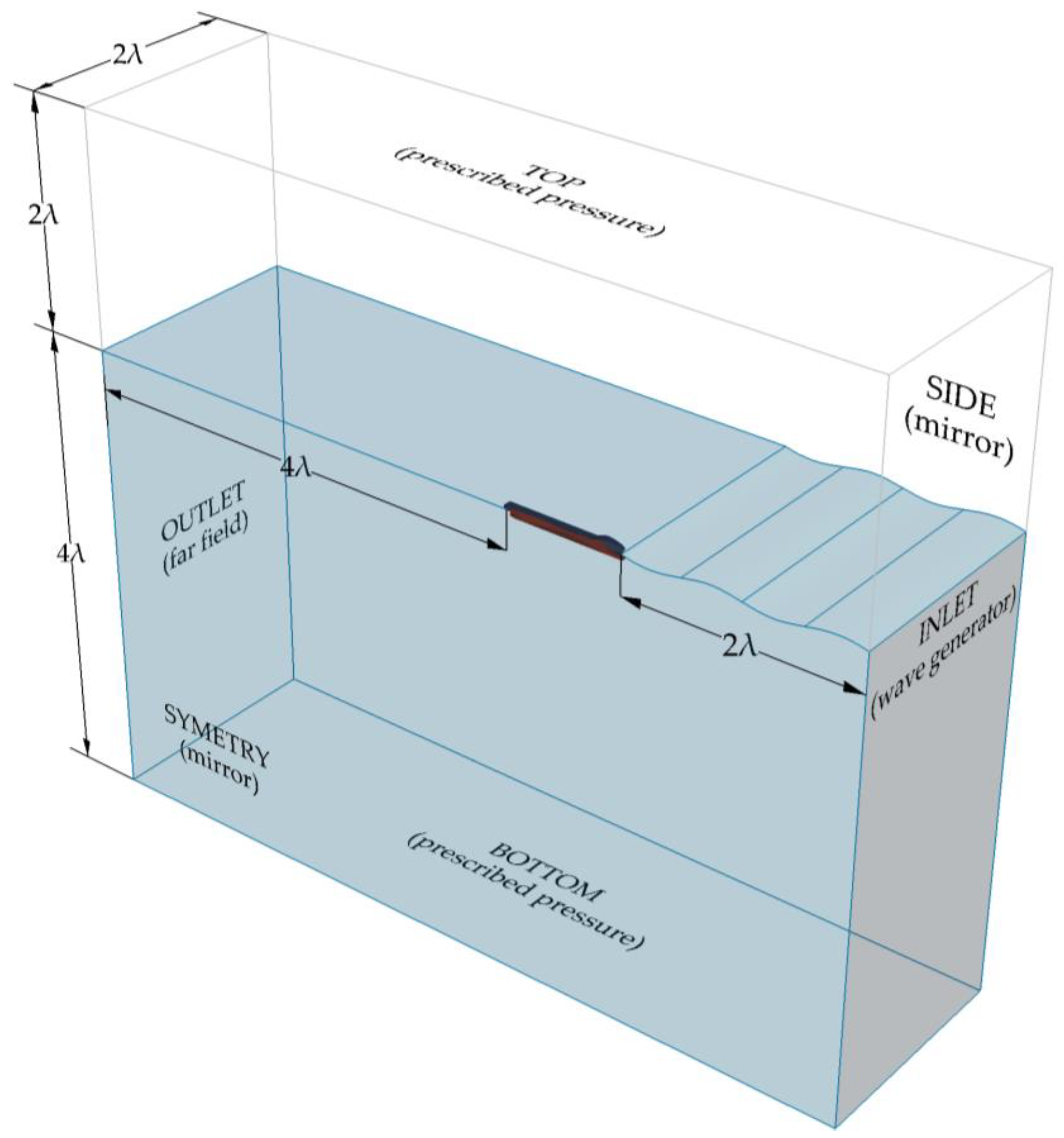
3.3. Computational Domain

The computational domain for all performed simulations in this study is configured as a prism with a rectangular section. Since the simulations include only calm water and head waves, the symmetry condition is imposed on the centerline of the ship plane in order to reduce the computational effort and simulation time. The origin of the coordinate system is set at the intersection between the aft perpendicular and the design waterline, which is set to the draft corresponding values, as represented in Table 1 for both model and full scale. This sets the undisturbed free-surface position at z = 0, which makes it easier to analyze the output data after simulation. The domain’s dimensions and boundary conditions are selected to comply with the ITTC recommendations [27].

As depicted in Figure 2, the dimensions of the computational domain are set as a function of wavelength $\lambda$, such that the inlet is located at $2.0\lambda$ in the upstream from the forward perpendicular, and the outlet is positioned at $4.0\lambda$ downstream from the aft perpendicular in $x$-axis direction. In the $y$-axis direction, the side boundary is situated $2.0\lambda$ from the center line of the ship, and the symmetry plane aligns with the ship’s central line at y = 0. Finally, for the $z$-axis direction, the top boundary is set at $2.0\lambda$ above the undisturbed free-surface level, while the bottom is positioned at $4.0\lambda$ below.

Regarding the boundary conditions, the symmetry plane is defined as a mirror. The inlet boundary serves as a wave generator, where an interface equation is added to the governing equations based on the interface parameter c. This parameter is linked to the regular wave generator equation, ${\zeta }_{\left(x,t\right)}={\zeta }_a\sin \left(kx-\omega t+\epsilon \right)$, where k is the wave number, ω is the wave angular frequency, and ε stands for the phase shift. The volume fraction parameter c follows the interface through this equation, whereas c = 0 in the air, c = 1 in the water, and finally, the interface captures the water surface when c = 0.5, corresponding to the wave elevation equation. The outlet boundary is considered far field. The side boundary is also defined as a mirror to prevent wave reflection phenomena, while the top and bottom boundaries are defined as prescribed pressure. For the ship’s hull, a wall-function condition is adopted with $y^{+}=50$ for the model scale and $y^{+}=300$ for the full scale, while the ship’s deck is set to slip condition, because it is assumed to remain in the air during the simulation, where the viscous effect in air compared to that in water can be ignored. At the free-surface level, the downstream zone is set to provide sufficient length for wave damping to avoid reflection from the downstream boundary. This zone has four times the wavelength divided as follows. One wavelength is dedicated to the free-surface prediction, another wavelength is chosen as a damping relaxation zone with a slightly larger grid size, and, finally, the last two wavelengths have a large grid size at the free-surface level to provide a sufficient numerical wave damper.

3.4. Computational Grid and Grid Convergence Test

The computational grids for all test cases are the unstructured hexahedral type. They are adapted to be suitable for those four wavelengths and three wave heights considered for this investigation. As shown in Figure 3, the refinement around stern and bow areas is increased to capture the wake in the propeller plane using an isotropic refinement cylinder.

Regarding the free surface, two rectangular boxes are used to refine the entire computational domain. The first box starts upstream and extends for one wavelength downstream of the ship’s hull. The cell size in this box is chosen to provide 60 cells/wavelength in x- and y-directions, which is considered sufficient, as recommended by ITTC and other researchers; in particular, the ship is considered within the medium-high speed category, which makes it easier to capture the free surface compared to slower ships. In the vertical direction, the refinement boxes extend over three times the wave height, evenly distributed above and below the undisturbed free surface. The refinement criteria in that direction are selected to provide 16 cells per wave height, as recommended by the program user manual, which was shown to be sufficient by other researchers, such as the work reported in [28]. The second box extends for the entire three wavelengths downstream and serves as a numerical damping zone. The refinement criteria in the z-direction are maintained unchanged, while the cell size in x- and y-directions is increased gradually until it reaches 8 times the value in the refinement box, which means that the cell size in that zone provides only 8 cells per wavelength. It is worth mentioning that because the simulation has several wavelengths and wave heights, it was important to establish the refinement criteria to be sufficient for all cases. For this reason, the refinement zone dimensions are selected based on the longest and highest wave in the simulation cases, to provide sufficient refinement areas. On the other hand, the cell size in x-, y-, and z-directions was chosen based on the smallest wavelength and height, to ensure sufficient refinement even for the smallest wave parameters.

To assess the numerical errors and uncertainties of the simulations, a grid convergence test is conducted for both model scale and full scale, based on the Richardson extrapolation method reported in [29]. For each ship scale, three computational grids with different refinement levels are generated with an average refinement ratio $r_G=\sqrt{2}$. Thus, the coarse grid (Figure 3a) counted approximately 9.1 million cells for the model scale and 9.3 million cells for the full scale, the medium grid (Figure 3b) has 12.9 million cells for the model scale and 13.2 million cells for the full scale, and, finally, the fine grid (Figure 3c) has approximately 18.2 million cells for the model scale and 18.6 million cells for the full scale.

It is worth mentioning that the time-step convergence test details in this study, though it was performed, were omitted, since the comparison showed that it has no effect on the numerically obtained results. The time step was chosen to provide 600 iterations per wave period, which is 4 times larger than the ITTC recommendations for seakeeping simulation. This value has proven to be sufficient for seakeeping simulations using the same CFD code, as reported in [28].

Table 3. Grid convergence test results.

Scale	Parameter	${\mathit{\epsilon }}_{21}$	${\mathit{\epsilon }}_{32}$	${\mathit{R}}_{\mathit{G}}$	${\mathit{\delta }}_{\mathit{G}}$	${\mathit{U}}_{\mathit{G}}$
MODEL-SCALE	$R_{T_W}$	6.394	11.023	0.580	8.832	8.832
	$R_{T_W} Amp.$	6.118	9.966	0.614	9.727	9.727
	$z Amp.$	−0.008	−0.012	0.689	−0.018	0.018
	$\theta Amp.$	−0.002	−0.003	0.593	−0.003	0.003
FULL-SCALE	$R_{T_W}$	4.529	7.113	0.637	7.935	7.935
	$R_{T_W} Amp.$	7.779	17.827	0.525	8.584	8.584
	$z Amp.$	−0.008	−0.017	0.458	−0.007	0.009
	$\theta Amp.$	−0.002	−0.008	0.227	−0.001	0.003

contains the grid convergence test results for the total resistance in wave $\left(R_{T_W}\right)$ and its amplitude ($R_{T_W} Amp.$), and also for heave amplitude ($z Amp.$) and pitch amplitude ($\theta Amp.$), for both model scale and full scale.

The convergence ratio, $R_G$, was calculated as follows:

$$R_G=\frac{{\epsilon }_{i,21}}{{\epsilon }_{i,32}}$$

(4)

Here, ${\epsilon }_{i,21}$ and ${\epsilon }_{i,32}$ represent the simulation error, determined by:

$${\epsilon }_{i,21}=S_{i,2}-S_{i,1};{\epsilon }_{i,32}=S_{i,3}-S_{i,2}$$

(5)

where $S_{i,1}$, $S_{i,2}$, and $S_{i,3}$ are the solutions obtained from numerical calculations.

If the convergence ratio is within the range $0<R_G<1$, then the computational grid is monotonically convergent. In the case of $R_G<0$, it indicates oscillatory convergence, and if $R_G>1$, it is considered divergent.

To calculate the accuracy error, ${\delta }_G$, the following expression is used:

$${\delta }_G=\frac{{\epsilon }_{i,21}}{r_G^{p_G}-1}$$

(6)

where $p_G$ is the accuracy level determined by:

$$p_G=\frac{\ln \left({\epsilon }_{i,32}/{\epsilon }_{i,21}\right)}{\ln \left(r_G\right)}$$

(7)

The numerical uncertainty is determined with the expression:

$$U_G=\left|C_G·{\delta }_G\right|+\left|\left(1-C_G\right)·{\delta }_G\right|$$

(8)

Here, $C_G$ is the correction factor calculated with:

$$C_G=\frac{r_G^{p_G}-1}{r_G^{p_{th}}-1}$$

(9)

where $p_{th}$ is the theoretical accuracy level, considered as $p_{th}=2$.

For both scale cases, the fine grid was used further for numerical simulation in order to capture a better resolution of the flow around the ship’s hull and the wake in the propeller plane.

3.5. Simulation Setup

The calm water simulation is performed using a quasi-static approach with only two degrees of freedom taken into consideration, referring to sinkage and trim. The time step is selected corresponding to the ITTC recommended practice for ship resistance CFD simulations [27], such that the time step is decided based on the formula $\Delta t=0.005L_{PP}/U$, where $L_{pp}$ stands for the ship length, while $U$ refers to the ship speed. The simulation setup includes eight nonlinear iterations with second-order convergence criteria using a combined central and upwind differencing scheme. The simulation is performed until the convergence of forces and vertical motion is achieved, which refers to a condition when the change in solution is less than or equal to 1% of the obtained value.

The head wave simulation is fully unsteady and also has only two degrees of freedom considered, referring to heave and pitch motions. The ship is sailing at the design speed in the corresponding simulation case parameters regarding wavelength and height in two-phase flow. The simulation setup included twelve nonlinear iterations with fourth-order convergence criteria using a combined central and upwind differencing scheme. The simulation is performed until the ship encounters at least 15 waves. It is important to mention here that the encounter milestone starts once the wave crest interacts with the forward perpendicular of the ship; this by default is considered as moment zero with respect to the program simulation. This instance will be used while presenting the results as $t/Te=0.00$, while the moment when the trough aligns with the forward perpendicular is referred to as $t/Te=0.50$; the other two instances are denoted by $t/Te=0.25$ and $t/Te=0.75$, referring to the instance when that wave aligns with the forward perpendicular at the mid-span between crest and trough for the first and between the trough and crest for the latter.

4. Results and Discussions

To make it easier to follow the results within this study, the results are initially validated to confirm that the numerical approach is sufficiently accurate, then the comparison between model- and full-scale ship simulations are presented later.

4.1. Verification and Validation

For validation purposes, the following sub-sections provide direct comparison between the experimental fluid dynamics (EFD) data retrieved from the Tokyo Workshop [25,26] and the obtained CFD results in this study. The results considered in this comparison are the total resistance coefficient in calm water $C_{T_C}$,vertical translation in the z-direction (sinkage) z, and finally, the rotation around the y-axis (trim) θ.

As for the head wave simulation, the comparison is performed in terms of total resistance in wave coefficient $C_{T_w}$ and nondimensionalized motion response in the vertical plane (heave $z/{\zeta }_s$ and pitch: $\theta /k{\zeta }_s$), where ${\zeta }_s$ refers to wave amplitude, while k refers to wave number and can be calculated as a function of wavelength $\lambda$ such that $k=2\pi /\lambda$.

4.1.1. Calm Water Conditions

Comparing the result obtained in calm water conditions through numerical simulation with the experimental data,

Table 4. Relative difference between CFD and EFD in calm water conditions.

$\mathit{F}\mathit{r}$	$\mathit{v} \left[\mathbf{m}/\mathbf{s}\right]$	${\mathit{C}}_{{\mathit{T}}_{\mathit{C}}}$	$\mathit{z}$	$\mathit{\theta }$
0.261	2.017	−1.22%	−6.88%	3.96%

presents the relative difference between the CFD results and EFD data. As the results bear out, the total resistance in calm water is underpredicted by 1.22% compared with towing tank results. In terms of ship motions, sinkage is underpredicted, with 6.88%, and trim is overpredicted, with 3.96%, compared to the EFD data. This shows that the simulation is accurate in terms of predicting ship resistance especially, and acceptable in terms of ship motions.

4.1.2. Head Wave Conditions

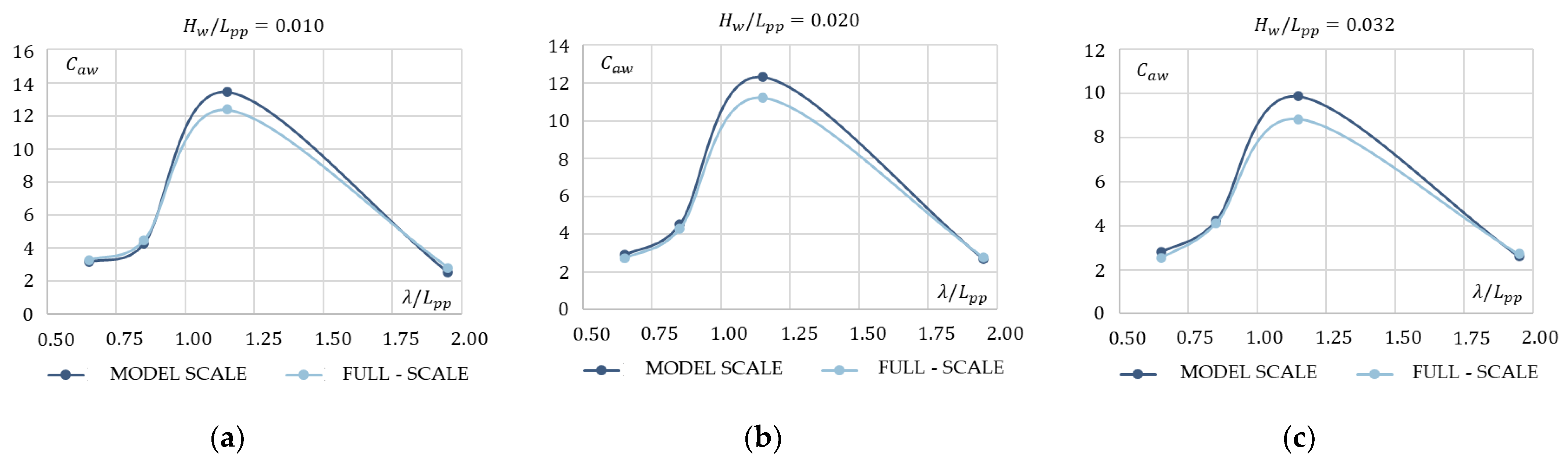
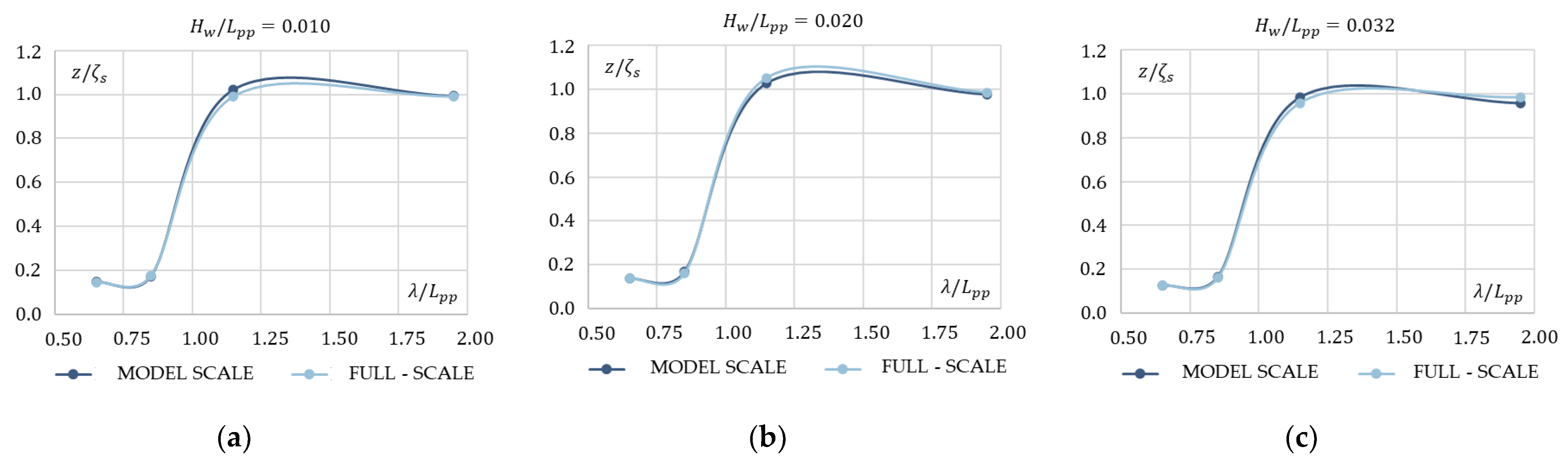
Next, a set of simulations are performed in head wave conditions for the model scale.

Table 5. Relative difference between CFD and EFD in regular head wave conditions.

$\mathit{\lambda }/{\mathit{L}}_{\mathit{p}\mathit{p}}$	${\mathit{H}}_{\mathit{w}}/{\mathit{L}}_{\mathit{p}\mathit{p}}$	${\mathit{C}}_{{\mathit{T}}_{\mathit{W}}}$	$\mathit{z}/{\mathit{\zeta }}_{\mathit{s}}$	$\mathit{\theta }/\mathit{k}{\mathit{\zeta }}_{\mathit{s}}$
0.651	0.010	−1.87%	14.42%	34.51%
0.851	0.013	−4.56%	−29.11%	33.81%
1.150	0.020	9.95%	14.37%	−3.61%
1.951	0.032	9.32%	2.74%	10.88%

contains the relative difference between CFD and EFD results for the total resistance coefficient in waves ($C_{T_W})$, heave ($z/{\zeta }_s$), and pitch ($\theta /k{\zeta }_s$) amplitude. The “$w$” index represents the regular head wave conditions. Figure 4 displays the comparison between CFD and EFD curves for total resistance coefficient in waves, heave, and pitch amplitudes. The absolute average relative difference for the resistance coefficient in waves is 6.4%, while for the motions’ amplitudes, the values are 15.2% for heave and 20.7% for pitch. The motion amplitudes have a considerably significant difference compared to the EFD data, yet it is less than 10% for ship resistance, which has significant weight in this study. On the other hand, despite the difference in the numerically obtained results, the technique remains the same in the present comparison for model and full scale, which makes the comparison solid from this perspective. The main reason behind these differences may be due to the grid quality, which means that a finer grid could enhance the obtained results. Nevertheless, this comes with a significant simulation cost. Another reason may be related to the over- or under-estimation of the numerical damping, since both motions are mainly affected by the motion damping criteria.

The comparison between CFD and EFD in terms of total resistance coefficient in waves and nondimensionalized vertical motions is brought to the reader’s attention in Figure 5 for the case study when $\lambda /L_{pp}=0.651$ and $H_w/L_{pp}=0.010$. The results also confirm the previous discussion regarding the accuracy of simulation for total resistance coefficient and the difference for the predicted motions.

In an extended context, the comparison between CFD and EFD in terms of total resistance coefficient in waves and nondimensionalized vertical motions is brought to the reader’s attention in Figure 6 for the case study when $\lambda /L_{pp}=0.851$ and $H_w/L_{pp}=0.013$. The results have better resemblance for total ship resistance coefficient and vertical motions in waves.

Furthermore, the comparison between CFD and EFD in terms of total resistance coefficient in waves and nondimensionalized vertical motions is brought to the reader’s attention in Figure 7 for the case study when $\lambda /L_{pp}=1.150$ and $H_w/L_{pp}=0.020$. The results have better resemblance for total ship resistance coefficient and vertical motions in waves. It is worth mentioning that in Figure 7a, the total resistance coefficient was only provided as a medium value, not a time series.

Finally, the comparison between CFD and EFD in terms of total resistance coefficient in waves and nondimensionalized vertical motions is brought to the reader’s attention in Figure 8 for the case study when $\lambda /L_{pp}=1.150$ and $H_w/L_{pp}=0.020$. Here, the accuracy of the numerically predicted results is significantly improved.

Concluding the previously described validation process, it can be observed that the results for calm water are sufficiently accurate in terms of resistance and vertical motion. The cases of the ship sailing in waves revealed that the accuracy of the obtained results is relatively acceptable in terms of ship resistance coefficient in waves, and less accurate for vertical motions in waves, especially for the small wavelength and wave height. The accuracy of the obtained results improves as the wavelength and wave height increase. For this reason and to maintain a logical comparison between model scale and full scale while taking into consideration the free surface and wake flow, the final case with the maximum wavelength and wave height will be discussed in Section 4.2.

4.2. Scale Effect

In order to determine the added resistance in waves, total resistance in calm water must be determined. Thus, also for the full scale, the first step was to determine the total resistance in calm water.

The wave added resistance coefficient is calculated with the following expression:

$$C_{AW}=\frac{R_{T_w}-R_{T_c}}{\rho ·g·{\left(H_w/2\right)}^2·B_{WL}^2/L_{pp}}=\frac{R_{AW}}{\rho ·g·{\left(H_w/2\right)}^2·B_{WL}^2/L_{pp}}$$

(10)

where $R_{T_w}$ is the total resistance in waves and $R_{T_c}$ is the total resistance in calm water, $\rho$ represents the water density, $g$ represents gravitational accelerations, $H_w$ is the wave height, $B_{WL}$ represents the beam of the waterline, and $L_{pp}$ is the length between perpendiculars.

Table 6. Relative difference between model scale and full scale in regular head wave conditions.

$\mathit{\lambda }/{\mathit{L}}_{\mathit{p}\mathit{p}}$	${\mathit{H}}_{\mathit{w}}/{\mathit{L}}_{\mathit{p}\mathit{p}}$	${\mathit{C}}_{\mathit{A}\mathit{W}}$	$\mathit{z}/{\mathit{\zeta }}_{\mathit{s}}$	$\mathit{\theta }/\mathit{k}{\mathit{\zeta }}_{\mathit{s}}$
0.651	0.010	3.37%	−1.09%	−10.59%
	0.020	−6.70%	1.24%	5.57%
	0.032	−9.29%	1.34%	−2.10%
0.851	0.010	4.17%	1.89%	−1.73%
	0.020	−5.38%	−4.14%	−3.24%
	0.032	−2.66%	−3.11%	−5.92%
1.150	0.010	−7.81%	−3.08%	−6.83%
	0.020	−9.07%	2.32%	−5.69%
	0.032	−10.61%	−2.66%	−8.42%
1.951	0.010	11.20%	−0.23%	−0.20%
	0.020	2.78%	0.84%	0.98%
	0.032	4.36%	2.74%	2.79%

represents the quantitative relative difference between model- and full-scale results numerically obtained in regular head waves. The results include the added resistance in wave coefficient C_AW, and nondimensional heave and pitch amplitudes, as previously explained. The schematic diagram for the added wave resistance coefficient is plotted in Figure 9 for model- and full-scale ships as a function of the nondimensionalized wavelength at different wave heights.

Similarly, the nondimensionalized vertical motions (heave and pitch) are depicted for model and full scale in Figure 10 and Figure 11 as a function of the nondimensionalized wavelength at different wave heights.

In Figure 12, the comparisons between model scale and full scale are presented for wave profile in calm water condition. It can be observed that the relative wave height generated by the hull is more significant in the full scale compared to the model scale, especially in the stern zone and the downstream, although the wave configurations are almost identical. This may be related to the significant difference in size, which may result in a pressure change at the stern shoulders; this was also observed in other research papers, as reported in [30,31].

Comparing the wave resistance coefficients, a difference of 8.1% is observed between model- and full-scale calculation at a Froude number of 0.261. Even if the differences in wave resistance coefficient between scale factors could be subjective due to numerical errors, a change in wave resistance coefficient implies a geometrically non-similar wave pattern between scale factors [2], which is also sustained by the wave elevation comparison presented in Figure 12.

The comparison between the model- and full-scale free-surface profiles at $\lambda /L_{pp}=1.951$ and $H_w/L_{pp}=0.032$ (which is the case study with the maximum wavelength and height) is brought to the reader’s attention in Figure 13 at the previously described four encountering instances of the wave with the forward perpendicular. The same observation for calm water persists, where the free surface is more accentuated in the full scale compared to the model scale. It can also be observed that there is a slight phase shift at the predicted wave profile.

To investigate the occurrence of the green water on the deck, the mass fraction comparison between model and full scale at $\lambda /L_{pp}=1.951$ and $H_w/L_{pp}=0.032$ is depicted in Figure 14 at the same four encountering instances. The results indicate that the green water phenomenon takes place as soon as the trough leaves the forward perpendicular and heads downstream. In this condition, the pitch motion is reaching a trough value, which tends to push the ship bow downwards, causing the water to overflood the forecastle even with the high forward shear at the bow. This poses a possible hazard for marine operations during similar or extremer sailing conditions and should be taken into consideration to avoid this problem by means of bulwark or higher shear value for the ship’s forecastle.

To gain an insight into the nominal wake field distribution, the nominal wake contours at the propeller plane for the ship sailing in calm water and regular head waves at different wave instants are provided in Figure 15 for both model and full scale. A general tendency of higher axial velocities on the two sides of the propeller hub and lower axial velocities above and especially below the propeller hub are observed for all cases, model and full scale, as was also observed in [10]. Moreover, the Reynolds number increases, the gradient of the wake change decreases slightly, and the wake field at the propeller disk becomes more uniform, which was also confirmed by the study reported in [12]. In the calm water case, the difference between the wake flow contours in the propeller plane can be observed. The model scale reveals the presence of two contrarotating central vortices and the contours are basically extended downward, revealing a thicker boundary layer. On the other hand, in the full-scale simulation, the boundary layer is more contracted inward, and the velocity contours are more finely structured.

As for the flow configuration in regular head waves, the contours have a similar configuration compared to that in calm water; however, the boundary layer is fluctuating as the ship moves in the waves, which can be clearly observed at the model scale. The fluctuation tends to extend or contract the boundary layer and the contrarotating vortices downward and upward, respectively. This was also observed by other researchers in [32] for the DTMB (David Taylor Model Basin) ship sailing in waves. This phenomenon could be problematic, taking into consideration the propulsion performance during navigation in waves. This could possibly have an impact over the propulsion efficiency in waves, as concluded in [33]. The future scope for this research takes this phenomenon into consideration and the authors are planning to publish it as soon as the results are obtained.

5. Conclusions

The KCS ship was investigated in calm water and in regular head waves in order to study the hydrodynamic performance of the ship at both the model and full scale. The scope of the study was to predict the added resistance, heave, and pitch motions in regular head waves. A special consideration was given to the free-surface and wake flow in the propeller plane. The study aimed at comparing the numerical results obtained at the model and full scale to investigate the scale effect on the ship performance in both calm water and, more specifically, waves. Calm water simulation was established as an initiation to set the base for the wave simulation. Twenty-eight simulation cases were performed in accordance with the proposed cases in the Tokyo 2015 Workshop on CFD in ship Hydrodynamics. Validation of the numerical results was carried out using the EFD data provided in the Workshop. For the assessment of the numerical errors, a verification study was carried out based on a grid and time step convergence tests.

Comparing the scope and objectives of this study with the numerically obtained data, the following concluding remarks can be drawn:

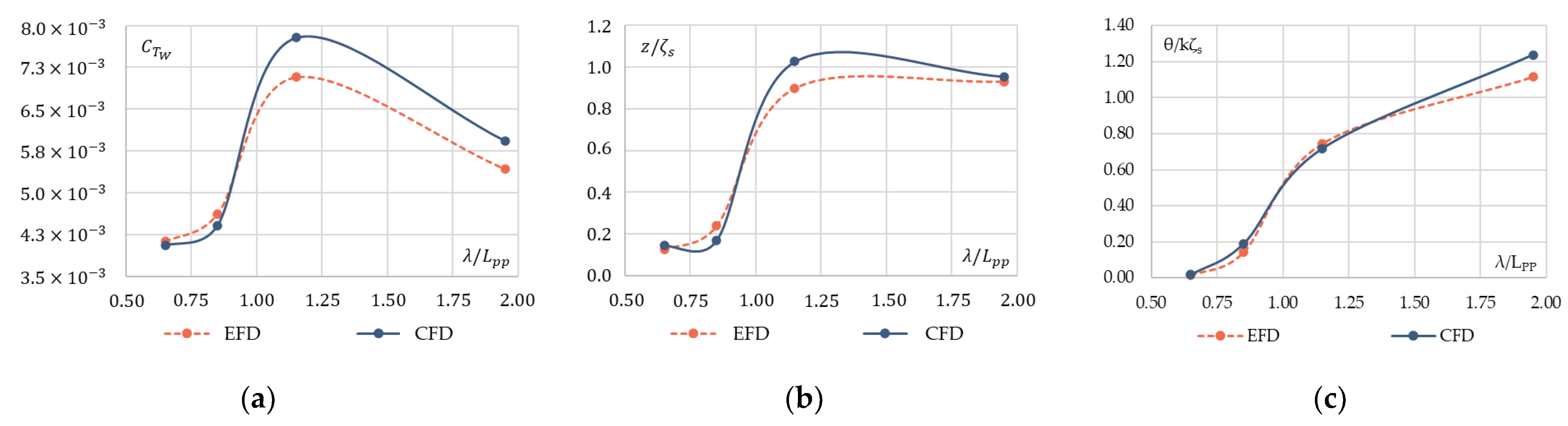
• On the validation side, the CFD results were in good agreement with EFD data, especially in terms of total resistance coefficients, with a relative difference 1.22%; however, for the vertical motions, the values were slightly significant, at 6.88% for sinkage and 3.96% for trim. This indicates that the simulation is accurate, and the result deviation is acceptable in calm water condition.
• As far as the verification study is concerned, the simulations showed a monotonic convergence for all the test cases performed in this study. The numerical errors are more affected by the grid compared to the time step. The time step convergence showed that 600 iterations per wave period is sufficient for effective prediction of the simulation parameters. Further refinement of the time step had no impact on the results. On the other hand, the grid refinement was shown to have a significant effect on the results; the finer the grid, the better the accuracy. This complies with the theory and common practice in CFD simulations.
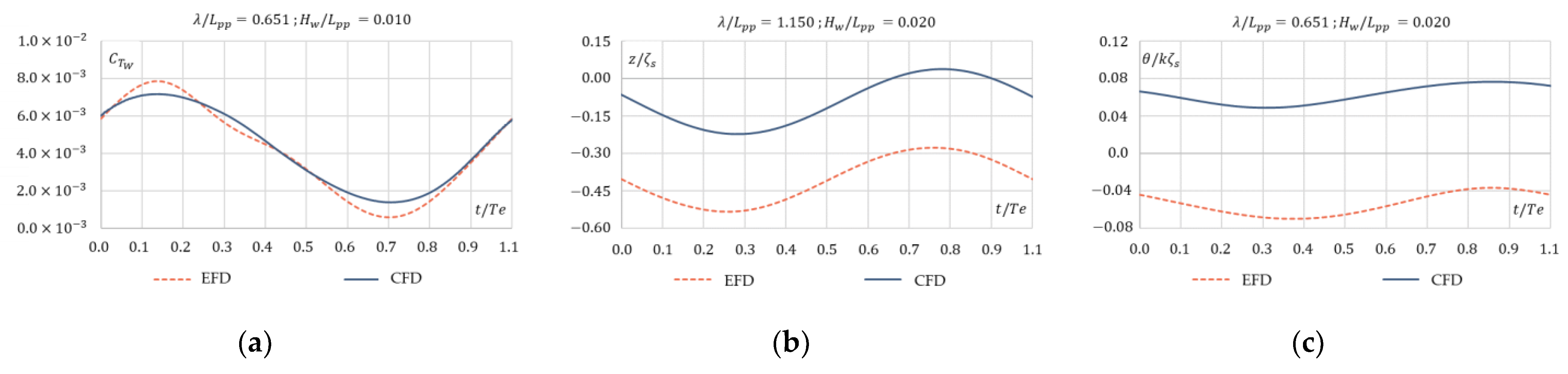
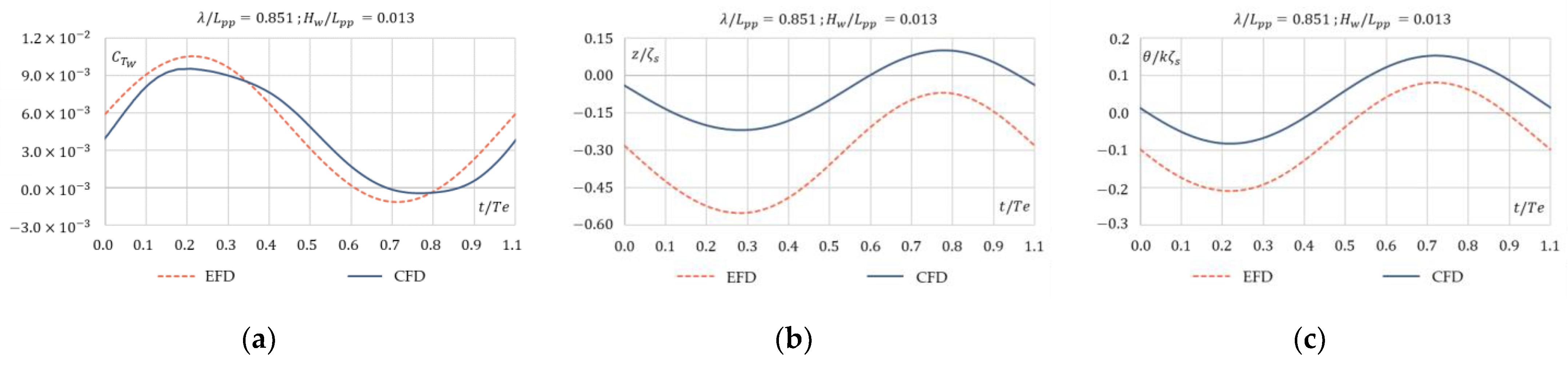
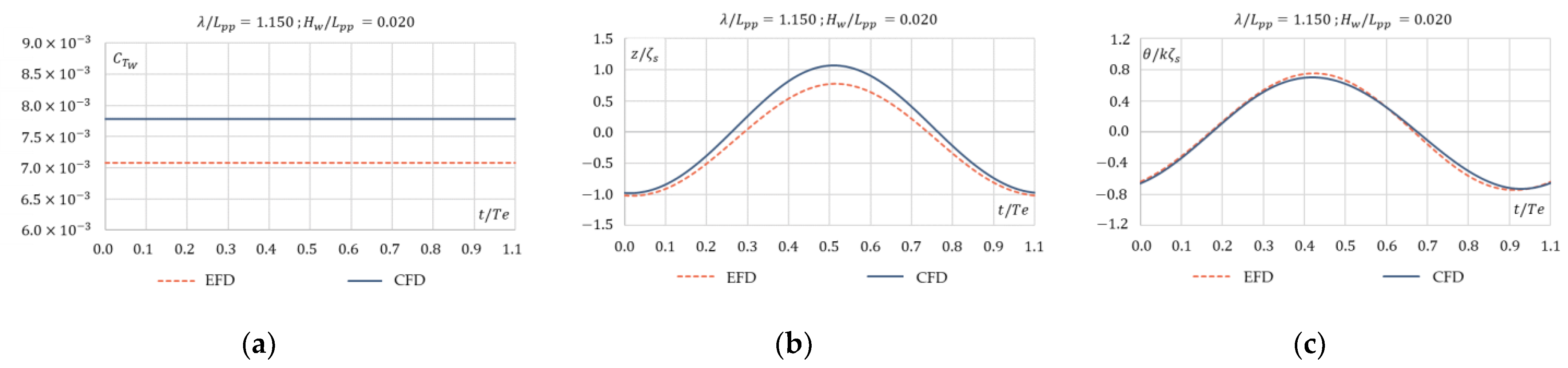
• Result validation in waves had a significant relative difference compared to that in calm water. Total resistance coefficient difference had an average value of 6.4%, while the average values for heave and pitch nondimensionalized parameters were 15.2% and 20.7%, respectively. The maximum difference for resistance was less than 10%, for heave it was within 29%, and it was within 34% for pitch motion. Though the difference between EFD and CFD was significant for ship sailing in waves, taking into consideration the fact that the study proposes a comparison between the same ship at different scales, the results were sufficient for comparative purposes, especially for the main target of the study, which is the added resistance in waves.
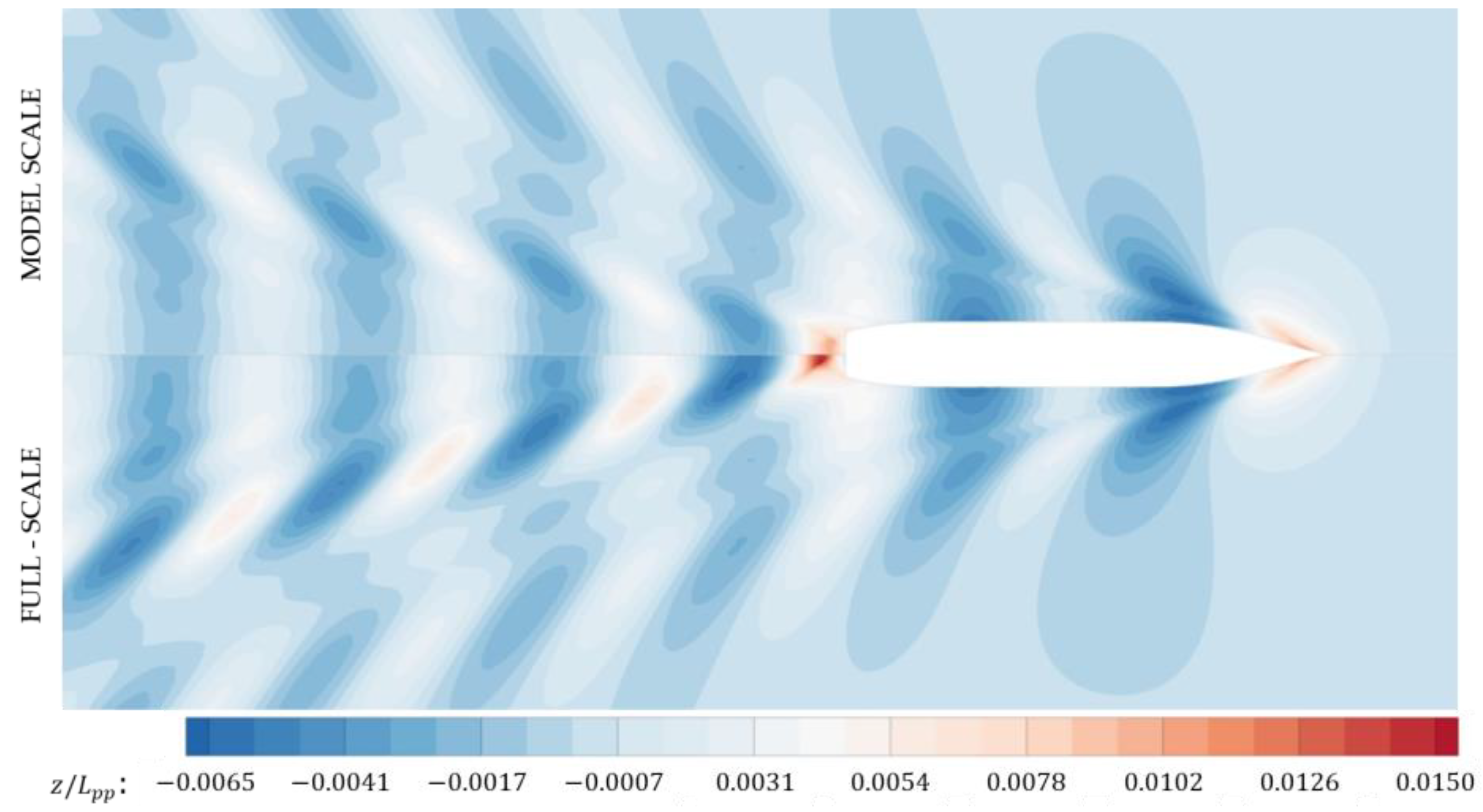
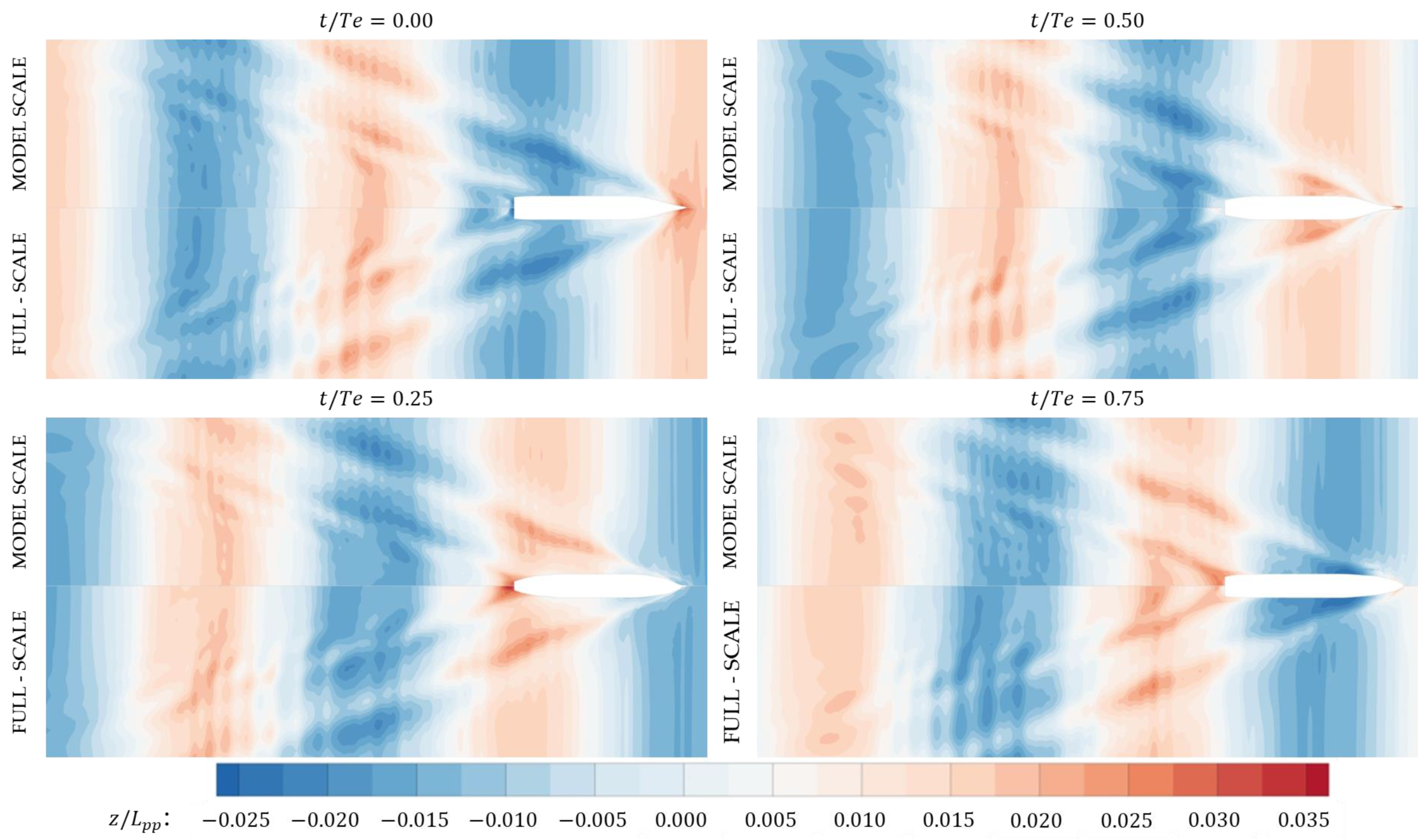
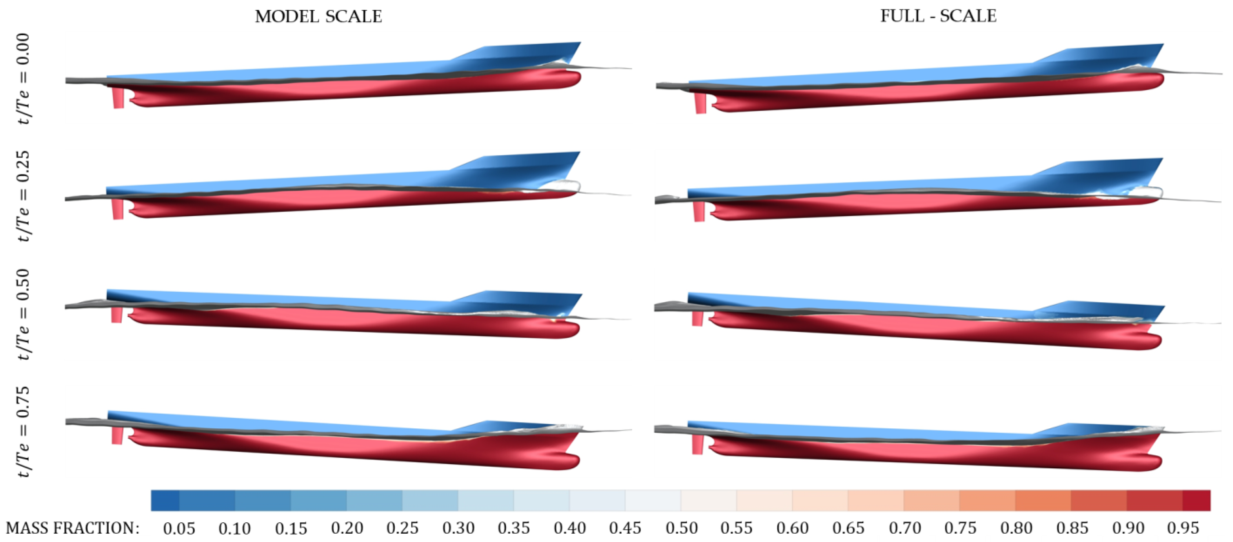
• Free-surface predictions showed that there was a slight difference observed between the model and full scale, especially at the stern zone and downstream; this was apparently related to the difference in form between model and full scale at the stern shoulders. Further investigation in that scope will be carried in separate research.
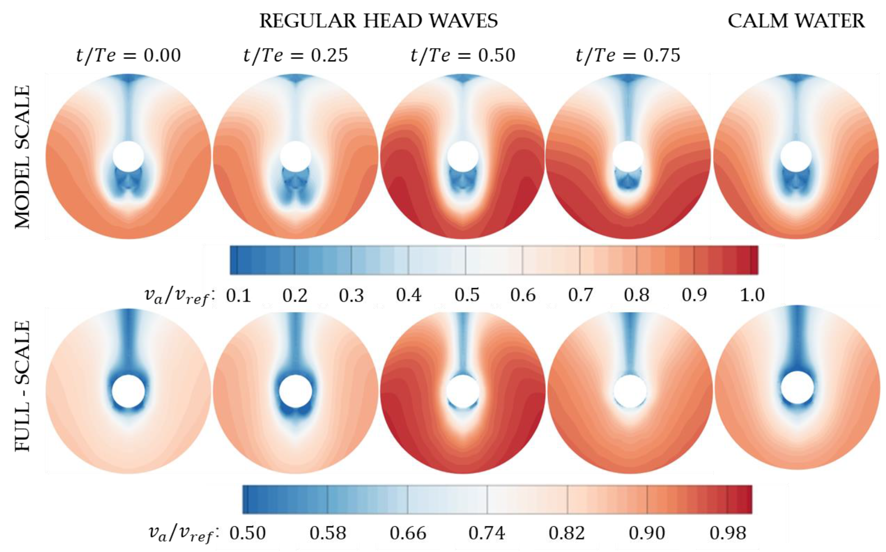
• The flow in the propeller plane was also investigated, revealing an obvious difference between model and full scale comparing the velocity contours and vortex formation in the propeller plane. The vortical formations are more significant at the model scale, while the contours are finely distributed, with fewer vortices at the full scale.
• A boundary layer fluctuation was observed as the ship sails in waves for both model and full scale. The effect was more accentuated at the model scale. Results showed that the change is significant, and may have an impact on the propulsion performance in waves. This is a subject of concern for the authors and shall be investigated in the future.

Finally, the study outcomes included promising results within the scope of the study; further investigation could be proposed to enhance the numerically obtained results, such as reducing the numerical errors by means of grid quality enhancement, improving the flow prediction using other turbulence models, and further investigation for the already encountered phenomena regarding the wake flow and free surface within the present study.

References

1. Spinelli, F.; Mancini, S.; Vitiello, L.; Bilandi, R.N.; De Carlini, M. Shipping Decarbonization: An Overview of the Different Stern Hydrodynamic Energy Saving Devices. J. Mar. Sci. Eng. 2022, 10, 574. [Google Scholar] [CrossRef]
2. Terziev, M.; Tezdogan, T.; Incecik, A. Scale effects and full-scale ship hydrodynamics: A review. Ocean Eng. 2022, 245, 110496. [Google Scholar] [CrossRef]
3. Larsson, L.; Raven, H.C. Principles of Naval Architecture: Ship Resistance and Flow; Publisher Society of Naval Architects and Marine Engineers: New Jersey, NJ, USA, 2010. [Google Scholar]
4. Raven, H.; Van der Ploeg, A.; Starke, A.R.; Eça, L. Towards a CFD-based prediction of ship performance—Progress in predicting full-scale resistance and scale effects. Int. J. Marit. Eng. 2008, 150, 31–42. [Google Scholar]
5. Terziev, M.; Tezdogan, T.; Incecik, A. A geosim analysis of ship resistance decomposition and scale effects with the aid of CFD. Appl. Ocean Res. 2019, 92, 101930. [Google Scholar] [CrossRef]
6. Pena, B.; Muk-Pavic, E.; Fitzsimmons, P. Detailed analysis of the flow within the boundary layer and wake of a full-scale ship. Ocean Eng. 2020, 218, 108022. [Google Scholar] [CrossRef]
7. Niklas, K.; Pruszko, H. Full-scale CFD simulations for the determination of ship resistance as a rational, alternative method to towing tank experiments. Ocean Eng. 2019, 190, 106435. [Google Scholar] [CrossRef]
8. Bhushan, S.; Xing, T.; Carrica, P.; Stern, F. Model and Full-Scale URANS Simulations of Athena Resistance, Powering, Seakeeping, and 5415 Maneuvering. J. Ship Res. 2009, 53, 179–198. [Google Scholar] [CrossRef]
9. Tezdogan, T.; Demirel, Y.K.; Kellett, P.; Khorasanchi, M.; Incecik, A.; Turan, O. Full-scale unsteady RANS CFD simulations of ship behaviour and performance in head seas due to slow steaming. Ocean Eng. 2015, 97, 186–206. [Google Scholar] [CrossRef]
10. Mikkelsen, H.; Shao, Y.; Walther, J.H. Numerical study of nominal wake fields of a container ship in oblique regular waves. Appl. Ocean Res. 2022, 119, 102968. [Google Scholar] [CrossRef]
11. Schuiling, B.; Lafeber, F.H.; van der Ploeg, A.; van Wijngaarden, E. The influence of the wake scale effect on the prediction of hull pressures due to cavitating propellers. In Proceedings of the Second International Symposium on Marine Propulsors, Hamburg, Germany, 15–17 June 2011. [Google Scholar]
12. Zhang, H.; Zhang, D.; Guo, C.; Wang, L.; Liu, T. Numerical analysis of the scale effect of the nominal wake field of KCS. Chin. J. Ship Res. 2017, 12, 1–7. [Google Scholar] [CrossRef]
13. Delen, C.; Bal, S. Telfer’s GEOSIM method revisited by CFD. Int. J. Marit. Eng. 2019, 161, A467–A478. [Google Scholar] [CrossRef]
14. Can, U.; Delen, C.; Bal, S. Effective wake estimation of KCS hull at full-scale by GEOSIM method based on CFD. Ocean Eng. 2020, 218, 108052. [Google Scholar] [CrossRef]
15. Guilmineau, E.; Deng, G.B.; Leroyer, A.; Queutey, P.; Visonneau, M.; Wackers, J. Influence of the turbulence closures for the wake prediction of a marine propeller. In Proceedings of the 4th International Symposium on Marine Propulsors, Austin, TX, USA, 31 May 2015. [Google Scholar]
16. Menter, F.R. Two-equation eddy-viscosity turbulence models for engineering applications. AIAA J. 1994, 32, 1598–1605. [Google Scholar] [CrossRef]
17. Rhie, C.; Chow, W.L. A numerical study of the turbulent flow past an isolated airfoil with trailing edge separation. AIAA J. 1983, 17, 1525–1532. [Google Scholar] [CrossRef]
18. Queutey, P.; Visnonneau, M. An interface capturing method for free-surface hydrodynamic flows. Comput. Fluids 2007, 36, 1481–1510. [Google Scholar] [CrossRef]
19. Queutey, P.; Visonneau, M.; Leroyer, A.; Deng, G.; Guilmineau, E. RANSE simulations of a naval combatant in head waves. In Proceedings of the 11th Numerical Towing Tank Symposium, Brest, France, 7–9 September 2008. [Google Scholar]
20. Deng, G.B.; Queutey, M.; Visonneau, M. RANS prediction of the KVLCC2 tanker in head waves. J. Hydrodyn. 2010, 22, 476–481. [Google Scholar] [CrossRef]
21. Van, S.H.; Kim, W.J.; Yim, G.T.; Kim, D.H.; Lee, C.J. Experimental Investigation of the Flow Characteristics Around Practical Hull Forms. In Proceedings of the 3rd Osaka Colloquium on Advanced CFD Applications to Ship Flow and Hull Form Design, Osaka, Japan, 25–27 May 1998. [Google Scholar]
22. Kim, W.J.; Van, S.H.; Kim, D.H. Measurement of flows around modern commercial ship models. Exp. Fluids 2001, 31, 567–578. [Google Scholar] [CrossRef]
23. Zou, L.; Larsson, L. Additional data for resistance, sinkage and trim. In Numerical Ship Hydrodynamics: An Assessment of the Gothenburg 2010 Workshop; Springer Business Media: Dordrecht, The Netherlands, 2013; pp. 255–264. [Google Scholar]
24. Simonsen, C.; Otzen, J.; Stern, F. EFD and CFD for KCS heaving and pitching in regular head waves. J. Mar. Sci. Technol. 2013, 18, 435–459. [Google Scholar] [CrossRef]
25. Hino, T.; Ster, F.; Larsson, L.; Visonneau, M.; Hirata, N.; Kim, J. (Eds.) Numerical Ship Hydrodynamics. In An Assessment of the Tokyo 2015 Workshop; Lecture Notes in Applied and Computational Mechanics; Springer Nature: Cham, Switzerland, 2021; Volume 94, pp. 61–99. [Google Scholar]
26. T2015 Workshop. Available online: http://www.t2015.nmri.go.jp (accessed on 30 December 2023).
27. ITTC. Recommended Procedures and Guidelines: Practical Guidelines for Ship CFD Applications; 7.5-03 02-03, 2011, Rev. 01; ITTC: Rio de Janeiro, Brazil, 2011; pp. 1–18.
28. Bekhit, A.; Lungu, A. URANSE simulation for the Seakeeping of the KVLCC2 Ship Model in Short and Long Regular Head Waves. In Proceedings of the IOP Conference Series: Materials Science and Engineering; IOP Publishing: Bristol, UK, 2019; Volume 591, p. 12102. [Google Scholar] [CrossRef]
29. ITTC. Recommended Procedures and Guidelines, Uncertainty Analysis in CFD Verification and Validation Methodology and Procedures; Rev. 03; ITTC: Wuxi, China, 2017; pp. 1–13.
30. Sun, W.; Hu, Q.; Hu, S.; Su, J.; Xu, J.; Wei, J.; Huang, G. Numerical Analysis of Full-Scale Ship Self-Propulsion Performance with Direct Comparison to Statistical Sea Trail Results. J. Mar. Sci. Eng. 2020, 8, 24. [Google Scholar] [CrossRef]
31. Dogrul, A.; Song, S.; Demirel, Y.K. Scale effect on ship resistance components and form factor. Ocean Eng. 2020, 209, 107428. [Google Scholar] [CrossRef]
32. Carrica, P.M.; Wilson, R.V.; Stern, F. Single-Phase Level Set Method for Unsteady Viscous Free Surface Flows. Int. J. Numer. Methods Fluids 2007, 53, 229–256. [Google Scholar] [CrossRef]
33. Nakamura, S.; Naito, S. Propulsive performance of a container ship in waves. J. Soc. Nav. Archit. Jpn. 1977, 15, 24–48. [Google Scholar]
Figure 1. Hull of the KRISO Container Ship (KCS).
Inventions 09 00022 g001
Figure 2. Computational domain and boundary conditions.
Inventions 09 00022 g002
Figure 3. Computational grid. (a) Coarse grid; (b) medium grid; (c) fine grid.
Inventions 09 00022 g003
Figure 4. Comparison between CFD and EFD curves for (a) total resistance coefficient in waves, (b) heave amplitude, and (c) pitch amplitude.
Inventions 09 00022 g004
Figure 5. Comparison between CFD and EFD curves for (a) total resistance coefficient in wave amplitude, (b) heave amplitude, and (c) pitch amplitude for λ / L p p = 0.651 and H w / L p p = 0.010 .
Inventions 09 00022 g005
Figure 6. Comparison between CFD and EFD curves for (a) total resistance coefficient in wave amplitude, (b) heave amplitude, and (c) pitch amplitude for λ / L p p = 0.851 and H w / L p p = 0.013 .
Inventions 09 00022 g006
Figure 7. Comparison between CFD and EFD curves for (a) average total resistance coefficient in waves, (b) heave amplitude, and (c) pitch amplitude for λ / L p p = 1.150 and H w / L p p = 0.020 .
Inventions 09 00022 g007
Figure 8. Comparison between CFD and EFD curves for (a) total resistance coefficient in wave amplitude, (b) heave amplitude, and (c) pitch amplitude for λ / L p p = 1.951 and H w / L p p = 0.032 .
Inventions 09 00022 g008
Figure 9. Comparison between model-scale and full-scale curves for wave added resistance coefficient in the case of (a) H w / L p p = 0.010 , (b) H w / L p p = 0.020 , and (c) H w / L p p = 0.032 .
Inventions 09 00022 g009
Figure 10. Comparison between model-scale and full-scale curves for heave amplitude in the case of (a) H w / L p p = 0.010 , (b) H w / L p p = 0.020 , and (c) H w / L p p = 0.032 .
Inventions 09 00022 g010
Figure 11. Comparison between model-scale and full-scale curves for pitch amplitude in the case of (a) H w / L p p = 0.010 , (b) H w / L p p = 0.020 , and (c) H w / L p p = 0.032 .
Inventions 09 00022 g011
Figure 12. Comparison between model scale and full scale for wave elevation in calm water.
Inventions 09 00022 g012
Figure 13. Comparison between model scale and full scale for wave elevation in regular head waves for λ / L p p = 1.951 and H w / L p p = 0.032 .
Inventions 09 00022 g013
Figure 14. Comparison between model scale and full scale for mass fraction distribution in regular head waves for λ / L p p = 1.951 and H w / L p p = 0.032 .
Inventions 09 00022 g014
Figure 15. Comparison between model scale and full scale for axial velocity in the propeller in regular head waves for λ / L p p = 1.951 and H w / L p p = 0.032 . Section at propeller plane.
Inventions 09 00022 g015