


Modeling and Simulation of a 2SPU-RU Parallel Mechanism for a Prosthetic Ankle with Three Degrees of Freedom


Abstract
1. Introduction
- The model uniquely simulates essential ankle movements, tailored specifically for ankle prostheses.
- The integration of parallel mechanisms to enhance prosthetic stability and adaptability using the innovative 2SPU-RU parallel mechanism.
- The design is rigorously validated against theoretical and simulation results to ensure its effectiveness and accuracy.
2. Biomechanical Principles
2.1. Planes, Axes, and Types of Movement
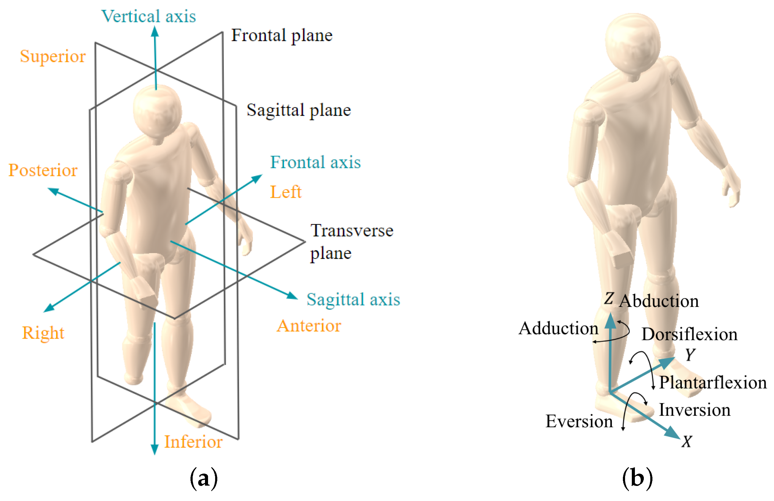
- Anatomical plane: The sagittal plane is a vertical division of the body into right and left sections, with movement occurring around a horizontal axis. The frontal plane, called the coronal plane, splits the body into anterior (front) and posterior (back) parts. Meanwhile, the horizontal transverse plane divides the body into superior (upper) and inferior (lower) sections, as shown in Figure 1a.
- Anatomical axes: The vertical axis runs from top to bottom and serves as the axis of rotation for movements occurring in the transverse plane. The sagittal axis, which extends from front to back, is linked with movements in the frontal plane, such as lateral bending to the side. Meanwhile, the frontal axis runs from side to side through the body and facilitates movements in the sagittal plane, as shown in Figure 1a.
- Anatomical motions: Plantarflexion involves moving the foot away from the body by pointing the toes downward, while dorsiflexion is the opposite movement, flexing the foot upward toward the shin. Eversion occurs when the sole is turned outward, away from the body’s median plane, and inversion is when the sole turns inward toward the median plane. Abduction refers to moving the foot away from the body’s midline in the transverse plane, and adduction is the foot’s movement toward the body’s midline in the same plane, as shown in Figure 1b.
2.2. The Gait Cycle
3. Design of a Parallel 2SPU-RU Mechanism
4. Inverse Kinematic Analysis
4.1. Global and Local Reference Frame
- The origin is located at the geometric center of the fixed platform.
- The axis in the anteroposterior direction (from the heel to the tip of the foot). It is the main direction of advance when walking.
- The axis in the mediolateral direction; that is, perpendicular to the sagittal plane of the body and horizontal to the ground, pointing toward the foot’s outer side.
- The axis in the vertical direction, upward. This axis will mainly align with the body weight and the reactive force of the ground.
4.2. Geometric Parameters
- (a)
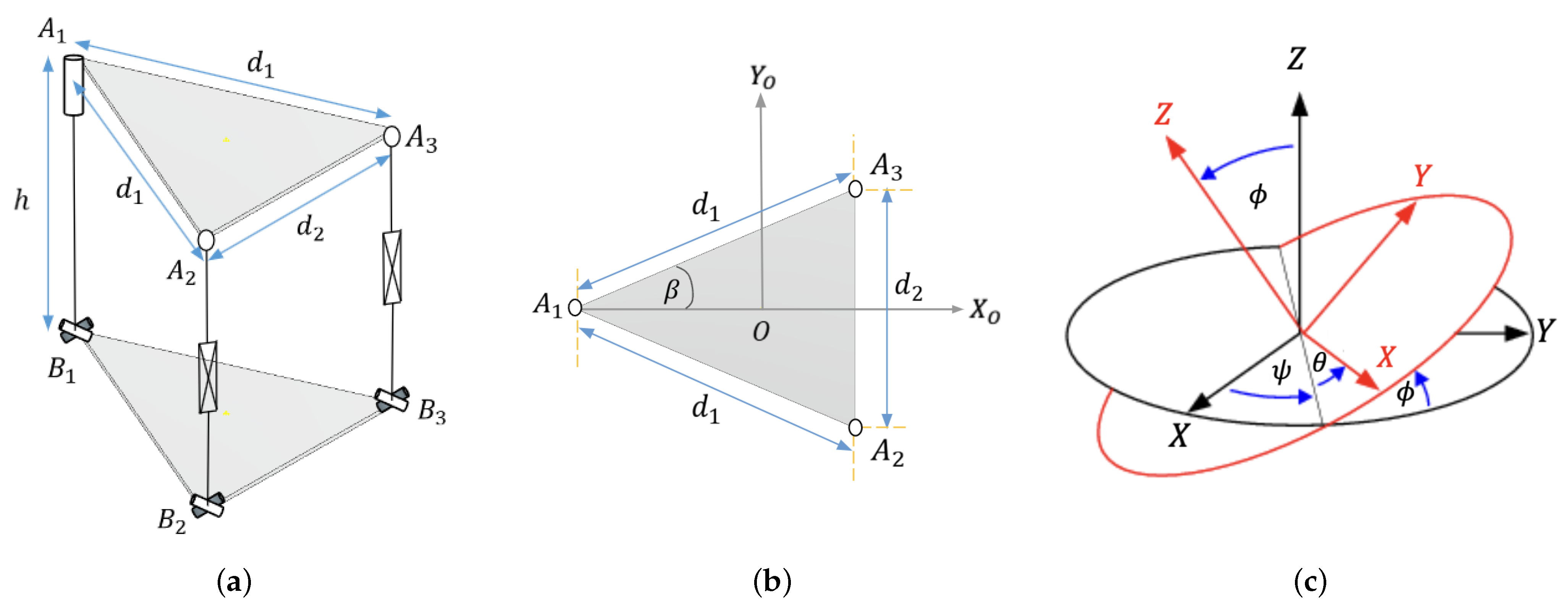
- Distances Between JointsThe distances between the joints, as shown in Figure 8a, are linear measurements that indicate the separation between various connecting joints of the parallel mechanism. These distances define the geometric configuration of the mechanism and influence its range of movement. The platforms and are rigid elements shaped into an isosceles triangle. The triangles and are identical. The side lengths , and , are equal, respectively.
- (b)
- Joint CoordinatesThe coordinates of the joints in the parallel mechanism represent the spatial positions of the fixed and moving platforms’ kinematic pairs. These coordinates are defined within a global reference frame and are used to describe each joint’s position and relative orientation in space. Figure 8b details the coordinates of the points O, , , , which make up the 2SPU-RU parallel mechanism.
- (c)
- Angular Parameters of the Moving PlatformIn the parallel mechanism, the orientation of the moving platform is defined using the Bryant–Cardan ZXY angle sequence, as shown in Figure 8c. This method starts with a rotation around the Z axis by an angle , followed by a rotation around the X axis by an angle , and culminates with a rotation around the Y axis by an angle , as detailed in Equation (1). The choice of the ZXY sequence is supported by recommendations from the International Society of Biomechanics, which proposes this specific ZXY sequence to calculate ankle rotations. In anatomical terms, this sequence corresponds to the movements of adduction–abduction, inversion–eversion, and plantarflexion–dorsiflexion:
- (d)
- Angular Velocity of the Moving PlatformThe angular velocity vector depends on the time variation of the rotation matrix composed of the angles , , . In this case, the angular velocity is obtained through Equation (2):
- (e)
- Angular Acceleration of the Moving PlatformThe angular acceleration of the moving platform is obtained by differentiating the angular velocity for time, as shown in Equation (3):
4.3. First Kinematic Chain
- (a)
- Position AnalysisThe position vectors of the RU kinematic chain are defined to the global reference frame O(), as shown in Figure 9a. The position vectors define the vector Equation (4).Where the vectors , , and remain constant, which implies that their components do not change concerning time or any other variable, and is the ankle’s rotation angle in the rotation axis of the moving platform:where is the vector representing the position of the spherical joint to the origin O, is the vector representing the position of the rotary actuator to , and is the vector representing the position of P located at the universal joint U concerning the origin O.
- (b)
- Linear and Angular Velocity AnalysisThe linear and angular velocity of the kinematic chain RU is analyzed. It is important to note that all the bodies of each kinematic chain i (with ) move with the same angular velocity. The rotary actuator belongs to the kinematic chain RU and is at point . This implies that the vector connecting with maintains a constant magnitude and direction. Therefore, it is established that the derivative of the position vector = is equal to zero .Furthermore, due to the connection with the universal joint (U) of two degrees of freedom located at , it is established that the rotation on the axis of the rotary actuator coincides with the rotation of the moving platform concerning the axis. It corresponds to the first rotation of the three successive intrinsic rotations that define the rotation matrix of the moving platform through Equation (1). Thus, the angular velocity of the actuator is equal to the derivative of the rotation angle with respect to the axis (), as shown in Figure 9b.
- (c)
- Angular Acceleration AnalysisBy differentiating the equation that relates the angular velocity of the kinematic chain RU with the velocity of the moving platform projected onto the axis , it is obtained that . That is to say, the angular acceleration of the kinematic chain RU is equal to the angular acceleration of the second derivative of the rotation angle concerning the axis.
4.4. Second and Third SPU Kinematic Chains
- (a)
- Position Analysis of the ith SPU Kinematic ChainThe position vectors of the SPU kinematic chain are established to the global reference frame O(), as depicted in Figure 10a. This results in Equation (5), which equals the sum of the vectors , , and the vectors and :where is the vector representing the position of the spherical joint to the origin O, is the vector representing the position of the rotary actuator to , and is the vector representing the position of the universal joint with respect to .From Equation (5), the vector has a magnitude presented in Equation (6) and a direction presented in Equation (7):In Figure 10b, a linear actuator composed of a cylinder and a piston is illustrated, where the latter moves along the axis, defined along the unit vector . The axis is defined along the second axis of rotation of the universal joint, which allows for relative rotation between the second kinematic chain and the universal joint.From the global reference frame O(, , ) of the fixed platform, the position vectors of the center of mass of the cylinder and the piston are defined, which are denominated and and are defined by Equation (8) and Equation (9), respectively. The distance between and the center of mass of the cylinder is represented by e, while the distance between and the center of mass of the piston is designated as f:
- (b)
- Linear Velocity Analysis of the ith Kinematic Chain SPUThe velocity analysis aims to determine a mechanical element’s linear and angular velocities. Starting from Equation (5), the terms on the left side of the equality are derived, resulting in Equation (10).Where is the velocity vector of the universal joint , is the velocity of the universal joint (which is always zero), and the term represents the cross product between the angular velocity of the mobile platform and the vector :The velocity is transformed to the local reference frame of the ith kinematic chain , which is expressed with a left superscript, resulting in Equation (11).Where is the rotation matrix from the global reference frame O(,, ) to the local reference frame of the ith kinematic chain:Equation (12) is used to calculate :where is the rotation matrix from the local reference frame of the kinematic chain to the local reference frame of the moving platform . The rotation matrix is determined by two rotations: is the rotation around the axis, followed by the rotation around the axis, and it is calculated in Equation (13):It is noted that the third column of the matrix equals the negative of the vector expressed in the reference frame of the moving base . Therefore, to resolve Equation (13), the angles were calculated according to Equation (14):where is the negative vector of the vector , expressed in the reference frame of the moving platform .The terms found on the left side of Equation (5) are derived and equal to the velocity . This equality relates the speed of the universal joint with the angular velocity and the linear speed of the kinematic chain .The new equation expressed in the local reference frame allows us to obtain a direct expression of the angular velocity of the second kinematic chain according to Equation (17):
- (c)
- Angular Velocity Analysis of the ith Kinematic Chain SPUThe angular velocity of the ith kinematic chain with respect to the local reference frame is calculated by multiplying by the cross product of in both terms of Equation (17):The last term of Equation (19) is eliminated because the unit vectors are parallel, resulting in a cross product equal to zero. Similarly, in the Equation, the property of the vector cross product is applied, resulting in Equation (20):In Equation (20), the term is equal to one by the dot product between the unit vectors.
- (d)
- Linear Velocity Analysis of the Cylinder and Piston in the Linear ActuatorOnce the linear velocity of the universal joint and the angular velocity of the ith kinematic chain relative to the local reference frame (, , ) are known, it is possible to calculate the velocity of each component within the ith kinematic chain to the local reference frame (, , ). The cylinder’s velocity is denoted by and the piston’s velocity by .The terms and are replaced in Equation (26):The term is factored out in Equation (27):
- (e)
- Linear Acceleration Analysis of the ith Kinematic Chain SPUDifferentiating Equation (10) concerning time yields the acceleration of point as defined by Equation (28):The velocity is expressed in the reference frame of the kinematic chain (, , ), resulting in Equation (29):The acceleration of point in Equation (30) is expressed in terms of the kinematic chain acceleration using the derivative of Equation (17):The terms and from Equation (31) are zero because the dot product of two perpendicular vectors is zero.Likewise, for the term , the property is applied, and Equation (32) is obtained:
- (f)
- Angular Acceleration Analysis of the ith Kinematic Chain SPUThe term of Equation (35) is zero due to the cross product of two parallel vectors.In the terms , , and the property of the cross product , Equation (21), and deriving Equation (21) are applied, reducing to
- (g)
- Linear Acceleration Analysis of the Cylinder and Piston of the Linear Actuator
5. Jacobian Matrices
5.1. Jacobian Matrix of Kinematic Chain RU
5.2. The Moving Platform
5.3. Second and Third Kinematic Chain SPU
6. Inverse Dynamics Analysis
6.1. External Forces and Moments on the Moving Platform
- (a)
- Forces and Inertia on the Kinematic Chain RUAssuming that gravitational force is the only external force, the resultant applied forces and inertia exerted at the center of mass of the link in the kinematic chain RU can be expressed in the local frame with Equation (58):where is the vector of resultant forces and moments on the link of the first kinematic chain, expressed from the local reference frame ; is the mass of the link of the kinematic chain RU in [kg]; and is the moment of inertia of the link of the kinematic chain RU [kg·m2].
- (b)
- Forces and Inertia on the Second Kinematic Chain (SPU)Similarly, assuming that gravitational force is the only external force, the resultant applied forces and inertia exerted on the centers of mass of the cylinder and piston can be expressed in the local frame of the second kinematic chain with Equations (59) and (60):where is the vector of resultant forces and moments on the cylinder of the second kinematic chain (SPU), expressed from the local reference frame ; is the mass of the cylinder of the second kinematic chain (SPU) in [kg]; and is the moment of inertia of the cylinder of the second kinematic chain (SPU) concerning the local reference frame , [kg·m2]:where is the vector of resultant forces and moments on the piston of the second kinematic chain (SPU), expressed from the local reference frame . is the mass of the piston of the second kinematic chain (SPU), [kg]. is the moment of inertia of the piston of the second kinematic chain (SPU) concerning the local reference frame , [kg·m2].
6.2. Motion Equations
7. Results
7.1. Simulation Parameters
- (a)
- Joint coordinates: The coordinates of the fixed platform in millimeters were obtained from the global reference frame O(, , ):The moving platform’s coordinates were obtained from its reference frame (, , ).
- (b)
- Mass properties: The moving platform mass is 0.22 kg. The mass of the cylinder in the second kinematic chain is 0.085 kg, and the piston in the same chain has a mass of 0.010 kg. Similarly, the cylinder mass is 0.085 kg for the third kinematic chain, and the piston is 0.010 kg. Lastly, the mass of the link in the kinematic chain RU is 0.21 kg.
- (c)
- Center of mass of cylinder and piston: The distance between and the center of mass of cylinder 2 is e = 55 mm. The distance between and the center of mass of piston 2 is f = 27 mm. The distance between and the center of mass of cylinder 3 is e = 55 mm. The distance between and the center of mass of piston 3 is f = 27 mm.
- (d)
- Inertial properties in kg.mm2:
- (e)
- Gravity vector: .
- (f)
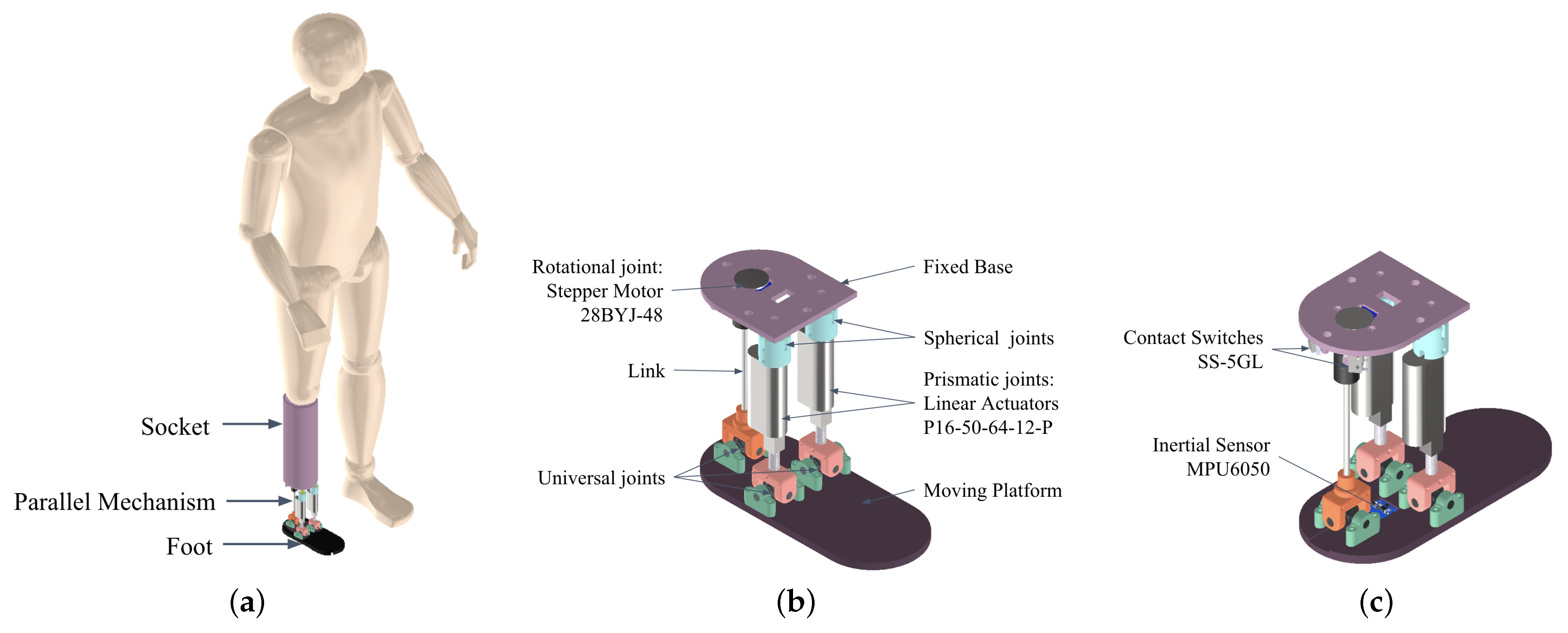
- External force: The reaction forces on the ground during a gait are forces external and . Here, force is the vertical force on the Z axis and force is the horizontal reaction force from the ground on the X axis. Additionally, the external moment = exists, as shown in Figure 3.
7.2. Inverse Kinematics Results in MATLAB R2022b
7.3. Inverse Kinematics Simulating in Simscape
7.4. Inverse Dynamics Results in MATLAB and Simscape
8. Discussion
- Rotation angle of the rotary actuator: Figure 11a shows the rotation angle of the rotary actuator in MATLAB. During initial contact (IC) and load response (LR), the angle decreases to approximately −5.5°, followed by a significant increase to around 8.6° during the initial swing (ISw) phase. This behavior is crucial for replicating the natural ankle movement, where the combined ankle movement (plantarflexion–dorsiflexion, inversion–eversion, and abduction–adduction) is essential for efficient gait.
- Length of the linear actuators: Figure 11b shows the variation in the length of linear actuators 2 and 3 in MATLAB. The most notable differences are seen during the initial swing (ISw), where actuator 2 increases in length up to 48 mm, while actuator 3 reaches only 42 mm. This variation can be attributed to rotation angles of the biomechanical data from the gait cycle, which reflect differences in each actuator. These differences highlight how various parameters can influence ankle movement.
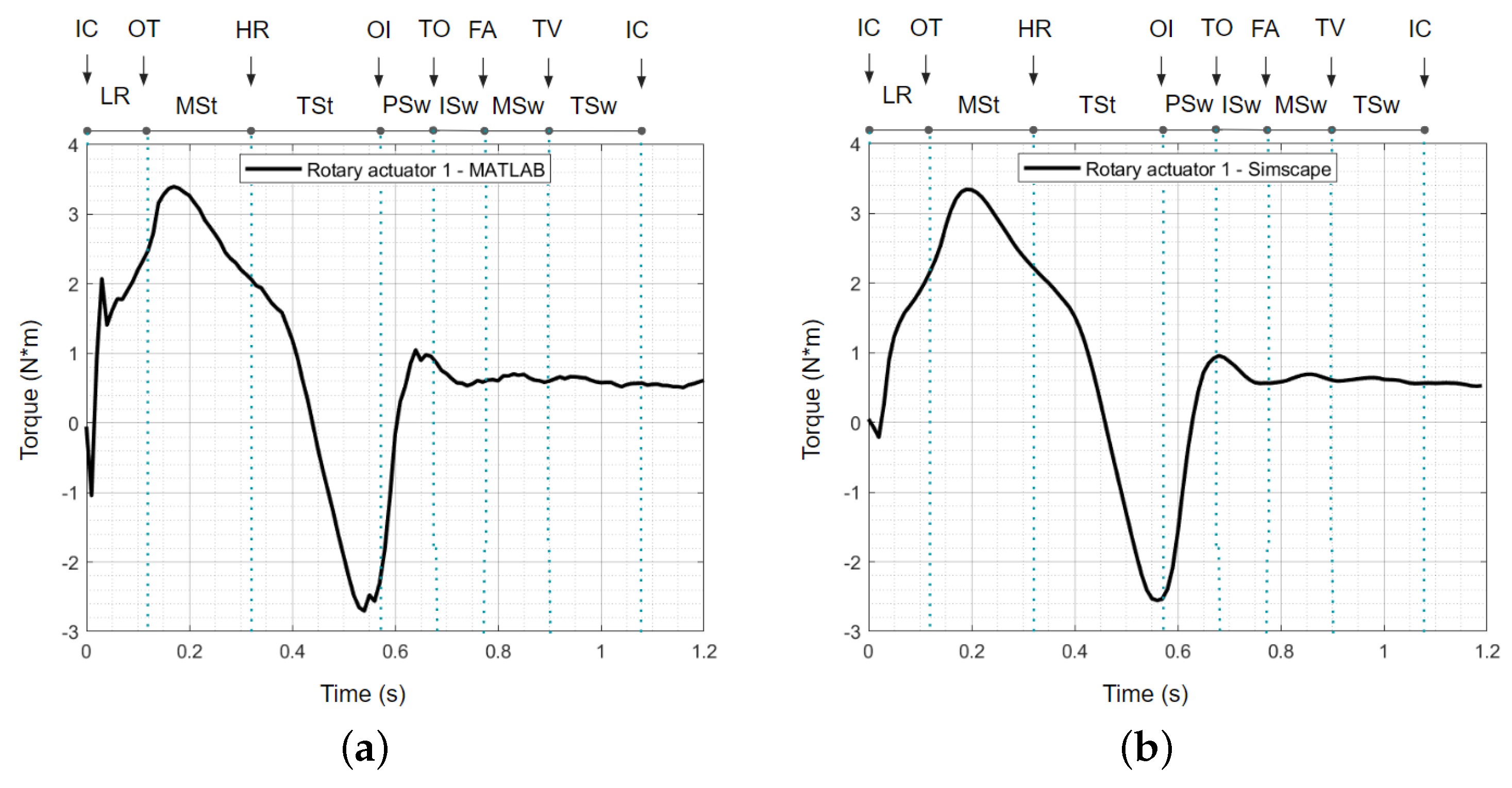
- Torque of the rotary actuator: Figure 13 compares torque from the rotary actuator obtained from MATLAB and Simscape. The observed torque patterns are remarkably similar between both simulations. During the initial contact (IC) and load response (LR) phases, a rapid increase in torque is observed, peaking around 3.5 Nm, followed by a drop to negative values during terminal stance (TSt) and pre-swing (PSw). This consistency suggests that both simulation environments can accurately model the torque dynamics in the rotary actuator.
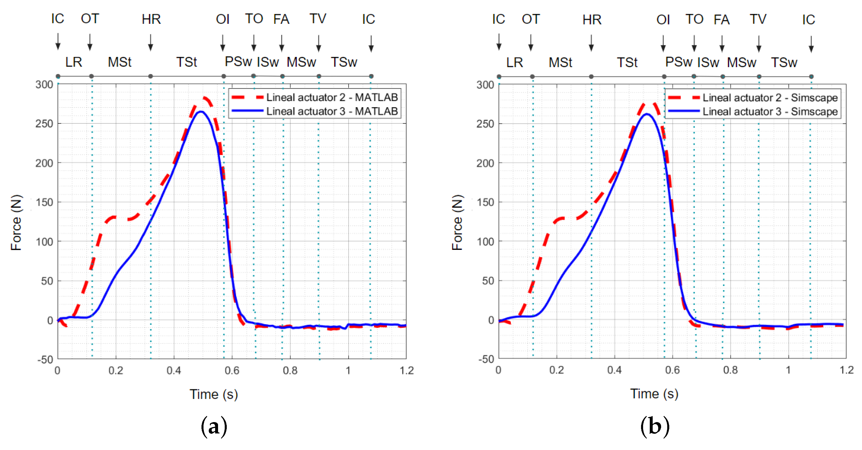
- Force of the linear actuators: Figure 14 presents the forces generated by linear actuators 2 and 3 in MATLAB and Simscape. Similar to the torque analysis, the recorded forces show similar patterns in both simulations. During the load response (LR) phase, the force peaks around 280 N for actuator 2 and 260 N for actuator 3, consistent across both platforms. This behavior indicates that both MATLAB and Simscape can adequately replicate the forces involved in the gait cycle using linear actuators.
- Implications and limitations: The similarities observed between MATLAB and Simscape in modeling torque and force suggest that both environments can be reliably used for biomechanical studies of the gait cycle. However, the differences in the lengths of the linear actuators during the initial swing (ISw) phase indicate that fine-tuning parameters and configurations are needed to achieve precise replication of ankle movement. A limitation of the study is the reliance on simulation models, which may only capture some of the complexities of human movement. Future research could integrate experimental data to validate and adjust simulation models, ensuring greater accuracy in representing biomechanical behavior.
- Uncertainty: The 2SPU-RU parallel mechanism, used in three-degree-of-freedom ankle prostheses, can present significant challenges during its manufacturing process. These uncertainties may arise from various sources, such as errors in the manufacturing parameters of the mechanism’s components and unexpected flexibility of the elements within the kinematic chain that may deviate from the theoretical design. Such variations can affect the precision and dynamic behavior of the mechanism, complicating the prosthesis’s functionality. To mitigate these potential issues, it is crucial to adopt strategies such as rigorous calibration and integrating sensors for real-time feedback, enabling dynamic adjustments to control the parameters. A sensitivity analysis will also help understand how different uncertainties impact the mechanism’s performance.
- Specific application in ankle prostheses: Unlike general existing approaches applicable across a broad range of nonlinear systems, our model is designed and optimized for the biomechanics and needs of the human ankle. This includes the precise simulation of plantarflexion–dorsiflexion, eversion–inversion, and abduction–adduction movements, crucial for mimicking the natural ankle’s functionality.
- Integration of parallel mechanisms in ankle prostheses: Our study addresses a significant gap in the current literature by integrating parallel mechanisms into the design of ankle prostheses, which not only enhances stability and precision but also facilitates dynamic adaptation to different terrains and movements. This adaptability is achieved through the unique configuration of the 2SPU-RU mechanism, providing superior balance and control compared to traditional designs.
- Validation through dynamic modeling and simulation: We extensively validated our model, comparing theoretical and simulated results to ensure accuracy and applicability. This rigorous validation demonstrates the effectiveness of our design under realistic operating conditions, which is often a challenge with more abstract theoretical approaches.
9. Conclusions
Author Contributions
Funding
Data Availability Statement
Conflicts of Interest
Abbreviations
| a1 | the vector representing the position of the spherical joint to the origin O. |
| s1 | the vector representing the position of the rotary actuator to . |
| p | the vector representing the position of P located at the universal joint U with respect to the origin O |
| the rotation angle of the link of the kinematic chain RU. | |
| ai | the vector representing the position of the spherical joint to the origin O. |
| si | the vector representing the position of the rotary actuator to . |
| bi | the vector representing the position of the universal joint with respect to . |
| the velocity vector of the universal joint . | |
| the velocity of the universal joint (which is always zero). | |
| the angular velocity of the moving platform. | |
| the rotation matrix from the global reference frame O(,, ) to the local reference frame of the kinematic chain i. | |
| the six-row vector that represents the linear and angular velocities of the moving platform expressed in the global reference frame . | |
| the six-row vector that represents the linear and angular velocities of the link of the kinematic chain RU expressed in the local reference frame . | |
| the Jacobian matrix of the link of the kinematic chain RU. | |
| the Jacobian matrix such that . | |
| the Jacobian matrix such that . | |
| the third row of the Jacobian matrix . | |
| the Jacobian matrix of the ith kinematic chain. | |
| the Jacobian matrix of the ith kinematic chain expressed in its local reference frame (, , ). | |
| the Jacobian matrix of actuator i. | |
| the Jacobian matrices of the cylinder of the ith kinematic chain. | |
| the Jacobian matrices of the piston of the ith kinematic chain. | |
| the vector of forces and resulting moments on the moving platform. | |
| the external force exerted at the center of mass of the moving platform, [N]. | |
| the external moment exerted at the articulation between the moving platform and kinematic chain 1, . | |
| the mass of the moving platform, [kg]. | |
| the gravity vector . | |
| the inertia matrix of the moving platform taken about the center of mass and expressed in the fixed frame O , [kg·m2]. | |
| the linear acceleration of the center of gravity of the moving platform, . | |
| the vector of resultant forces and moments on the link of the first kinematic chain, expressed from the local reference frame . | |
| the mass of the link of the kinematic chain RU, [kg]. | |
| the moment of inertia of the link of the kinematic chain RU, [kg·m2]. | |
| the vector of resultant forces and moments on the cylinder of the second kinematic chain (SPU), expressed from the local reference frame . | |
| the vector of resultant forces and moments on the piston of the second kinematic chain (SPU), expressed from the local reference frame . | |
| the mass of the cylinder of the second kinematic chain (SPU), [kg]. | |
| the mass of the piston of the second kinematic chain (SPU), [kg]. | |
| the moment of inertia of the cylinder of the second kinematic chain (SPU) with respect to the local reference frame , [kg·m2]. | |
| the moment of inertia of the piston of the second kinematic chain (SPU) with respect to the local reference frame , [kg·m2]. | |
| the vector of the rotation angle of the link of the kinematic chain RU and the lengths of the second and third kinematic chains , respectively. | |
| the vector of the torques applied to the revolute joints and two prismatic joints. | |
| the position vector of the moving platform. | |
| the position vector of the link of the kinematic chain RU. | |
| the position vector of the cylinder of the kinematic chain i (2 or 3). | |
| the position vector of the piston of the kinematic chain i (2 or 3). |
References
- Sathsara, A.K.P.; Widanage, K.N.D.; Sooriyaperakasam, N.; Ranaweera, R.K.P.S.; Gopura, R.A.R.C. A Hybrid Powering Mechanism for a Transtibial Robotic Prosthesis. In Proceedings of the 2019 Moratuwa Engineering Research Conference (MERCon), Moratuwa, Sri Lanka, 3–5 July 2019; pp. 447–453. [Google Scholar] [CrossRef]
- World Health Organization. WHO Standards for Prosthetics and Orthotics; World Health Organization: Geneva, Switzerland, 2017; ISBN 978-92-4-151248-0. License: CC BY-NC-SA 3.0 IGO; Available online: https://www.who.int/publications/i/item/9789241512480 (accessed on 24 June 2024).
- Ying, A.F.; Tang, T.Y.; Jin, A.; Chong, T.T.; Hausenloy, D.J.; Koh, W.P. Diabetes and other vascular risk factors in association with the risk of lower extremity amputation in chronic limb-threatening ischemia: A prospective cohort study. Cardiovasc. Diabetol. 2022, 21, 7. [Google Scholar] [CrossRef] [PubMed]
- Abarca, V.E.; Gallardo, N.J.; Elías, D.A. Mecanismo paralelo UPS-1S para la articulación de un tobillo protésico para personas con amputación transtibial. Col. Investig. Multidisc. 2019, 7, 1. [Google Scholar]
- Salazar, C.A.; Abarca, V.E. Design of a Mechanism for a Robotic Transtibial Prosthesis. Int. J. Sci. Technol. Res. 2019, 8, 1416–1422. [Google Scholar]
- Barnes, J.A.; Eid, M.A.; Creager, M.A.; Goodney, P.P. Epidemiology and Risk of Amputation in Patients with Diabetes Mellitus and Peripheral Artery Disease. Arterioscler. Thromb. Vasc. Biol. 2020, 40, 1808–1817. [Google Scholar] [CrossRef] [PubMed]
- Boyko, E.J.; Monteiro-Soares, M.; Wheeler, S.G.B. Peripheral Arterial Disease, Foot Ulcers, Lower Extremity Amputations, and Diabetes. In Diabetes in America; Cowie, C.C., Casagrande, S.S., Menke, A., Eds.; National Institute of Diabetes and Digestive and Kidney Diseases (US): Bethesda, MD, USA, 2018; Chapter 20. Available online: https://www.ncbi.nlm.nih.gov/books/NBK567977/ (accessed on 3 January 2024).
- Chihuri, S.; Wong, C.K. Factors Associated with the Likelihood of Fall-Related Injury among People with Lower Limb Loss. Inj. Epidemiol. 2018, 5, 42. [Google Scholar] [CrossRef] [PubMed]
- Itsiopoulos, I.; Vasiliadis, A.V.; Tsitouras, D.; Goulas, P.; Malliou, P.; Ktenidis, K. Amputation in Necrotizing Fasciitis - Dilemma or Reality: A Case Report and Literature Review. J. Orthop. Case Rep. 2020, 10, 54–58. [Google Scholar] [PubMed]
- Parsons, C.M.; Pimiento, J.M.; Cheong, D.; Marzban, S.S.; Gonzalez, R.J.; Johnson, D.; Letson, G.D.; Zager, J.S. The Role of Radical Amputations for Extremity Tumors: A Single Institution Experience and Review of the Literature. J. Surg. Oncol. 2012, 105, 149–155. [Google Scholar] [CrossRef]
- Alessa, M.; Alkhalaf, H.A.; Alwabari, S.S.; Alwabari, N.J.; Alkhalaf, H.; Alwayel, Z.; Almoaibed, F. The Psychosocial Impact of Lower Limb Amputation on Patients and Caregivers. Cureus 2022, 14, e31248. [Google Scholar] [CrossRef]
- Gonzales-Huisa, O.A.; Oshiro, G.; Abarca, V.E.; Chavez-Echajaya, J.G.; Elias, D.A. EMG and IMU Data Fusion for Locomotion Mode Classification in Transtibial Amputees. Prosthesis 2023, 5, 1232–1256. [Google Scholar] [CrossRef]
- Roșca, A.C.; Baciu, C.C.; Burtăverde, V.; Mateizer, A. Psychological Consequences in Patients with Amputation of a Limb. An Interpretative-Phenomenological Analysis. Front. Psychol. 2021, 12, 537493. [Google Scholar] [CrossRef]
- Gavette, H.; McDonald, C.L.; Kostick-Quenet, K.; Mullen, A.; Najafi, B.; Finco, M.G. Advances in Prosthetic Technology: A Perspective on Ethical Considerations for Development and Clinical Translation. Front. Rehabil. Sci. 2024, 4, 1335966. [Google Scholar] [CrossRef] [PubMed]
- Manz, S.; Valette, R.; Damonte, F.; Gaudio, L.A.; Gonzalez-Vargas, J.; Sartori, M.; Dosen, S.; Rietman, J. A Review of User Needs to Drive the Development of Lower Limb Prostheses. J. NeuroEng. Rehabil. 2022, 19, 119. [Google Scholar] [CrossRef] [PubMed]
- van Schaik, L.; Hoeksema, S.; Huvers, L.F.; Geertzen, J.H.B.; Dijkstra, P.U.; Dekker, R. The most important activities of daily functioning: The opinion of persons with lower limb amputation and healthcare professionals differ considerably. Int. J. Rehabil. Res. 2022, 43, 82–89. [Google Scholar] [CrossRef] [PubMed]
- Gardinier, E.S.; Kelly, B.M.; Wensman, J.; Gates, D.H. A Controlled Clinical Trial of a Clinically-Tuned Powered Ankle Prosthesis in People with Transtibial Amputation. Clin. Rehabil. 2018, 32, 319–329. [Google Scholar] [CrossRef] [PubMed]
- Tucker, M.R.; Olivier, J.; Pagel, A.; Bleuler, H.; Bouri, M.; Lambercy, O.; del R Millán, J.; Riener, R.; Vallery, H.; Gassert, R. Control Strategies for Active Lower Extremity Prosthetics and Orthotics: A Review. J. Neuroeng. Rehabil. 2015, 12, 1. [Google Scholar] [CrossRef] [PubMed]
- Bolger, D.; Ting, L.H.; Sawers, A. Individuals with transtibial limb loss use interlimb force asymmetries to maintain multi-directional reactive balance control. Clin Biomech. 2014, 29, 1039–1047. [Google Scholar] [CrossRef] [PubMed]
- Hafner, B.J. Clinical Prescription and Use of Prosthetic Foot and Ankle Mechanisms: A Review of the Literature. J. Prosthet. Orthot. 2005, 17, 5–11. [Google Scholar] [CrossRef]
- Blumentritt, S.; Schmalz, T.; Jarasch, R. The Safety of C-Leg: Biomechanical Tests. J. Prosthet. Orthot. 2009, 21, 2–15. [Google Scholar] [CrossRef]
- Gauthier-Gagnon, C.; Grisé, M.C.; Potvin, D. Enabling Factors Related to Prosthetic Use by People with Transtibial and Transfemoral Amputation. Arch. Phys. Med. Rehabil. 1999, 80, 706–713. [Google Scholar] [CrossRef]
- Seelen, H.A.M.; Hemmen, B.; Schmeets, A.J.; Ament, A.J.H.A.; Evers, S.M.A.A. Costs and consequences of a prosthesis with an electronically stance and swing phase controlled knee joint. Technol. Disabil. 2009, 21, 25–34. [Google Scholar] [CrossRef]
- Chadwell, A.; Diment, L.; Micó-Amigo, M.; Morgado Ramírez, D.Z.; Dickinson, A.; Granat, M.; Kenney, L.; Kheng, S.; Sobuh, M.; Ssekitoleko, R.; et al. Technology for Monitoring Everyday Prosthesis Use: A Systematic Review. J. Neuroeng. Rehabil. 2020, 17, 93. [Google Scholar] [CrossRef] [PubMed]
- Abarca, V.E.; Elias, D.A. A Review of Parallel Robots: Rehabilitation, Assistance, and Humanoid Applications for Neck, Shoulder, Wrist, Hip, and Ankle Joints. Robotics 2023, 12, 131. [Google Scholar] [CrossRef]
- Liao, Z.; Yao, L.; Lu, Z.; Zhang, J. Screw theory based mathematical modeling and kinematic analysis of a novel ankle rehabilitation robot with a constrained 3-PSP mechanism topology. Int. J. Intell. Robot. Appl. 2018, 2, 351–360. [Google Scholar] [CrossRef] [PubMed]
- Husty, M.; Birlescu, I.; Tucan, P.; Vaida, C.; Pisla, D. An algebraic parameterization approach for parallel robots analysis. Mech. Mach. Theory 2019, 140, 245–257. [Google Scholar] [CrossRef]
- Tsai, L.-W. Solving the Inverse Dynamics of a Stewart-Gough Manipulator by the Principle of Virtual Work. J. Mech. Des. 1999, 122, 3–9. [Google Scholar] [CrossRef]
- Song, M.; Guo, S.; Wang, X.; Qu, H. Dynamic Analysis and Performance Verification of a Novel Hip Prosthetic Mechanism. Chin. J. Mech. Eng. 2020, 33, 17. [Google Scholar] [CrossRef]
- Du, Y.; Li, R.; Li, D.; Bai, S. An ankle rehabilitation robot based on 3-RRS spherical parallel mechanism. Adv. Mech. Eng. 2017, 9, 1–8. [Google Scholar] [CrossRef]
- Saglia, J.A.; Tsagarakis, N.G.; Dai, J.S.; Caldwell, D.G. Control Strategies for Patient-Assisted Training Using the Ankle Rehabilitation Robot (ARBOT). IEEE/ASME Trans. Mechatron. 2013, 18, 1799–1808. [Google Scholar] [CrossRef]
- Zuo, S.; Li, J.; Dong, M.; Jiao, R.; Wang, S.; Ju, J.; Wang, Y. Design of Composite Parallel External Fixator for Multisegment Foot and Ankle Deformity Correction: A Correction Requirement-Dominated Approach. IEEE/ASME Trans. Mechatron. 2023, 28, 2271–2281. [Google Scholar] [CrossRef]
- Peng, B.; Zhu, S.; Khajepour, A.; Huang, Y. Kinematics and orientation capability of a family of 3-DOF parallel mechanisms. Mech. Mach. Theory 2019, 142, 103606. [Google Scholar] [CrossRef]
- Wang, C.; Fang, Y.; Guo, S.; Chen, Y. Design and Kinematical Performance Analysis of a 3-RUS/RRR Redundantly Actuated Parallel Mechanism for Ankle Rehabilitation. J. Mechan. Robot. 2013, 5, 041003. [Google Scholar] [CrossRef]
- Jamwal, P.K.; Hussain, S.; Xie, S.Q. Three-Stage Design Analysis and Multicriteria Optimization of a Parallel Ankle Rehabilitation Robot Using Genetic Algorithm. IEEE Trans. Autom. Sci. Eng. 2015, 12, 1433–1446. [Google Scholar] [CrossRef]
- Stöckel, T.; Jacksteit, R.; Behrens, M.; Skripitz, R.; Bader, R.; Mau-Moeller, A. The Mental Representation of the Human Gait in Young and Older Adults. Front. Psychol. 2015, 6, 943. [Google Scholar] [CrossRef] [PubMed]


| Phase | Sub-Phases | Description |
|---|---|---|
| Stance | Initial contact (heel strike) | The moment the heel of the foot makes contact with the ground. |
| Loading response (foot flat) | The phase after heel strike where the entire foot comes in contact with the ground. | |
| Mid-stance | The body weight is directly over the stance leg. | |
| Terminal stance (heel off) | The heel leaves the ground as the body progresses. | |
| Pre-swing (toe off) | The toes leave the ground, concluding the stance phase. | |
| Swing | Initial swing (acceleration) | The period immediately after toe off when the foot is lifted from the ground. |
| Mid-swing | The swinging leg is aligned with the stance leg. | |
| Terminal swing (deceleration) | The swinging leg is decelerating, preparing for the next heel strike. | |
| Periods | Double support | Occurs when both feet are on the ground. |
| Single support | Occurs when only one foot is in contact with the ground. |
| N° | Phases | Angular Displacement | Linear Displacement |
|---|---|---|---|
| 1 | Initial contact (IC) | Angle ≈ 1.13° | Length ≈ 30 mm (both actuators). Differences: not significant. |
| 2 | Load response (LR) | Angle decreases to ≈−5.5° | Length increases to ≈35 mm (both actuators). Differences: not significant. |
| 3 | Mid-stance (MSt) | Angle increases toward ≈5° | Actuator 2 length ≈ 27 mm, actuator 3 length ≈ 27.5 mm. Differences: actuator 2 shows a small decrease. |
| 4 | Terminal stance (TSt) | Angle increases toward ≈−1° | Actuator 2 length ≈ 21.5 mm, actuator 3 length ≈ 18 mm. Differences: difference in peak lengths between actuators. |
| 5 | Pre-swing (PSw) | Angle reaches ≈ 4° | Actuator 2 length ≈ 33 mm, actuator 3 length ≈ 26 mm. Differences: significant difference in lengths. |
| 6 | Initial swing (ISw) | Angle decreases to ≈8.6° | Actuator 2 length ≈ 48 mm, actuator 3 length ≈ 42 mm. Differences: notable differences in lengths. |
| 7 | Mid-swing (MSw) | Angle stabilizes around ≈4° | Actuator 2 length ≈ 35 mm, actuator 3 length ≈ 30 mm. Differences: inversion in lengths compared to ISw. |
| 8 | Terminal swing (TSw) | Angle decreases to ≈0° | Actuator 2 length ≈ 32.5 mm, actuator 3 length ≈ 29 mm. Differences: notable difference in final lengths. |
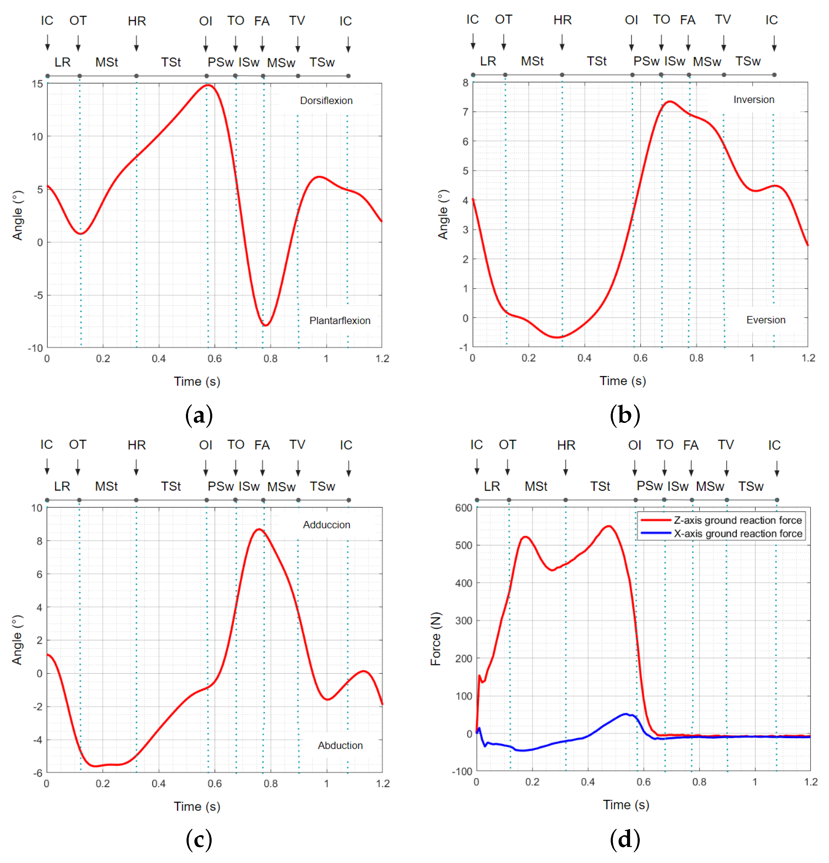
| N° | Phases | Dorsiflexion–Plantarflexion | Inversion–Eversion | Abduction–Adduction |
|---|---|---|---|---|
| 1 | Initial contact (IC) | 0 s, 5.34° | 0 s, 4.06° | 0 s, 1.13° |
| 2 | Load response (LR) | 0.011 s, 0.83° | 0.011 s, 0.28° | 0.011 s, −4.18° |
| 3 | Mid-stance (MSt) | 0.32 s, 8.07° | 0.32 s, −0.65° | 0.32 s, −4.97° |
| 4 | Terminal stance (TSt) | 0.58 s, 14.85° | 0.58 s, 3.8° | 0.58 s, −0.81° |
| 5 | Pre-swing (PSw) | 0.68 s, 5.40° | 0.68 s, 7.18° | 0.68 s, 4.38° |
| 6 | Initial swing (ISw) | 0.78 s, −7.90° | 0.78 s, 6.89° | 0.78 s, 8.43° |
| 7 | Mid-swing (MSw) | 0.9 s, 2.88° | 0.9 s, 5.85° | 0.9 s, 3.57° |
| 8 | Terminal swing (TSw) | 1.05 s, 5.31° | 1.05 s, 4.40° | 1.05 s, −0.98° |
| N° | Phases | Torque | Force |
|---|---|---|---|
| 1 | Initial contact (IC) | MATLAB: starts at 0s, torque ≈ 0 Nm. Simscape: starts at 0s, torque ≈ 0.5 Nm. Differences: not significant. | MATLAB: force starts at 0 N, and both actuators show a slight increase. Simscape: force starts at 0 N, and both actuators show a slight increase. Differences: not significant. |
| 2 | Load response (LR) | MATLAB: initial positive peak, torque ≈ 2.5 Nm. Simscape: initial positive peak, torque ≈ 2.5 Nm. Differences: not significant. | MATLAB: rapid increase in force, actuator 2 peaks around 80 N, actuator 3 around 5 N. Simscape: rapid increase in force, actuator 2 peaks around 80 N, actuator 3 around 5 N. Differences: not significant. |
| 3 | Mid-stance (MSt) | MATLAB: torque reduces to ≈2 Nm. Simscape: torque reduces to ≈2.5 Nm. Differences: not significant. | MATLAB: actuator 2 continues to increase, peaking around 150 N; actuator 3 peaks around 130 N. Simscape: actuator 2 continues to increase, peaking around 140 N; actuator 3 peaks around 110 N. Differences: not significant. |
| 4 | Terminal stance (TSt) | MATLAB: drops to ≈−2.7 Nm. Simscape: drops to ≈−2.6 Nm. Differences: not significant. | MATLAB: actuator 2 peaks around 290 N and starts to drop sharply; actuator 3 peaks around 260 N and starts to drop sharply. Simscape: actuator 2 peaks around 280 N and starts to drop sharply; actuator 3 peaks around 260 N and starts to drop sharply. Differences: not significant. |
| 5 | Pre-swing (PSw) | MATLAB: negative peak 2.7 Nm, then rises to ≈1 Nm. Simscape: negative peak 2.6 Nm, then rises to ≈1 Nm. Differences: not significant. | MATLAB: both actuators drop to around 0 N. Simscape: both actuators drop to around 0 N. Differences: not significant. |
| 6 | Initial swing (ISw) | MATLAB: stabilizes at ≈0.5 Nm. Simscape: stabilizes at ≈0.5 Nm. Differences: not significant. | MATLAB: both actuators maintain force around 0 N. Simscape: both actuators maintain force around 0 N. Differences: not significant. |
| 7 | Mid-swing (MSw) | MATLAB: stabilizes at ≈0.5 Nm. Simscape: stabilizes at ≈0.5 Nm. Differences: not significant. | MATLAB: both actuators maintain force around 0 N. Simscape: both actuators maintain force around 0 N. Differences: not significant. |
| 8 | Terminal swing (TSw) | MATLAB: stabilizes at ≈0.5 Nm. Simscape: stabilizes at ≈0.5 Nm. Differences: not significant. | MATLAB: both actuators maintain force around 0 N. Simscape: both actuators maintain force around 0 N. Differences: not significant. |
Disclaimer/Publisher’s Note: The statements, opinions and data contained in all publications are solely those of the individual author(s) and contributor(s) and not of MDPI and/or the editor(s). MDPI and/or the editor(s) disclaim responsibility for any injury to people or property resulting from any ideas, methods, instructions or products referred to in the content. |
© 2024 by the authors. Licensee MDPI, Basel, Switzerland. This article is an open access article distributed under the terms and conditions of the Creative Commons Attribution (CC BY) license (https://creativecommons.org/licenses/by/4.0/).
Share and Cite
Abarca, V.E.; Elias, D.A. Modeling and Simulation of a 2SPU-RU Parallel Mechanism for a Prosthetic Ankle with Three Degrees of Freedom. Inventions 2024, 9, 71. https://doi.org/10.3390/inventions9040071
Abarca VE, Elias DA. Modeling and Simulation of a 2SPU-RU Parallel Mechanism for a Prosthetic Ankle with Three Degrees of Freedom. Inventions. 2024; 9(4):71. https://doi.org/10.3390/inventions9040071
Chicago/Turabian StyleAbarca, Victoria E., and Dante A. Elias. 2024. "Modeling and Simulation of a 2SPU-RU Parallel Mechanism for a Prosthetic Ankle with Three Degrees of Freedom" Inventions 9, no. 4: 71. https://doi.org/10.3390/inventions9040071
APA StyleAbarca, V. E., & Elias, D. A. (2024). Modeling and Simulation of a 2SPU-RU Parallel Mechanism for a Prosthetic Ankle with Three Degrees of Freedom. Inventions, 9(4), 71. https://doi.org/10.3390/inventions9040071