
Numerical Investigation and Design Optimization of Centrifugal Water Pump with Splitter Blades Using Response Surface Method


Abstract
:1. Introduction
2. Methodology
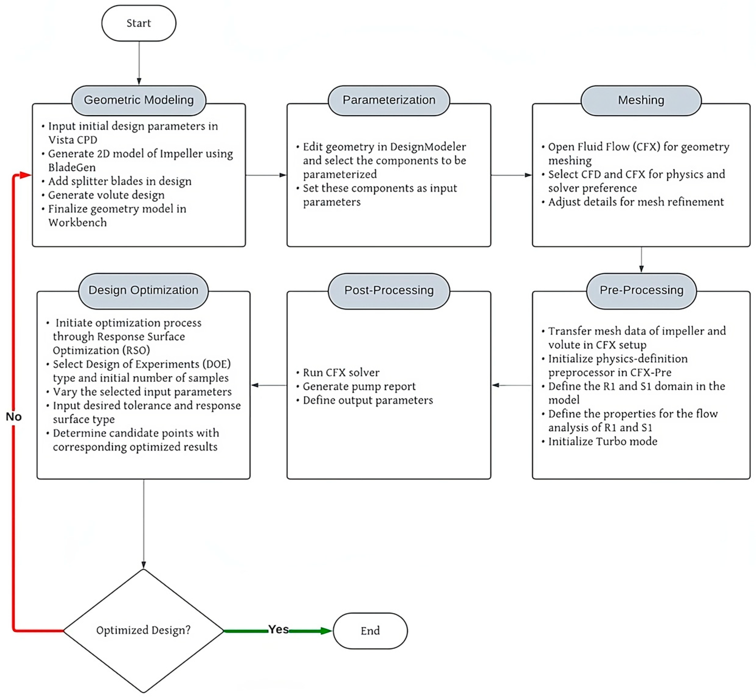
2.1. CFD Simulation Process in Centrifugal Pump Design
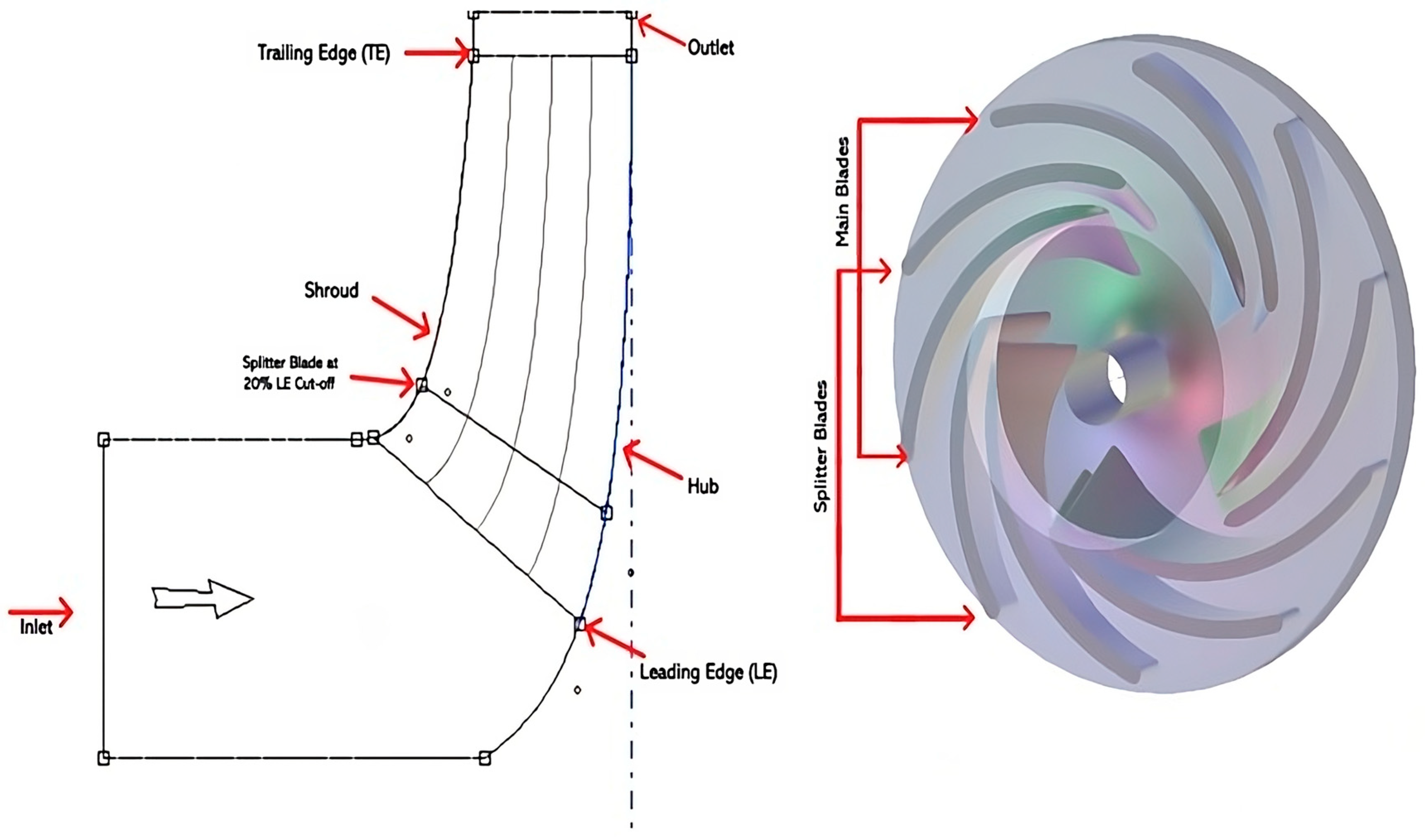
2.1.1. Geometric Modeling
2.1.2. Parameterization
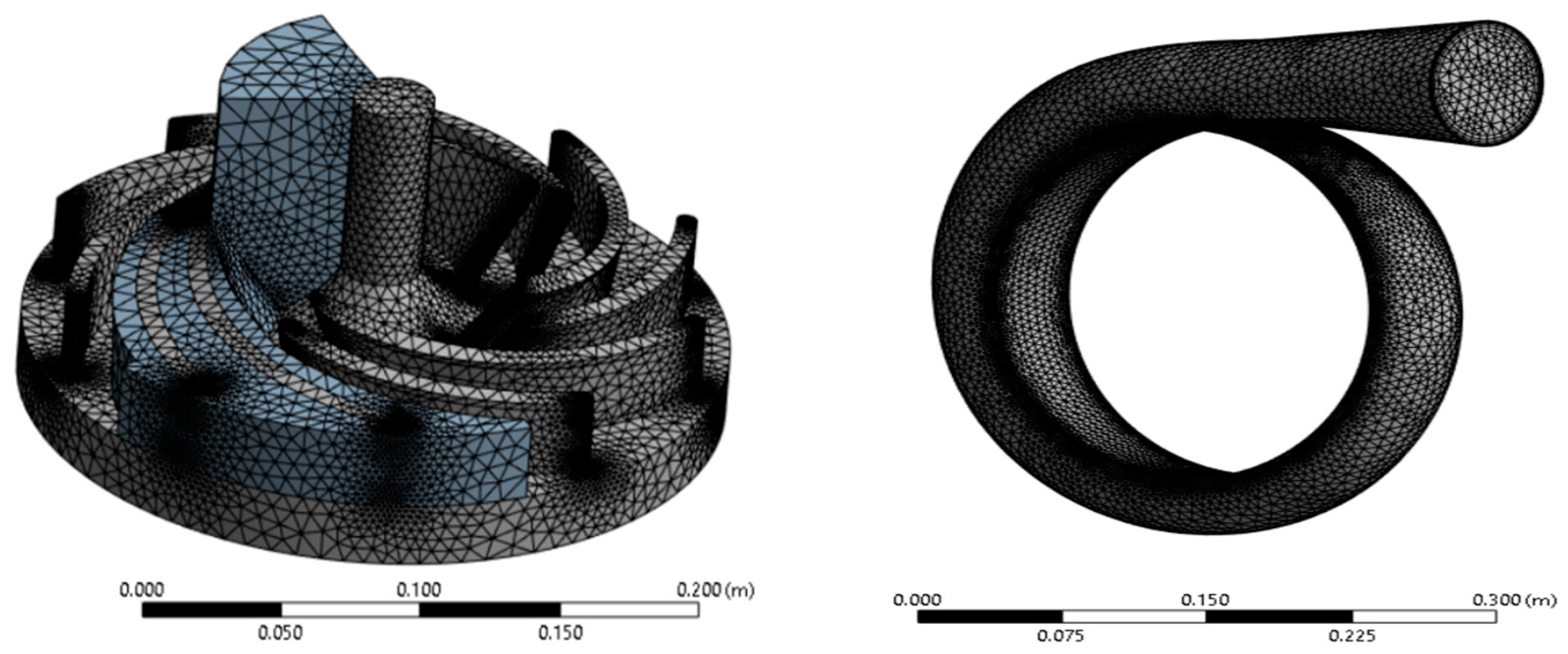
2.1.3. Meshing
2.1.4. Pre-Processing
2.1.5. Post-Processing
2.2. Optimization Process in Centrifugal Pump Design
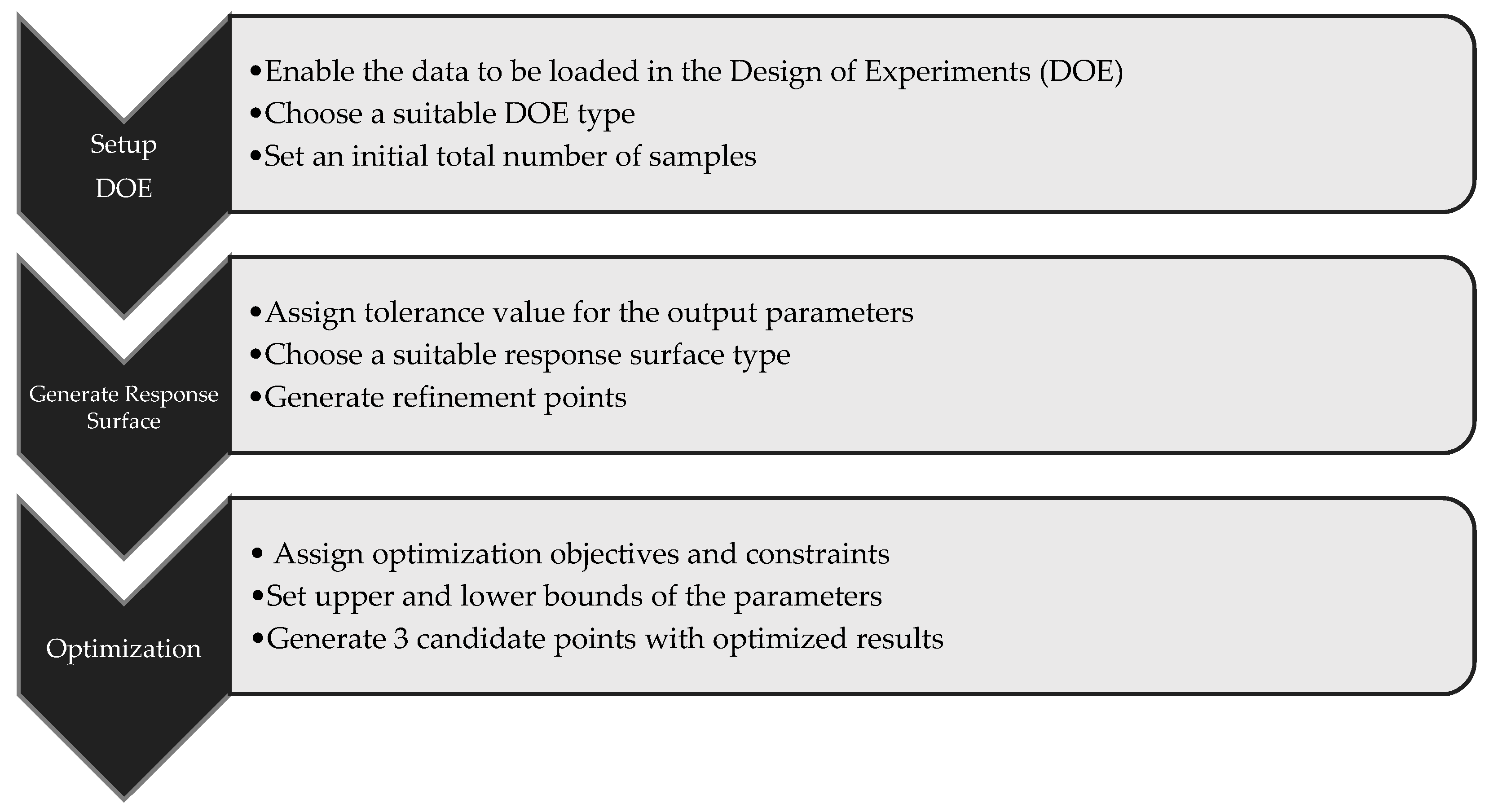
2.2.1. DOE Setup
2.2.2. Response Surface Method
2.2.3. Optimization Process
3. Results and Discussion
3.1. Baseline Design Results
3.1.1. Results Validation
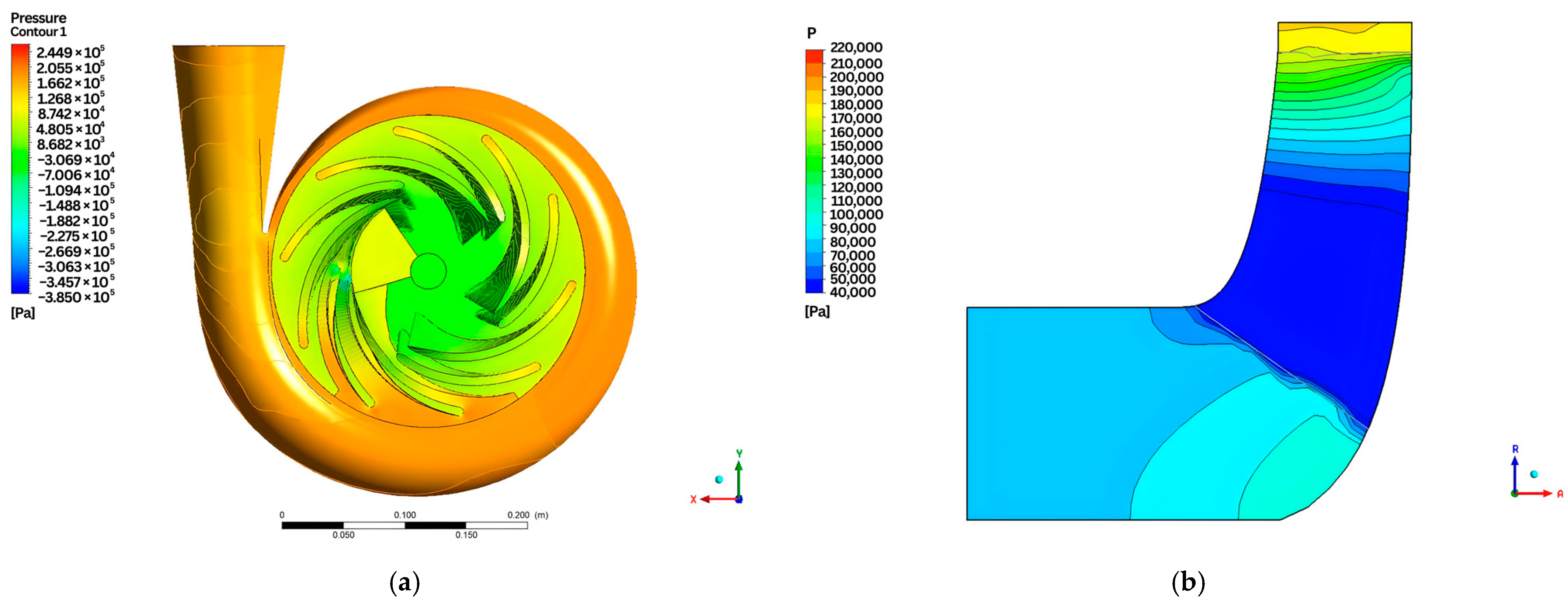
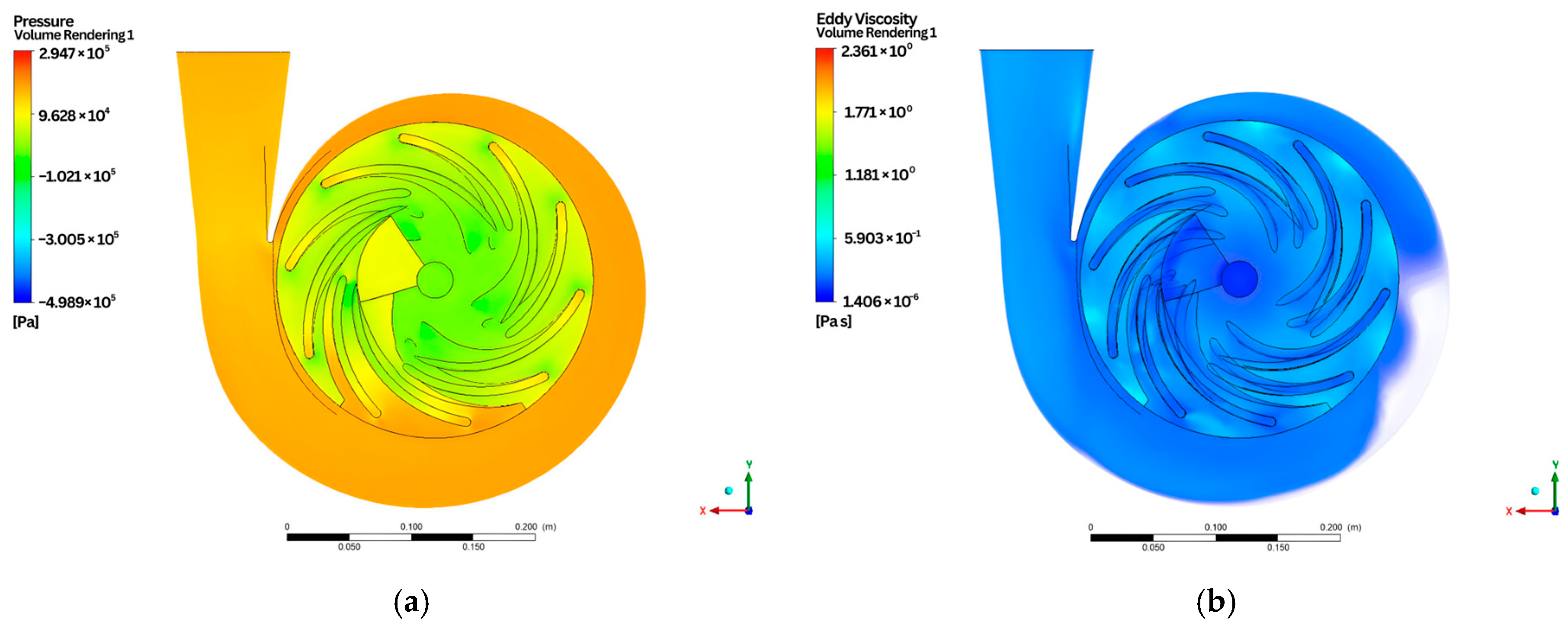
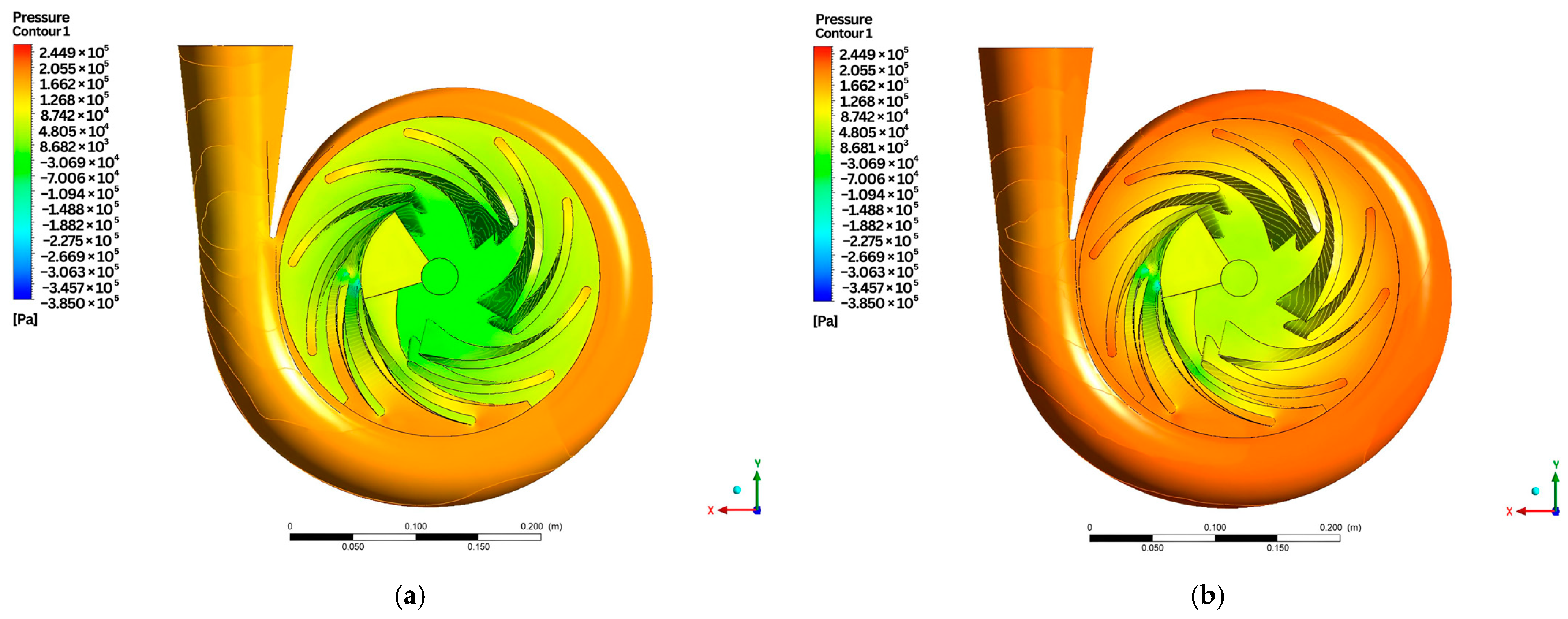
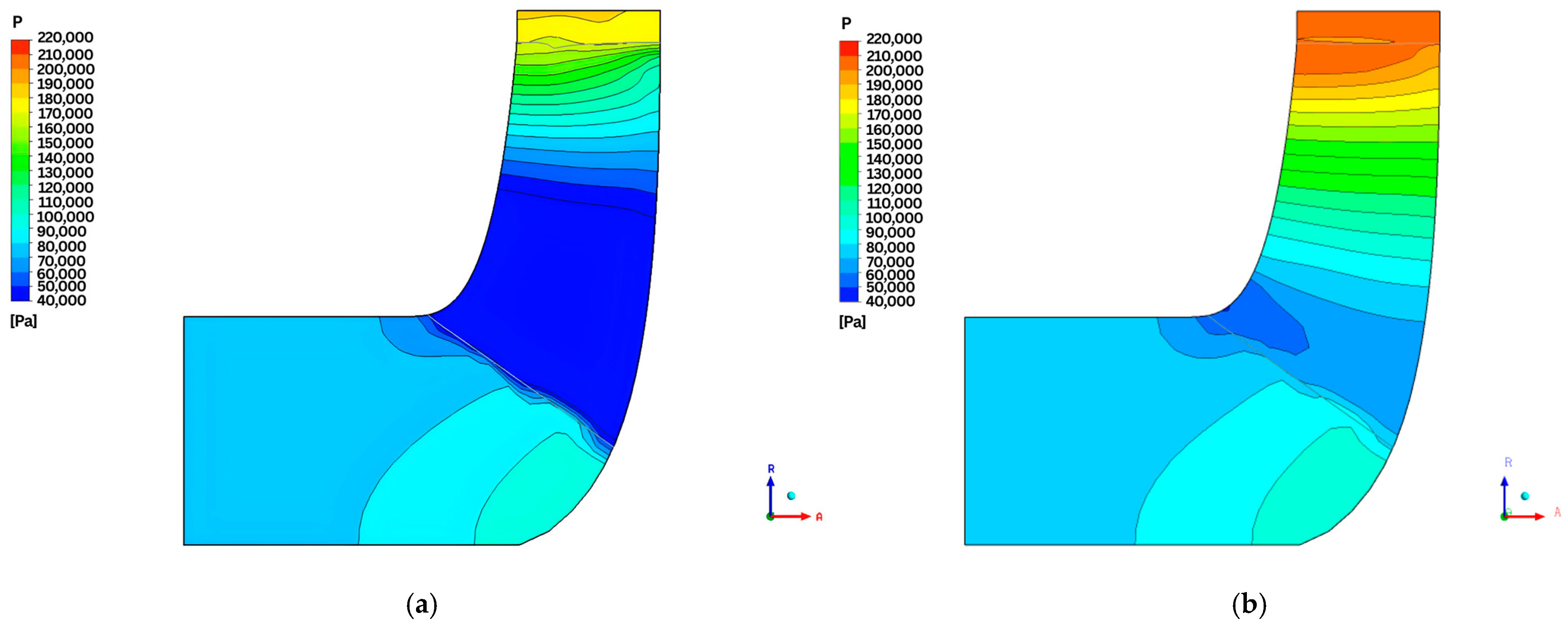
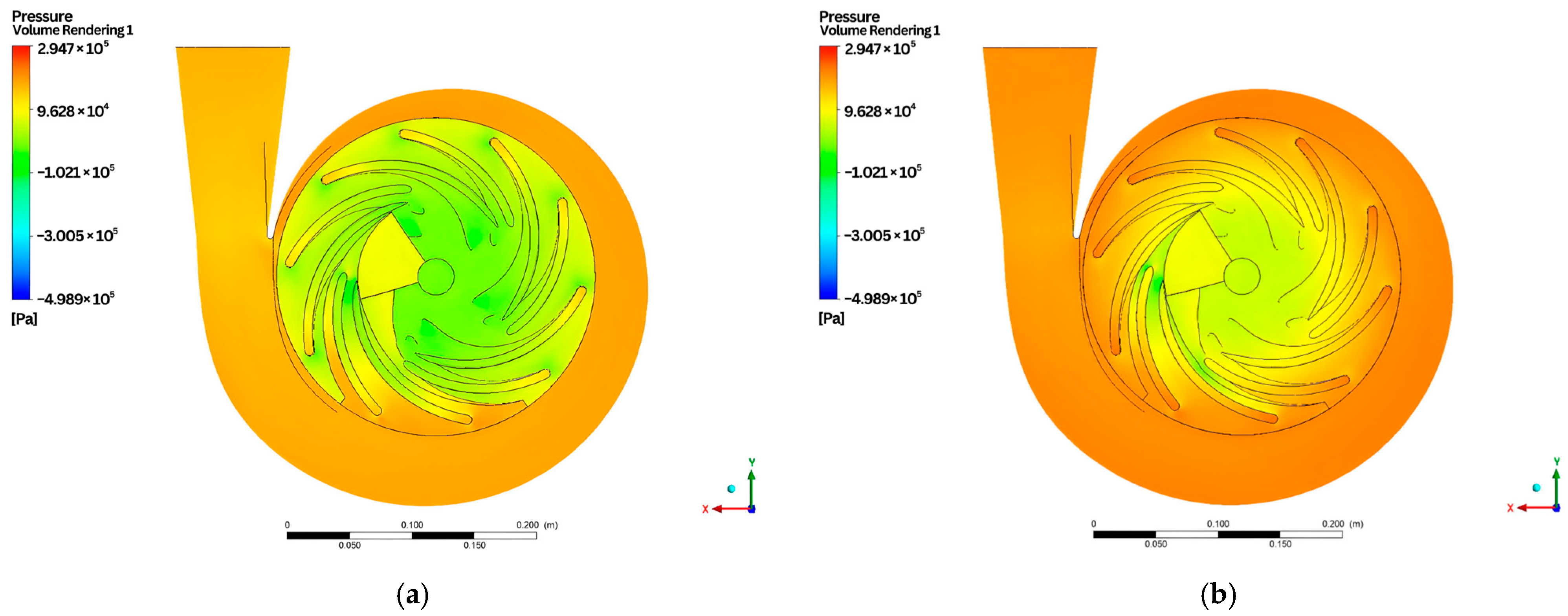
3.1.2. CFD Analysis of the Baseline Design Model
- Pressure contour plot
- 2.
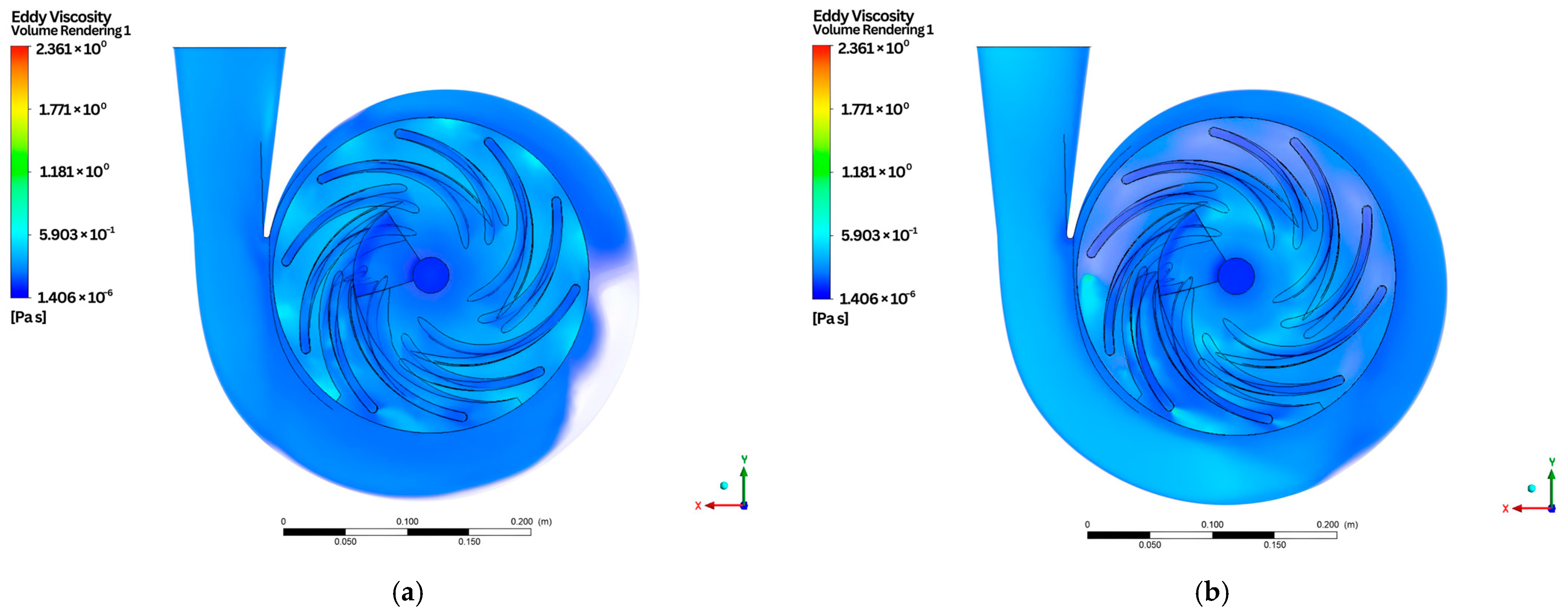
- Volume rendering of the entire domain
- 3.
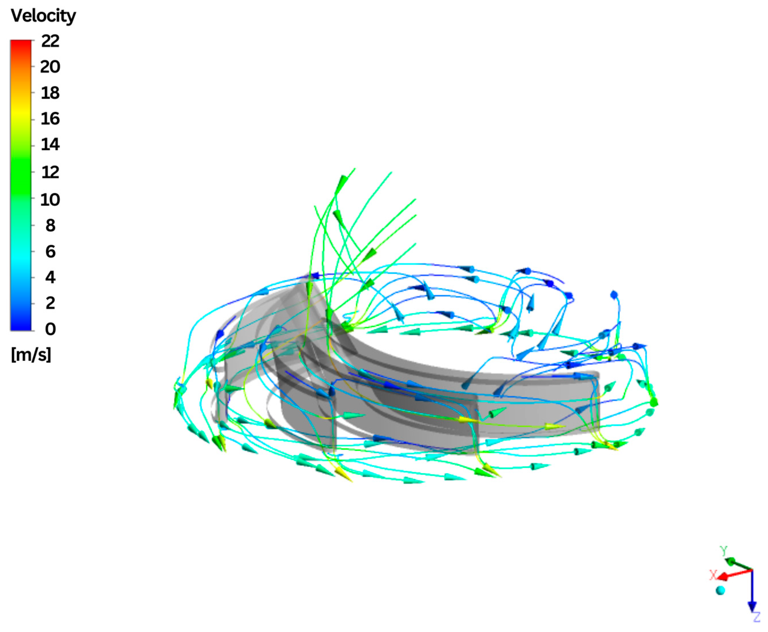
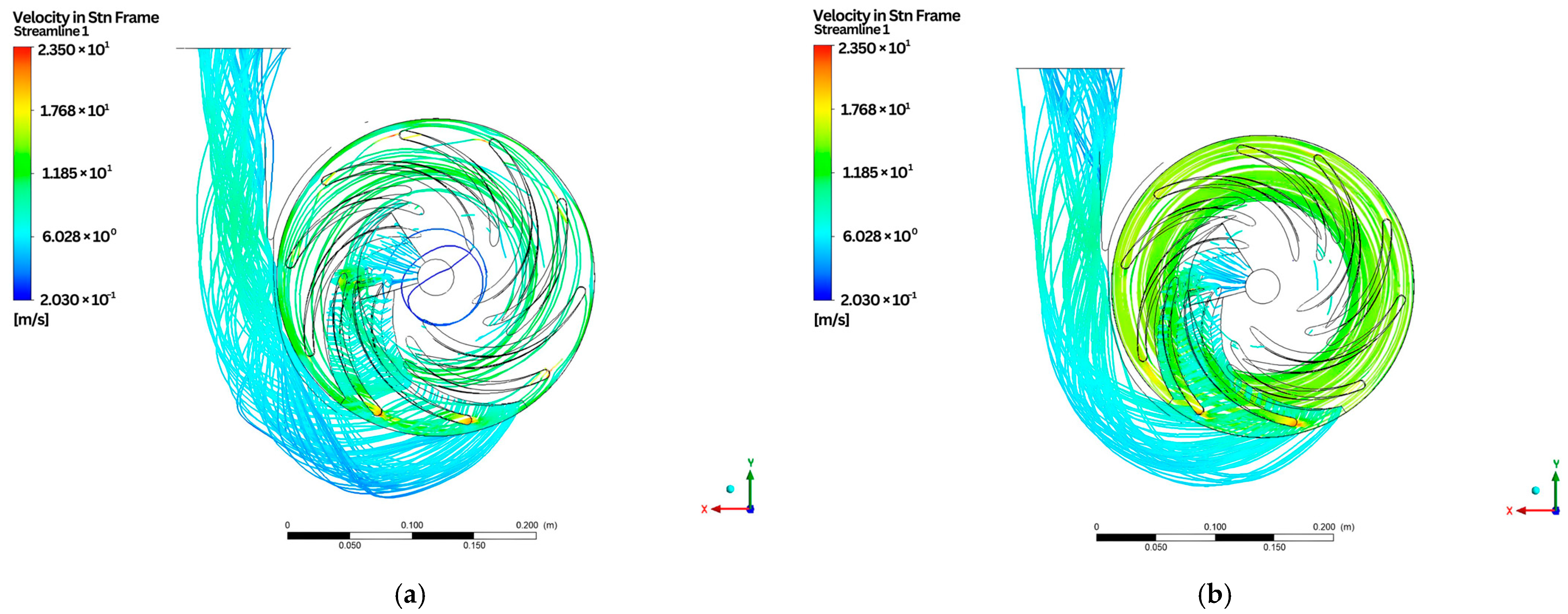
- Velocity streamline of the baseline design model
3.2. Optimization Result
3.2.1. Minimum and Maximum Generated Response
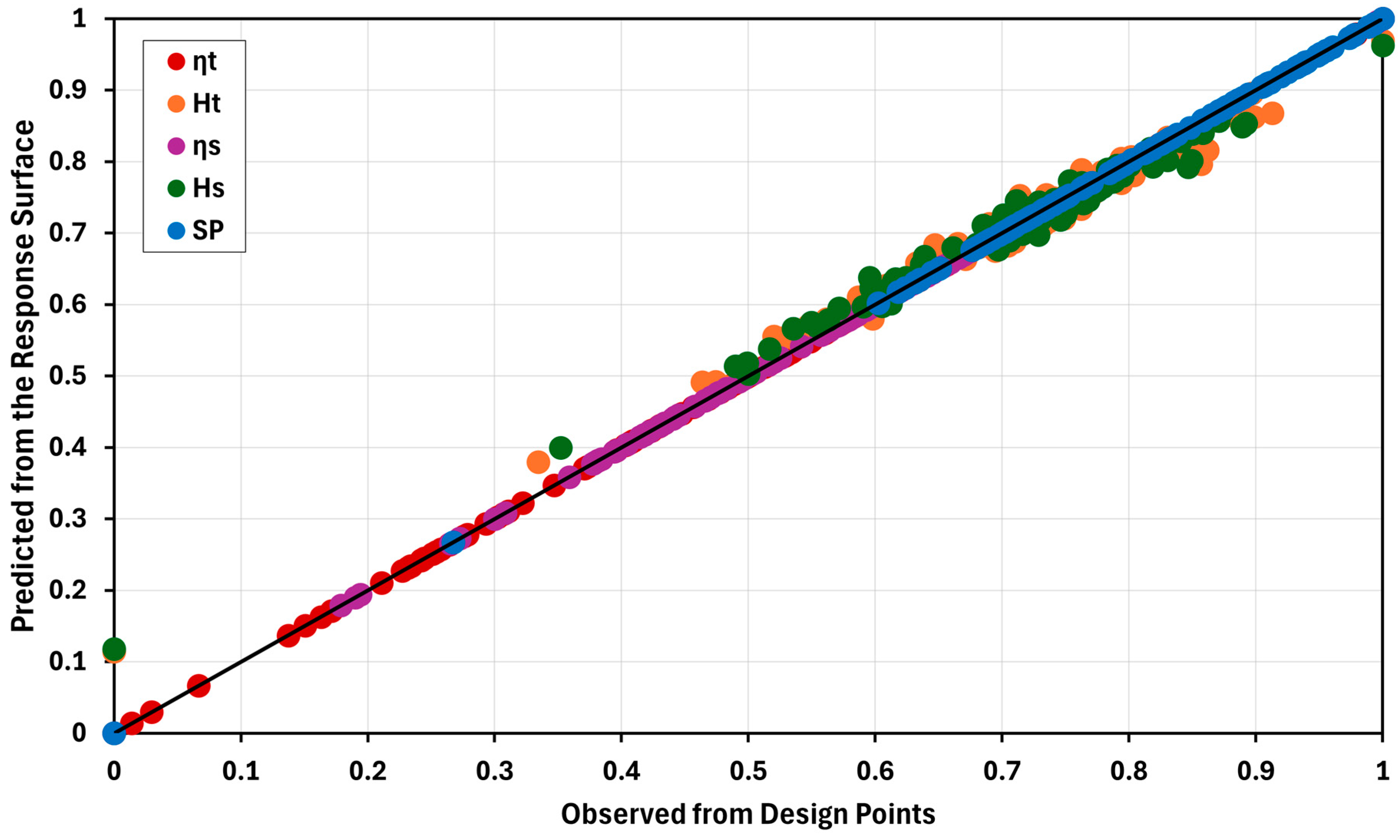
3.2.2. Goodness of Fit (GOF) Chart
3.2.3. Sensitivity Analysis
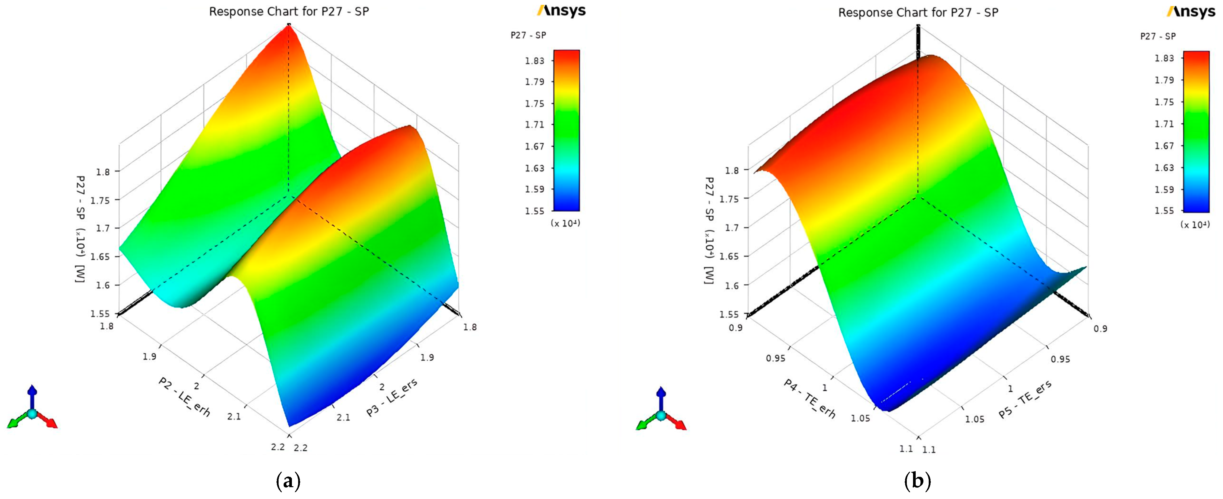
3.2.4. Response Surface Charts
- 2.
- and
- 3.
- Splitter blades’ , , , and
- Total Efficiency ()
- Total Head ()
- Static Efficiency ()
- Static Head ()
- Shaft Power ()
3.2.5. Optimal Candidate Points
3.3. Comparison of Results
4. Conclusions
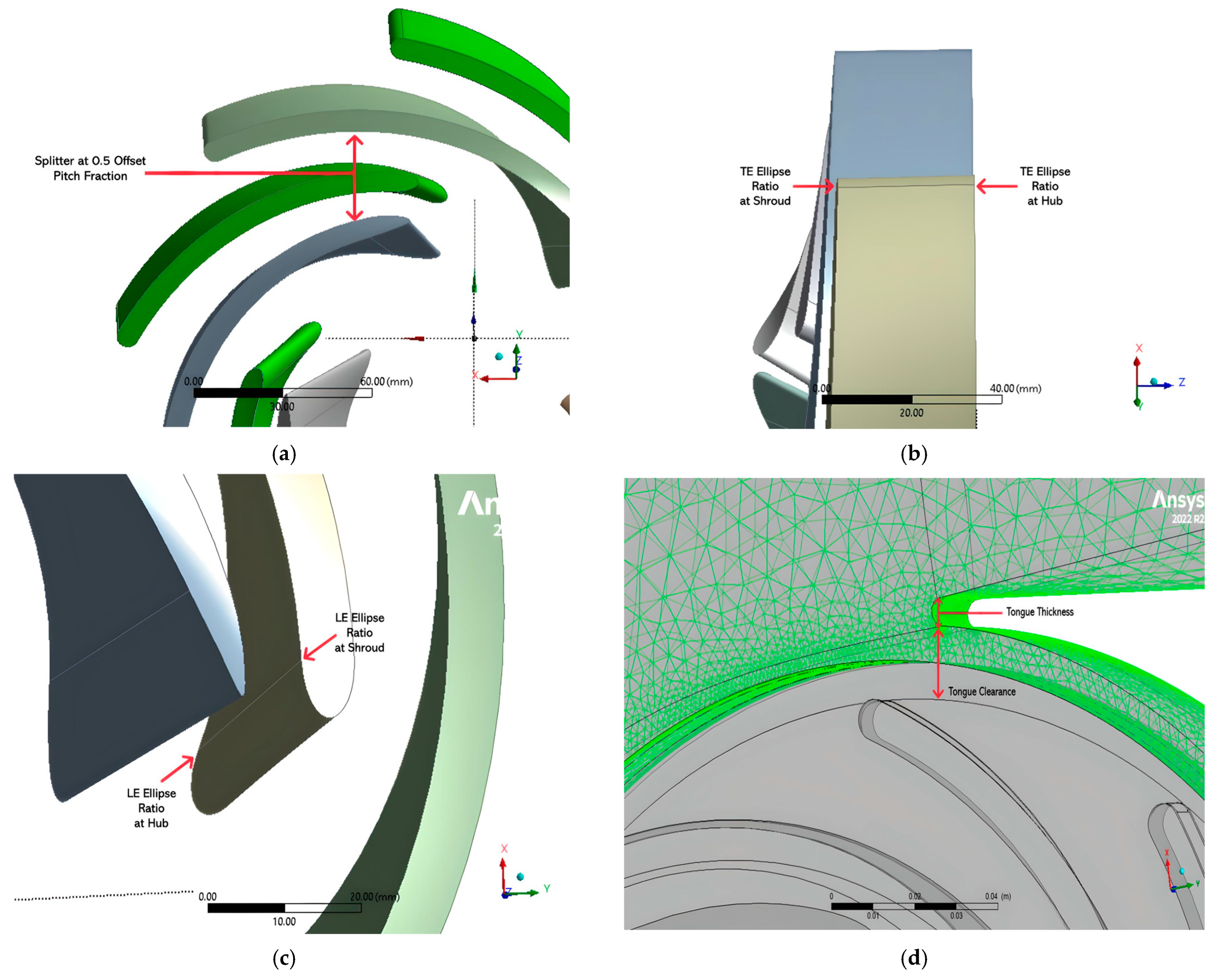
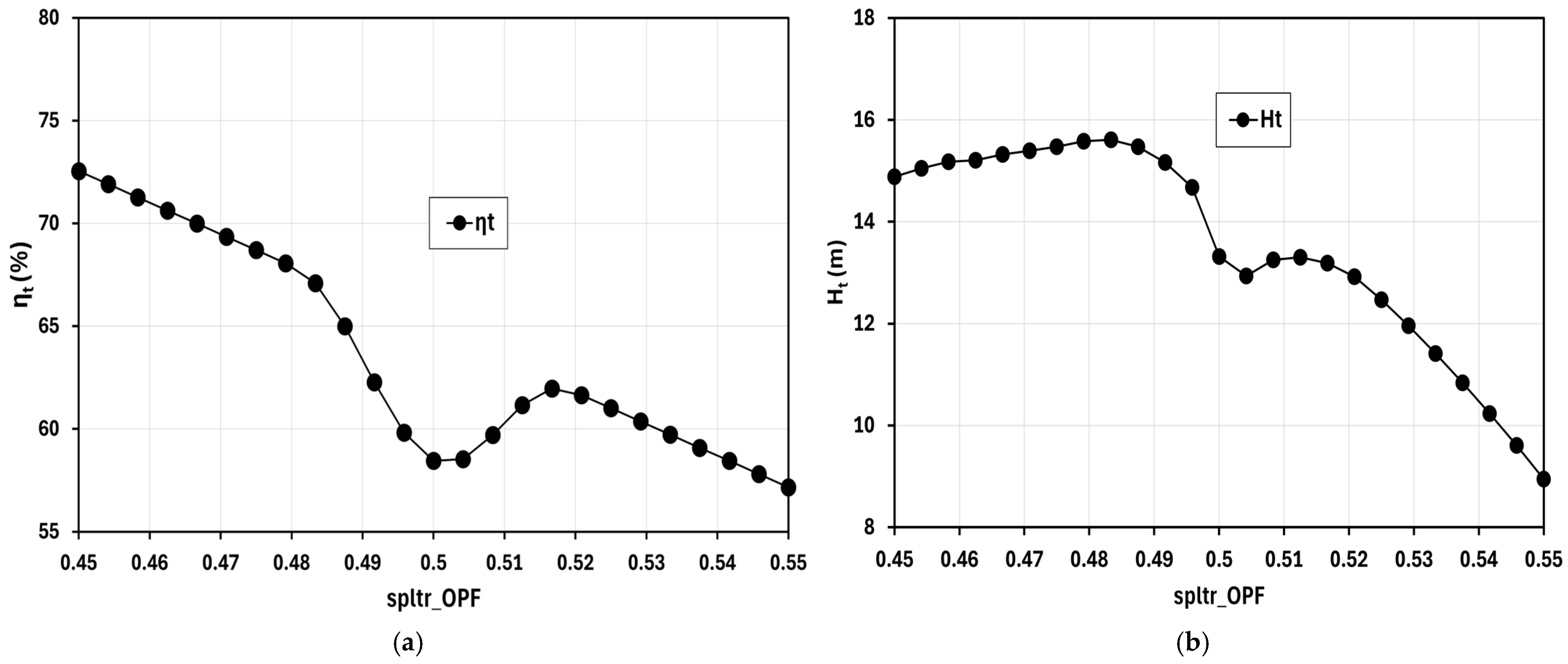
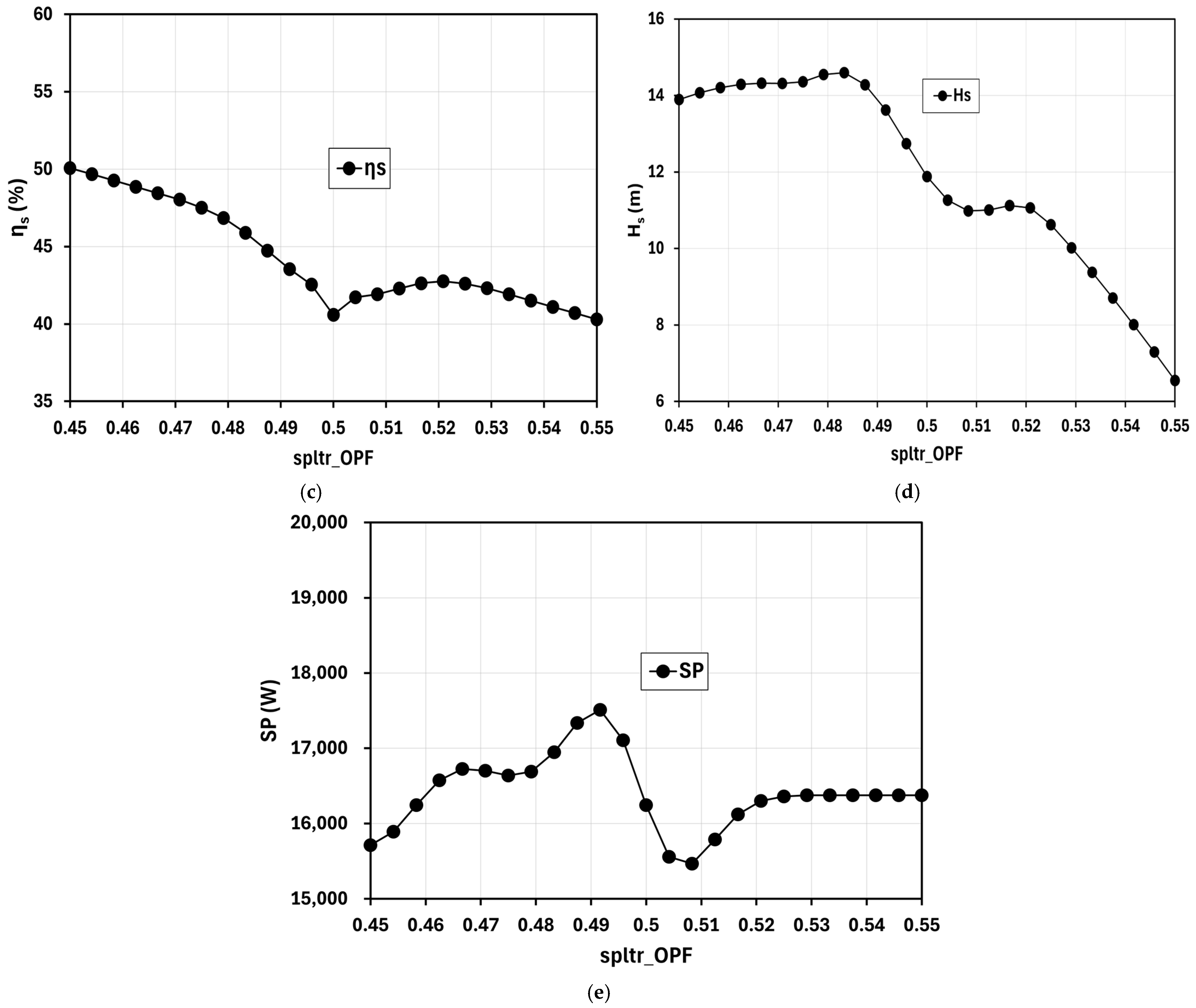
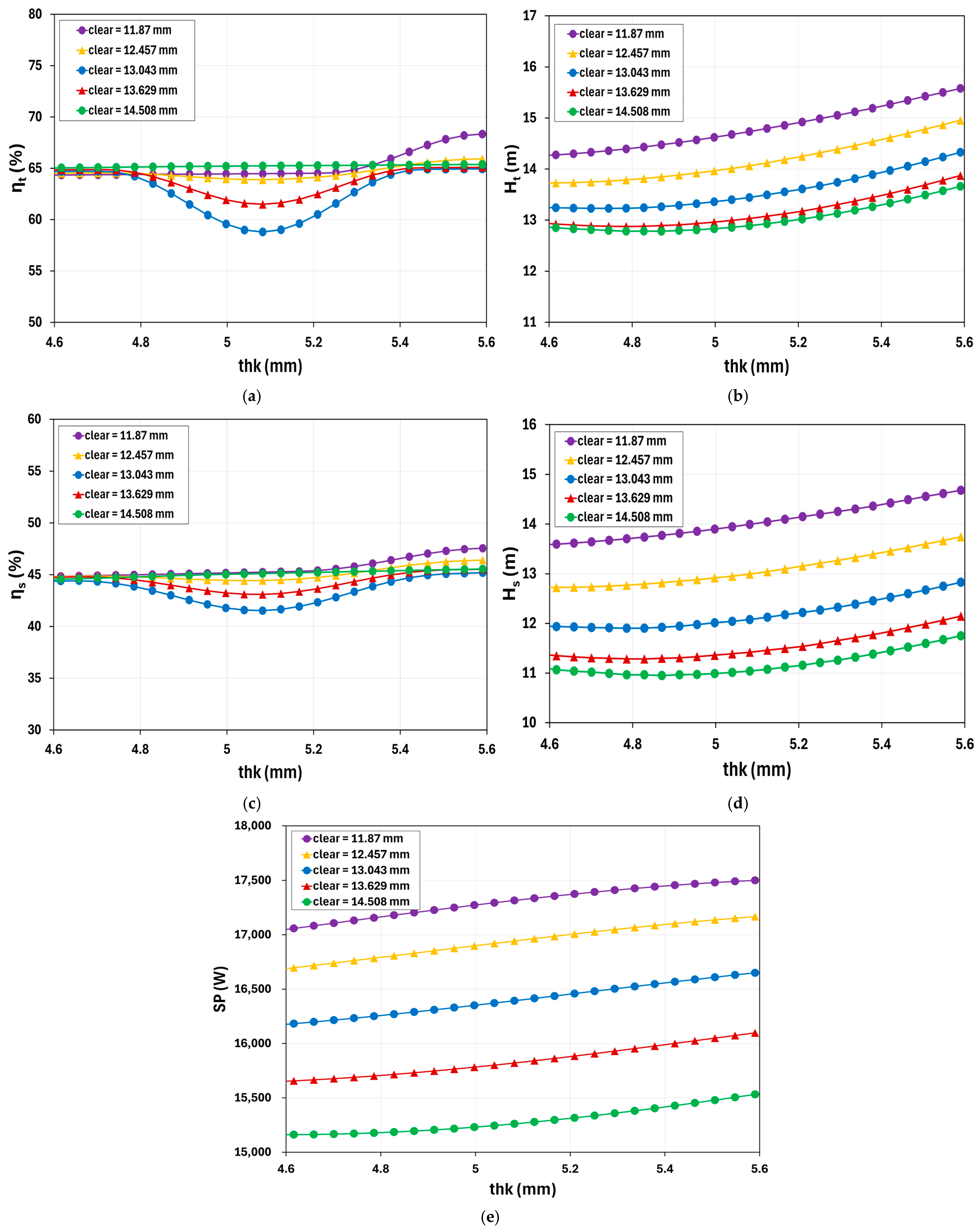
- The result established that should maintain a value of less than 0.5. As per the result of the optimized design, the should be at a value of 0.45 as this value improves the , , , and while also minimizing the . This value also coincides with the graphs presented in Figure 12.
- Based on the analysis conducted on the graphs presented in Figure 13, the performance of the pump can be improved when the increases while maintaining the at a minimum level. This analysis shows to be coherent with the results of the and provided in Table 18. In the table, the value of the increases from 5.082 mm to 5.579 mm while having a reduced value for the from 13.189 mm to 12.994 mm. This explains the significance of the optimization results. Having these modifications for the volute tongue improves the dynamics between the impeller and the volute, enhancing the pump’s hydraulic efficiency. This finding highlights the significance of the impeller–volute interaction. Hence, it can be concluded that the volute of the pump should also be considered when modifying the impeller.
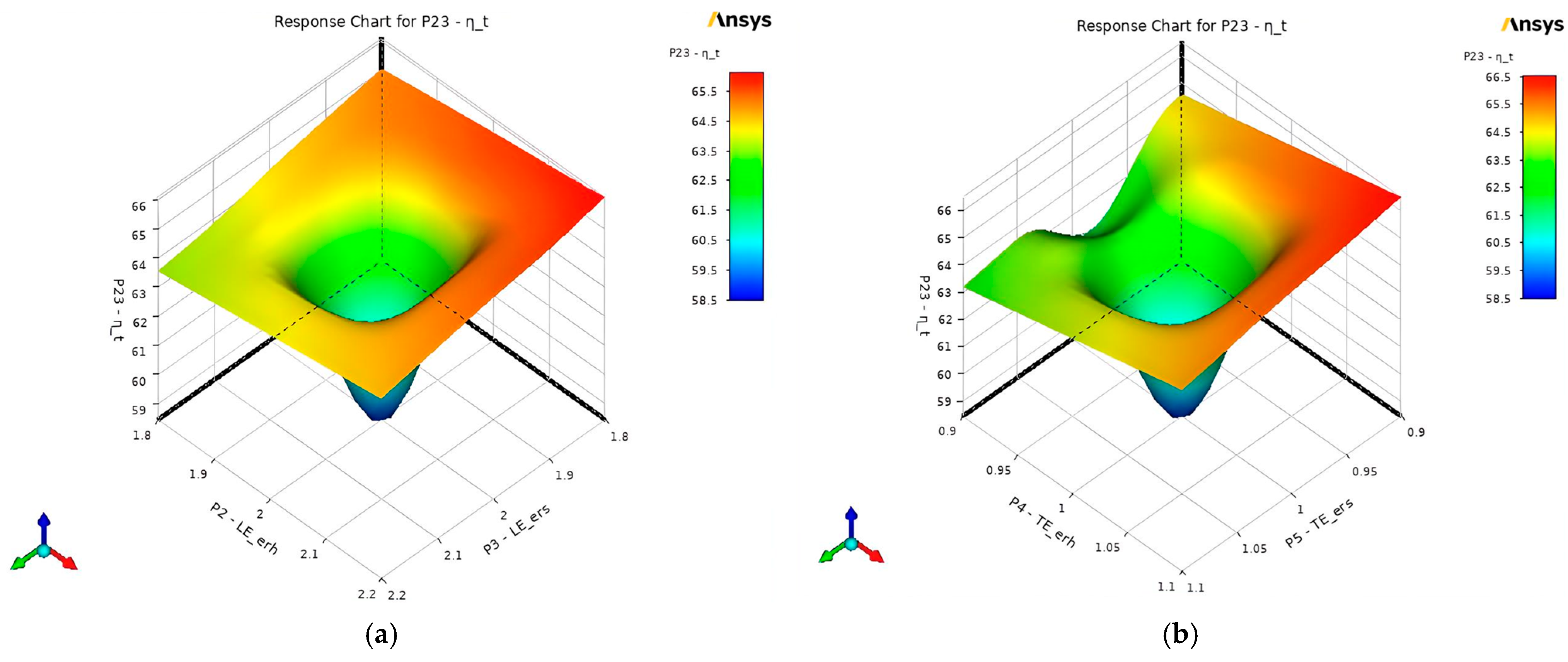
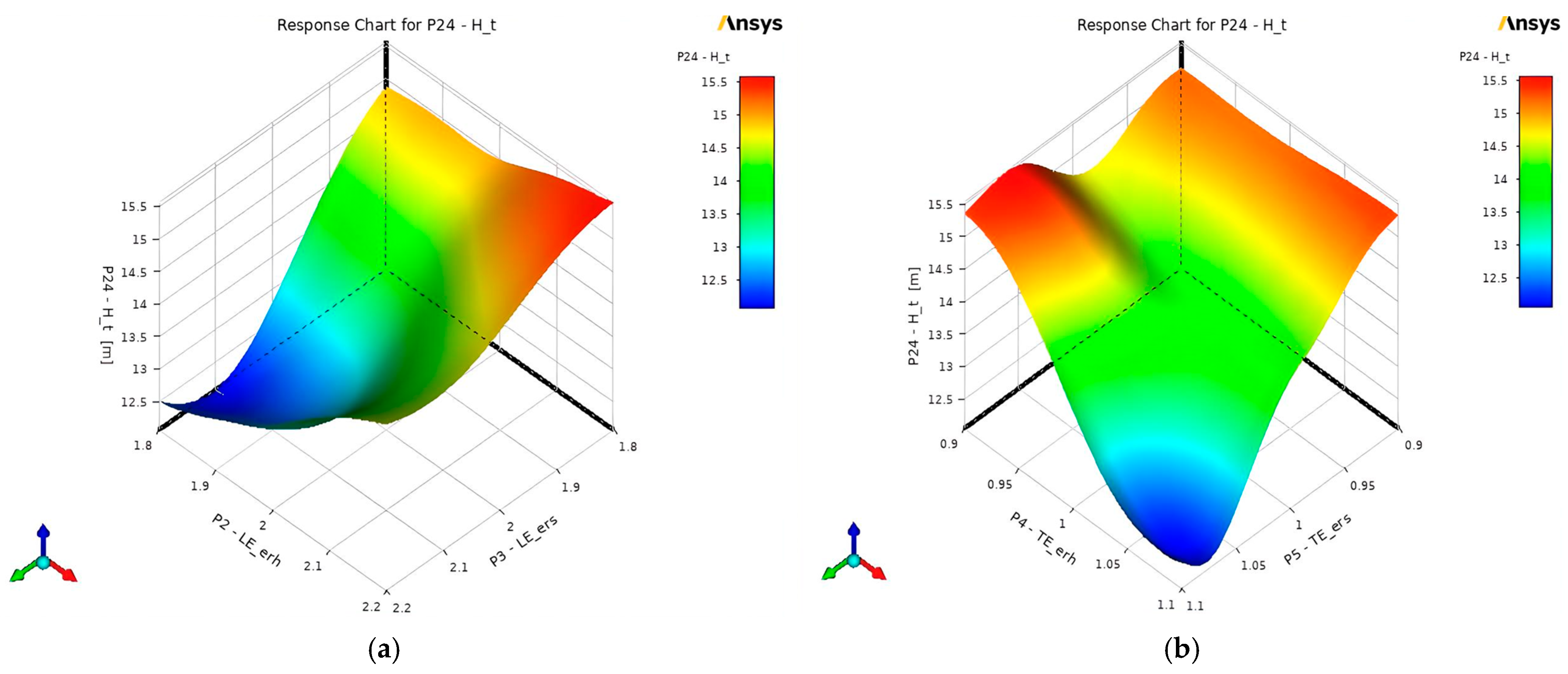
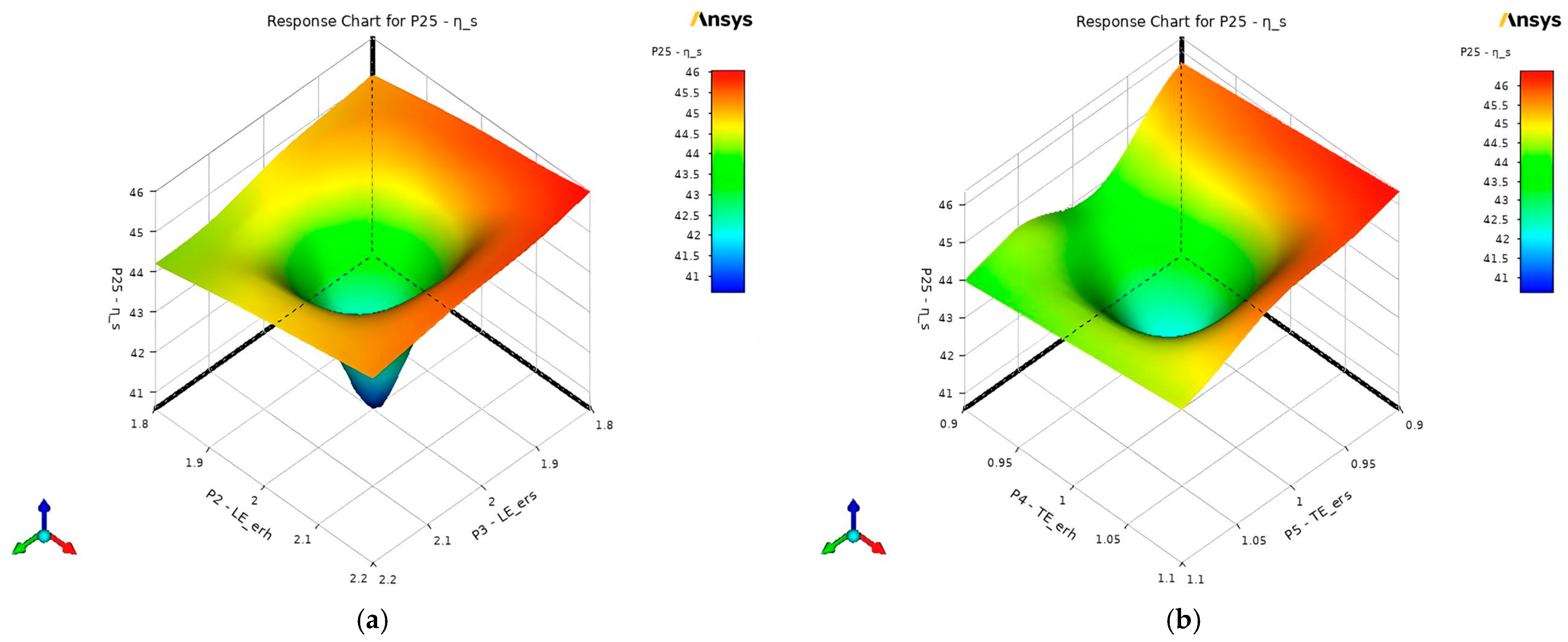
- For the LE and TE ellipse ratios, improvements in the performance of the pump, such as the , , , and were achieved when both and increased and both the and decreased from their initial values of 2 and 1 for LE and TE, respectively.
- Reducing the requires different LE and TE configurations. In LE, setting the and to a value greater than their initial value of 2 will help minimize the power required by the shaft. On the other hand, the should maintain a value closer to 1.06, and there should be an increasing value of the that is greater than 1 to minimize the .
- Configuring the LE and TE of the splitter blades to reduce the to its full extent may compromise the efficiencies and heads due to the differences in their required configurations. Therefore, finding the perfect balance between these parameters is essential to achieve a desirable pump performance with conflicting parametric objectives and constraints.
- The optimal design of the study resulted in 27.35%, 15.70%, 28.18%, and 16.67% improvement in , , , and , respectively, while achieving an 8.36% decrease in .
- Although this study was able to obtain improvement with the design of centrifugal water pump, the need for actual implementation of this study remains to be a possibility for further research. Researchers may consider applying the findings of this study to an actual setup where changes in temperature and sudden drops in pressure may become a challenging aspect for future work.
5. Recommendation
Author Contributions
Funding
Data Availability Statement
Conflicts of Interest
Nomenclature
| volute tongue clearance | |
| gravity, 9.81 m/s2 | |
| static head | |
| total head | |
| total-static head, 8.069 m | |
| turbulence kinetic energy | |
| leading edge ellipse ratio at hub | |
| leading edge ellipse ratio at shroud | |
| static pressure | |
| volume flow rate, 0.084 m3/s | |
| shaft/input power | |
| splitter blades’ offset pitch fraction | |
| trailing edge ellipse ratio at hub | |
| trailing edge ellipse ratio at shroud | |
| volute tongue thickness | |
| mean fluid speed | |
| flow velocity | |
| kinematic viscosity | |
| density of fluid | |
| density of water, 997 kg/m3 | |
| static efficiency | |
| total efficiency | |
| specific dissipation rate |
References
- Nguyen, V.T.T.; Vo, T.M.N. Centrifugal Pump Design: An Optimization. Eurasia Proc. Sci. Technol. Eng. Math. 2022, 17, 136–151. [Google Scholar] [CrossRef]
- Zhang, L.; Wang, X.; Wu, P.; Huang, B.; Wu, D. Optimization of a Centrifugal Pump to Improve Hydraulic Efficiency and Reduce Hydro-Induced Vibration. Energy 2023, 268, 126677. [Google Scholar] [CrossRef]
- Zhang, W.; An, L.; Li, X.; Chen, F.; Sun, L.; Wang, X.; Cai, J. Adjustment Method and Energy Consumption of Centrifugal Pump Based on Intelligent Optimization Algorithm. Energy Rep. 2022, 8, 12272–12281. [Google Scholar] [CrossRef]
- Arun Shankar, V.K.; Umashankar, S.; Paramasivam, S.; Hanigovszki, N. A Comprehensive Review on Energy Efficiency Enhancement Initiatives in Centrifugal Pumping System. Appl. Energy 2016, 181, 495–513. [Google Scholar] [CrossRef]
- Chen, W.; Li, Y.; Liu, Z.; Hong, Y. Understanding of Energy Conversion and Losses in a Centrifugal Pump Impeller. Energy 2023, 263, 125787. [Google Scholar] [CrossRef]
- Shojaeefard, M.H.; Saremian, S. Effects of Impeller Geometry Modification on Performance of Pump as Turbine in the Urban Water Distribution Network. Energy 2022, 255, 124550. [Google Scholar] [CrossRef]
- Shojaeefard, M.H.; Saremian, S. Analyzing the Impact of Blade Geometrical Parameters on Energy Recovery and Efficiency of Centrifugal Pump as Turbine Installed in the Pressure-Reducing Station. Energy 2024, 289, 130004. [Google Scholar] [CrossRef]
- Wu, C.; Pu, K.; Shi, P.; Wu, P.; Huang, B.; Wu, D. Blade Redesign Based on Secondary Flow Suppression to Improve the Dynamic Performance of a Centrifugal Pump. J. Sound Vib. 2023, 554, 117689. [Google Scholar] [CrossRef]
- Siddique, M.H.; Samad, A.; Hossain, S. Centrifugal Pump Performance Enhancement: Effect of Splitter Blade and Optimization. Proc. Inst. Mech. Eng. Part. A 2021, 236, 391–402. [Google Scholar] [CrossRef]
- Gao, B.; Zhang, N.; Li, Z.; Ni, D.; Yang, M.G. Influence of the Blade Trailing Edge Profile on the Performance and Unsteady Pressure Pulsations in a Low Specific Speed Centrifugal Pump. J. Fluids Eng. Trans. ASME 2016, 138, 051106. [Google Scholar] [CrossRef]
- Tao, R.; Xiao, R.; Wang, Z. Influence of Blade Leading-Edge Shape on Cavitation in a Centrifugal Pump Impeller. Energies 2018, 11, 2588. [Google Scholar] [CrossRef]
- Fernández Oro, J.M.; Barrio Perotti, R.; Galdo Vega, M.; González, J. Effect of the Radial Gap Size on the Deterministic Flow in a Centrifugal Pump Due to Impeller-Tongue Interactions. Energy 2023, 278, 127820. [Google Scholar] [CrossRef]
- Shah, S.R.; Jain, S.V.; Patel, R.N.; Lakhera, V.J. CFD for Centrifugal Pumps: A Review of the State-of-the-Art. Procedia Eng. 2013, 51, 715–720. [Google Scholar] [CrossRef]
- Wu, T.X.; Wu, D.H.; Gao, S.Y.; Song, Y.; Ren, Y.; Mou, J.G. Multi-Objective Optimization and Loss Analysis of Multistage Centrifugal Pumps. Energy 2023, 284, 128638. [Google Scholar] [CrossRef]
- Baker, C.; Johnson, T.; Flynn, D.; Hemida, H.; Quinn, A.; Soper, D.; Sterling, M. Fluid Mechanics Concepts. In Train Aerodynamics; Butterworth-Heinemann: Oxford, UK, 2019; pp. 17–33. [Google Scholar] [CrossRef]
- Palanikumar, K. Introductory Chapter: Response Surface Methodology in Engineering Science. In Response Surface Methodology in Engineering Science; IntechOpen: London, UK, 2021. [Google Scholar] [CrossRef]
- Şengöz, N.G. Practicing Response Surface Designs in Textile Engineering: Yarn Breaking Strength Exercise. In Response Surface Methodology in Engineering Science; IntechOpen: London, UK, 2021. [Google Scholar] [CrossRef]
- Safikhani, H.; Khalkhali, A.; Farajpoor, M. Pareto Based Multi-Objective Optimization of Centrifugal Pumps Using CFD, Neural Networks and Genetic Algorithms. Eng. Appl. Comput. Fluid Mech. 2011, 5, 37–48. [Google Scholar] [CrossRef]
- Lu, C.; Fuh, J.Y.H.; Wong, Y.S. Advanced Assembly Planning Approach Using a Multi-Objective Genetic Algorithm. In Collaborative Product Assembly Design and Assembly Planning; Woodhead Publishing: Sawston, UK, 2011; pp. 107–146. [Google Scholar] [CrossRef]
- Nikjoofar, A.; Zarghami, M. Water Distribution Networks Designing by the Multiobjective Genetic Algorithm and Game Theory. In Metaheuristics in Water, Geotechnical and Transport Engineering; Elsevier: Amsterdam, The Netherlands, 2013; pp. 99–119. [Google Scholar] [CrossRef]
- Brentan, B.; Mota, F.; Menapace, A.; Zanfei, A.; Meirelles, G. Optimizing Pump Operations in Water Distribution Networks: Balancing Energy Efficiency, Water Quality and Operational Constraints. J. Water Process Eng. 2024, 63, 105374. [Google Scholar] [CrossRef]
- Alawadhi, K.; Alzuwayer, B.; Mohammad, T.A.; Buhemdi, M.H. Design and Optimization of a Centrifugal Pump for Slurry Transport Using the Response Surface Method. Machines 2021, 9, 60. [Google Scholar] [CrossRef]
- Gölcü, M.; Usta, N.; Pancar, Y. Effects of Splitter Blades on Deep Well Pump Performance. J. Energy Resour. Technol. 2007, 129, 169–176. [Google Scholar] [CrossRef]
- Chen, B.; Qian, Y. Effects of Blade Suction Side Modification on Internal Flow Characteristics and Hydraulic Performance in a PIV Experimental Centrifugal Pump. Processes 2022, 10, 2479. [Google Scholar] [CrossRef]
- Zhang, N.; Liu, X.; Gao, B.; Wang, X.; Xia, B. Effects of Modifying the Blade Trailing Edge Profile on Unsteady Pressure Pulsations and Flow Structures in a Centrifugal Pump. Int. J. Heat Fluid Flow 2019, 75, 227–238. [Google Scholar] [CrossRef]
- Alemi, H.; Nourbakhsh, S.A.; Raisee, M.; Najafi, A.F. Effect of the Volute Tongue Profile on the Performance of a Low Specific Speed Centrifugal Pump. Proc. Inst. Mech. Eng. Part A J. Power Energy 2015, 229, 210–220. [Google Scholar] [CrossRef]
- Tu, J.; Yeoh, G.H.; Liu, C.; Tao, Y. CFD Mesh Generation—A Practical Guideline. In Computational Fluid Dynamics; Butterworth-Heinemann: Oxford, UK, 2024; pp. 123–151. [Google Scholar] [CrossRef]
- Hu, P.; Li, Y.; Cai, C.S.; Liao, H.; Xu, G.J. Numerical Simulation of the Neutral Equilibrium Atmospheric Boundary Layer Using the SST K-ω Turbulence Model. Wind Struct. Int. J. 2013, 17, 87–105. [Google Scholar] [CrossRef]
- Menter, F.R. Two-Equation Eddy-Viscosity Turbulence Models for Engineering Applications. AIAA J. 1994, 32, 1598–1605. [Google Scholar] [CrossRef]
- Pagayona, E.; Honra, J. Multi-Criteria Response Surface Optimization of Centrifugal Pump Performance Using CFD for Wastewater Application. Modelling 2024, 5, 673–693. [Google Scholar] [CrossRef]
- Wang, M.; Zhang, Y.; Lu, Y.; Wan, X.; Xu, B.; Yu, L. Comparison of Multi-Objective Genetic Algorithms for Optimization of Cascade Reservoir Systems. J. Water Clim. Change 2022, 13, 4069–4086. [Google Scholar] [CrossRef]
- Karamian, F.; Mirakzadeh, A.A.; Azari, A. Application of Multi-Objective Genetic Algorithm for Optimal Combination of Resources to Achieve Sustainable Agriculture Based on the Water-Energy-Food Nexus Framework. Sci. Total Environ. 2023, 860, 160419. [Google Scholar] [CrossRef] [PubMed]
- Morabito, A.; Vagnoni, E.; Di Matteo, M.; Hendrick, P. Numerical Investigation on the Volute Cutwater for Pumps Running in Turbine Mode. Renew Energy 2021, 175, 807–824. [Google Scholar] [CrossRef]
- Zakeralhoseini, S.; Schiffmann, J. The Influence of Splitter Blades and Meridional Profiles on the Performance of Small-Scale Turbopumps for ORC Applications; Analysis, Neural Network Modeling and Optimization. Therm. Sci. Eng. Prog. 2023, 39, 101734. [Google Scholar] [CrossRef]


| Input Parameter | Unit | Value |
|---|---|---|
| Rotational Speed | RPM | 1600 |
| Volume Flow Rate | m3/h | 120 |
| Density | kg/m3 | 1000 |
| Head Rise | m | 20 |
| Inlet Flow Angle | degrees | 90 |
| Merid Velocity Ratio | - | 1.1 |
| Number of Vanes | - | 5 |
| Impeller Specification | Unit | Value |
|---|---|---|
| Shaft Diameter | mm | 19.611 |
| Hub Eye Diameter | mm | 29.416 |
| Eye Diameter | mm | 125.75 |
| Vane Thickness | mm | 7.260 |
| Tip Diameter | mm | 242.01 |
| Tip Width | mm | 30.215 |
| Number of Main Blade | - | 5 |
| Number of Splitter Blade | - | 5 |
| Volute Specification | Unit | Value |
|---|---|---|
| Inlet Width | mm | 60.431 |
| Base Circle Radius | mm | 134.19 |
| Tongue Clearance | mm | 13.189 |
| Tongue Thickness | mm | 5.082 |
| Diffuser Length | mm | 151.79 |
| Diffuser Cone Angle | degree | 7 |
| Diffuser Outlet Hydraulic Diameter | mm | 91.868 |
| Diffuser Outlet Height | mm | 91.868 |
| Parameter | Unit | Value |
|---|---|---|
| - | 0.5 | |
| - | 2 | |
| - | 2 | |
| - | 1 | |
| - | 1 | |
| mm | 13.189 | |
| mm | 5.082 |
| Impeller | Volute | (m) | (%) Change | ||||
|---|---|---|---|---|---|---|---|
| Growth Rate | Nodes | Elements | Growth Rate | Nodes | Elements | ||
| 1.1 | 759,200 | 4,145,000 | 1.2 | 89,559 | 271,970 | 18.812 | 0 |
| 1.2 | 251,260 | 1,277,300 | 1.3 | 75,273 | 212,850 | 18.868 | 0.297 |
| 1.3 | 194,380 | 946,550 | 1.4 | 68,536 | 186,750 | 18.693 | 0.635 |
| 1.4 | 154,740 | 734,630 | 1.5 | 64,811 | 173,190 | 18.73 | 0.437 |
| Mesh Details | Impeller | Volute |
|---|---|---|
| Element Size (mm) | 19.106 | 7.022 |
| Growth Rate | 1.2 | 1.3 |
| Max Size (mm) | 38.213 | 14.043 |
| Defeature Size (mm) | 0.096 | 0.035 |
| Curvature Minimum Size | 0.191 | 0.070 |
| Curvature Normal Angle (°) | 18 | 30 |
| Bounding Box Diagonal (mm) | 382.13 | 535.75 |
| Average Surface Area (mm) | 2.265 | 7.989 |
| Minimum Edge Length (mm) | 0.030 | 0.236 |
| Target Skewness | 0.9 | 0.9 |
| Maximum Layers | 5 | 5 |
| Pinch Tolerance (mm) | 0.172 | 0.063 |
| Nodes | 157,966 | 75,273 |
| Elements | 795,202 | 212,845 |
| Details | Nodes | Elements |
|---|---|---|
| Impeller | 157,966 | 795,202 |
| Volute | 75,273 | 212,845 |
| Total | 233,239 | 1,008,047 |
| Data | Unit | Value |
|---|---|---|
| Density | kg/m3 | 997 |
| Specific Heat Capacity | J/kg-K | 4181.7 |
| Reference Temperature | °C | 25 |
| Reference Pressure | atm | 1 |
| Dynamic Viscosity | kg/m-s |
| Data | Unit | Value |
|---|---|---|
| % | 58.458 | |
| m | 13.041 | |
| % | 40.592 | |
| m | 11.621 | |
| W | 16,246 |
| DP | spltr_ OPF | LE_ erh | LE_ ers | TE_ erh | TE_ ers | Clear (mm) | thk (mm) | (%) | (m) | (%) | (m) | (W) |
|---|---|---|---|---|---|---|---|---|---|---|---|---|
| 1 | 0.5 | 2 | 2 | 1 | 1 | 13.189 | 5.082 | 58.458 | 13.041 | 40.592 | 11.621 | 16,246 |
| 2 | 0.467 | 2.195 | 2.175 | 1.077 | 1.099 | 14.494 | 5.586 | 70.981 | 15.859 | 48.823 | 14.561 | 16,765 |
| 3 | 0.453 | 1.814 | 1.833 | 1.097 | 0.921 | 12.138 | 4.659 | 71.93 | 15.325 | 49.818 | 14.184 | 16,115 |
| 4 | 0.454 | 1.825 | 2.176 | 0.909 | 1.098 | 13.994 | 5.524 | 72.258 | 15.215 | 49.974 | 14.05 | 15,891 |
| 5 | 0.455 | 2.187 | 2.191 | 1.093 | 0.923 | 12.441 | 5.575 | 71.472 | 15.138 | 49.448 | 14.025 | 16,036 |
| 6 | 0.463 | 1.821 | 2.181 | 0.907 | 0.913 | 14.387 | 4.800 | 70.921 | 15.564 | 48.979 | 14.382 | 16,572 |
| 7 | 0.463 | 2.088 | 2.149 | 0.902 | 1.100 | 11.956 | 4.641 | 69.693 | 15.144 | 47.945 | 13.876 | 16,271 |
| 8 | 0.452 | 2.133 | 1.897 | 1.088 | 0.911 | 14.471 | 4.646 | 72.357 | 14.243 | 50.098 | 13.089 | 14,783 |
| 9 | 0.456 | 2.186 | 1.810 | 0.930 | 0.939 | 12.19 | 5.557 | 69.367 | 13.818 | 48.152 | 12.565 | 14,804 |
| 10 | 0.451 | 2.197 | 1.952 | 1.100 | 1.097 | 13.016 | 4.623 | 70.804 | 14.638 | 48.46 | 13.528 | 15,614 |
| 11 | 0.458 | 1.833 | 1.858 | 0.968 | 1.099 | 14.432 | 4.633 | 73.68 | 15.29 | 50.106 | 14.024 | 15,555 |
| 12 | 0.463 | 1.812 | 1.807 | 0.900 | 1.055 | 11.951 | 5.237 | 69.92 | 14.362 | 47.593 | 13.077 | 15,284 |
| 13 | 0.464 | 2.126 | 2.084 | 0.904 | 0.918 | 14.42 | 5.588 | 69.84 | 15.726 | 48.57 | 14.56 | 17,037 |
| 14 | 0.459 | 1.810 | 1.841 | 1.094 | 0.921 | 14.189 | 5.390 | 69.62 | 15.269 | 48.187 | 14.104 | 16,556 |
| 15 | 0.461 | 2.042 | 1.814 | 0.905 | 0.910 | 12.35 | 4.584 | 69.73 | 14.848 | 47.904 | 13.637 | 15,982 |
| Data | Unit | Value |
|---|---|---|
| % | 1 | |
| m | 0.5 | |
| % | 1 | |
| m | 0.5 | |
| W | 0.5 |
| Data | Lower Bound | Upper Bound |
|---|---|---|
| 0.45 | 0.55 | |
| 1.8 | 2.2 | |
| 1.8 | 2.2 | |
| 0.9 | 1.1 | |
| 0.9 | 1.1 | |
| (mm) | 11.87 | 14.508 |
| (mm) | 4.574 | 5.590 |
| Data | Objectives | Constraints | |
|---|---|---|---|
| Type | Target | ||
| Maximize | 85 | ≥70% | |
| Maximize | 16 | ≥12 m | |
| Maximize | 60 | ≥40% | |
| Maximize | 13 | ≥10 m | |
| Minimize | 15,000 | ≥10,000 W | |
| Parameter | Experimental | CFD | Percent Difference (%) |
|---|---|---|---|
| (%) | 59.03 | 58.458 | 0.974 |
| (m) | 13.00 | 13.041 | 0.315 |
| Parameter | Minimum | Maximum |
|---|---|---|
| (%) | 53.527 | 86.262 |
| (m) | 6.976 | 18.383 |
| (%) | 33.893 | 58.479 |
| (m) | 4.961 | 17.401 |
| (W) | 4936.6 | 20,954 |
| Input Parameter | Candidate Point 1 | Candidate Point 2 | Candidate Point 3 |
|---|---|---|---|
| 0.45 | 0.45 | 0.45 | |
| 2.110 | 2.095 | 2.092 | |
| 1.810 | 1.816 | 1.819 | |
| 1.015 | 1.012 | 1.014 | |
| 0.901 | 0.901 | 0.901 | |
| (mm) | 12.994 | 12.888 | 12.772 |
| (mm) | 5.579 | 5.589 | 5.584 |
| Output Parameter | Candidate Point 1 | Candidate Point 2 | Candidate Point 3 |
|---|---|---|---|
| (%) | 74.445 | 74.315 | 74.293 |
| (m) | 15.088 | 15.107 | 15.095 |
| (%) | 52.029 | 51.972 | 51.971 |
| (m) | 13.558 | 13.59 | 13.573 |
| (W) | 14,888 | 14,914 | 14,891 |
| Input Parameter | Baseline Design | Optimized Design | Percentage Improvement (%) |
|---|---|---|---|
| 0.5 | 0.45 | - | |
| 2 | 2.110 | - | |
| 2 | 1.810 | - | |
| 1 | 1.015 | - | |
| 1 | 0.901 | - | |
| (mm) | 13.189 | 12.994 | - |
| (mm) | 5.082 | 5.579 | - |
| Output Parameter | |||
| (%) | 58.458 | 74.445 | 27.35 |
| (m) | 13.041 | 15.088 | 15.70 |
| (%) | 40.592 | 52.029 | 28.18 |
| (m) | 11.621 | 13.558 | 16.67 |
| (W) | 16,246 | 14,888 | 8.36 |
Disclaimer/Publisher’s Note: The statements, opinions and data contained in all publications are solely those of the individual author(s) and contributor(s) and not of MDPI and/or the editor(s). MDPI and/or the editor(s) disclaim responsibility for any injury to people or property resulting from any ideas, methods, instructions or products referred to in the content. |
© 2025 by the authors. Licensee MDPI, Basel, Switzerland. This article is an open access article distributed under the terms and conditions of the Creative Commons Attribution (CC BY) license (https://creativecommons.org/licenses/by/4.0/).
Share and Cite
Abuan, J.; Honra, J. Numerical Investigation and Design Optimization of Centrifugal Water Pump with Splitter Blades Using Response Surface Method. Designs 2025, 9, 40. https://doi.org/10.3390/designs9020040
Abuan J, Honra J. Numerical Investigation and Design Optimization of Centrifugal Water Pump with Splitter Blades Using Response Surface Method. Designs. 2025; 9(2):40. https://doi.org/10.3390/designs9020040
Chicago/Turabian StyleAbuan, Justin, and Jaime Honra. 2025. "Numerical Investigation and Design Optimization of Centrifugal Water Pump with Splitter Blades Using Response Surface Method" Designs 9, no. 2: 40. https://doi.org/10.3390/designs9020040
APA StyleAbuan, J., & Honra, J. (2025). Numerical Investigation and Design Optimization of Centrifugal Water Pump with Splitter Blades Using Response Surface Method. Designs, 9(2), 40. https://doi.org/10.3390/designs9020040