Evaluation of Performance of Repairs in Post-Tensioned Box Girder Bridge via Live Load Test and Acoustic Emission Monitoring

Abstract

In this paper, bridge live load testing was conducted to examine the performance of repairs on a section of a post-tensioned box girder bridge in Oklahoma City, Oklahoma. The live load test was performed with a single/group of truck(s) with known gross weight. The objective of this study was to characterize the behavior of the test bridge span by comparing the performance of a repair in situ as part of the bridge section’s structural response to that of a section known to be sound. To achieve the objective, the structural strain response was collected from several critical locations across the bridge girders. A comparative analysis of bridge behavior was carried out for the results from both the repaired and structurally sound areas to identify any deterioration and adverse changes. The structural strain response indicated an elastic behavior of the tested bridge span under three different load levels. Meanwhile, acoustic emission monitoring was implemented as a supplementary evaluation method. The acoustic emission intensity analysis also revealed an insignificant change in the effectiveness of the repair upon comparing results obtained from both locations. Although there were fluctuations in the b-value, it consistently remained above one across the different load testing scenarios, indicating no progressive damage and generally reflecting structural soundness, aligning with the absence of visible cracks in the monitored area.

1. Introduction

Post-tensioned (PT) bridges are an effective and economical structure type which allows for thinner cross-sectional areas and a longer span between supports, resulting in less construction materials consumed [1]. The most critical component in PT bridges is the grouted PT tendon. In the system, the steel strands in PT ducts are stretched and then anchored prior to applying load to induce compressive stress. The strands are often grouted with cementitious materials to provide a mechanical connection between the concrete and steel strands to protect them from exposure to air and water. Although the grout material surrounding the strands fills the duct and reduces the chance of corrosion-related issues, tendon corrosion is still considered a serious problem associated with a grouted PT tendon bridge [2]. Corrosion of steel strands is an irreversible chemical process which may cause cracking, reduce strength capacity, and even cause catastrophic failure of bridge. The United States has a significant number of aging bridges, many of which were designed with outdated standards and are now struggling with overloading issues due to heavier modern vehicles. Assessing and updating their safe load capacities is crucial to ensuring public safety. Therefore, the implementation of continuous bridge monitoring is essential to identify and quantify their damage status and provide effective repair/rehabilitation strategies.

A visual condition survey is an initial step to be performed on a structure to assess its actual performance during its service life. The beneficial aspects of a visual condition survey include their simplicity and cost-effectiveness, which does not require sophisticated and expensive test equipment. However, it is a subjective method in nature which depends on the inspector’s knowledge and interpretation of the observations. Moreover, many durability and structural deficiencies only visually manifest once significant damage has occurred. The extent of degradation may not be apparent from the surface examination, which makes it difficult to detect and assess as they initiate and accumulate. Infrastructures may extend across complex geological conditions and large geographic areas, resulting in random deformations over both space and time. This unpredictability limits the traditional inspection methods, which are hindered by limited spatial coverage and the absence of real-time monitoring capabilities [3]. Therefore, the development of preemptive and adaptive condition assessment strategies is crucial to keeping infrastructure healthy, optimizing decisions for cost-effective maintenance strategies, and eventually extending their service life. As a result, nondestructive testing (NDT) methods have been developed and applied as a supplementary method to the traditional condition assessment techniques in the field.

Acoustic emission (AE) is a promising structural health monitoring (SHM) method, widely used to detect and quantify damage in various structural and material applications, including timber, steel, and composites [4,5,6]. AE refers to a class of phenomena where transient stress/displacement waves are generated by the rapid release of energy from localized sources within a material. The theoretical principles behind the AE method are that the internal displacement of a material (e.g., dislocation of atoms, microstructure strain, microcracking) will generate a stress pulse that will propagate through the material at a given speed from its initial location (event location) towards the surface boundaries of the element. AE is a passive NDT method that detects the stress waves generated internally by material damage processes, unlike ultrasonic pulse velocity (UPV) or impact-echo testing, both of which require an external source to introduce stress waves into the material [7]. For instance, material deformation or crack propagation will be accompanied by the rapid release of energy from an AE source in the form of transient stress waves. This makes AE particularly useful for the real-time monitoring of structural integrity under service conditions, as it can capture damage progression without requiring external excitation. The key parameters extracted from AE waves, such as amplitude, frequency, energy, and duration, could be related to the onset of new damage or the progression of existing damage within a material [8]. There are many advantages to using acoustic emissions as a monitoring technique as they may provide various levels of information about the structural and material integrity, irrespective of the ongoing problems. As such, similar to a traditional visual inspection, AE monitoring data can be examined periodically for this purpose. With a comparison of the monitored AE behavior from known structurally sound and unsound material scenarios, the extent of their difference can indicate the degree of damage and indicate their causal effect. Moreover, AE is a highly sensitive monitoring method capable of detecting structural defects and assessing material integrity at a microscopic level. Failure in concrete or other cementitious materials typically progresses through a sequence of microcrack formation, microcrack coalescence, and the eventual development of macrocracks as the applied load increases. Therefore, AE can serve as a precursor for failure prediction, correlating the characteristics of AE activity with accumulated damage in the structure.

AE monitoring has been widely used to monitor and detect cracks and corrosion-related issues in lab-scale reinforce concrete structures. For instance, Elfergani et al. reported that AE can identify early-age corrosion and track macrocrack formation and propagation during the accelerated corrosion tests of a prestressed wire [9]. They classified tensile and shear-type cracks using two AE parameters, rise time and average frequency, which correlated with the actual locations and sequences of crack development. With a similar setup for the accelerated corrosion process, Shahid et al. evaluated the damage accumulation in full-scale reinforced concrete specimens under a cyclic load profile [10]. The AE damage quantification parameters were found to correlate with the structural response evaluation criteria, including repeatability, permanency, and deviation from linearity. Appala et al. conducted the AE monitoring of post-tensioned specimens exposed to wet–dry cycling with an NaCl solution. The results indicated that AEs could be correlated with half-cell potential measurements and successfully detect, monitor, and quantify the level of corrosion [11]. Farhidzadeh et al. demonstrated an experimental approach using acoustic emission to monitor fracture processes in a large-scale reinforced concrete shear wall, employing b-value analysis, Gaussian filtering, and k-means clustering to classify crack modes and provide early warnings for remedial action before the occurrence of significant structural damage [12]. In addition to damage degree identification, time–frequency analysis of AE signals has been employed to characterize the nature of signals from different sources. Zeng et al. conducted a cyclic load test on reinforced concrete beams, where wavelet transform analysis effectively distinguished tensile- and shear-type signals, enhancing the understanding of crack propagation and damage mechanisms in RC beams [13]. Steen et al. investigated the characterization of damage processes in reinforced concrete under accelerated conditions, and the wavelet transform of AE signals was successfully used to distinguish between different damage sources, such as corrosion and concrete cover cracking, with validation through crack width measurements and dummy samples [14]. Machine learning techniques have been employed to predict vehicle loads on prestressed concrete girder bridges, offering a potential complement to traditional sensors. In a case study, a balanced training random forest model exhibited strong performance in classifying AE signals into corresponding load steps, demonstrating its robustness in bridge load assessments [15]. Laxman et al. explored the use of AE sensors to simultaneously monitor bridge damage and estimate vehicle loads, which could offer a potential alternative to traditional weigh-in-motion systems. The proposed load determination method, utilizing an improved ensemble artificial neural network (ANN), was tested on an experimental bridge component, achieving over 70% accuracy in estimating vehicle loads on precast reinforced concrete flat slabs [16].

Meanwhile, AE has been used in real structure applications, although not as extensively as in lab-scale studies. Anay et al. performed a condition assessment on a 40-year-old prestressed bridge under different loading conditions, and the results demonstrated the ability of AE monitoring to detect and locate crack formation, as well as assess the level of damage under the given loading conditions [17]. A study on a bridge in Brandenburg, Germany, investigated the structural response to prestressing wire breaks, and the AE analysis successfully detected wire breaks and correlated them with strain measurements, while Schmidt hammer impacts were validated as an acoustic reference source [18]. Li et al. investigated the feasibility of using different types of AE sensors to monitor stress corrosion cracking in large-scale dry storage system canisters and low-frequency AE sensors, successfully capturing AE signals with minimal amplitude attenuation and thus indicating the feasibility of attaching resonant AE sensors to the monitoring and source localization of stress corrosion cracking events. Kading et al. investigated the influence of various boundary conditions on wire breaks in prestressed concrete girders, using a comprehensive database of damage signals from six girders across three bridges. The findings provide a better understanding of the break process and offer statistical thresholds for reliable classification, although limitations in the laboratory conditions and source-to-sensor distances require consideration for real-world monitoring applications [19].

This study aimed to bridge the research gap by integrating AE technology with load testing for real bridge structures, enabling the real-time monitoring of critical points where defects or cracks typically initiate. The collected data support future maintenance planning and demonstrate the AE’s potential as a supplemental tool for structural condition assessment, while field testing also provides valuable datasets for comparison with lab-scale studies. The test bridge was a continuous span, post-tensioned, prestressed concrete bridge that was approximately 30 years old. The two tested spans, span 4 and span 5, were located near the southwest side of the Oklahoma Department of Transportation (ODOT)’s office, as shown in Figure 1. Several grouting voids with their grouted post-tensioned tendons existed, based on the ODOT’s inspection of the spans. Moisture injection into those voids caused corrosion and section loss of prestressed strands. The distress features shown in Figure 2 were provided by the ODOT’s Bridge Division. Repairs were implemented by filling the grouted voids in the ducts. This project was launched to evaluate the performance of the repair conducted on a box girder and the overall performance of the bridge. Specifically, the strain response and AE monitoring results corresponding to a live load test were used to compare locations where ungrouted and corroded tendons were repaired and similar known locations which were previously identified as structurally sound.

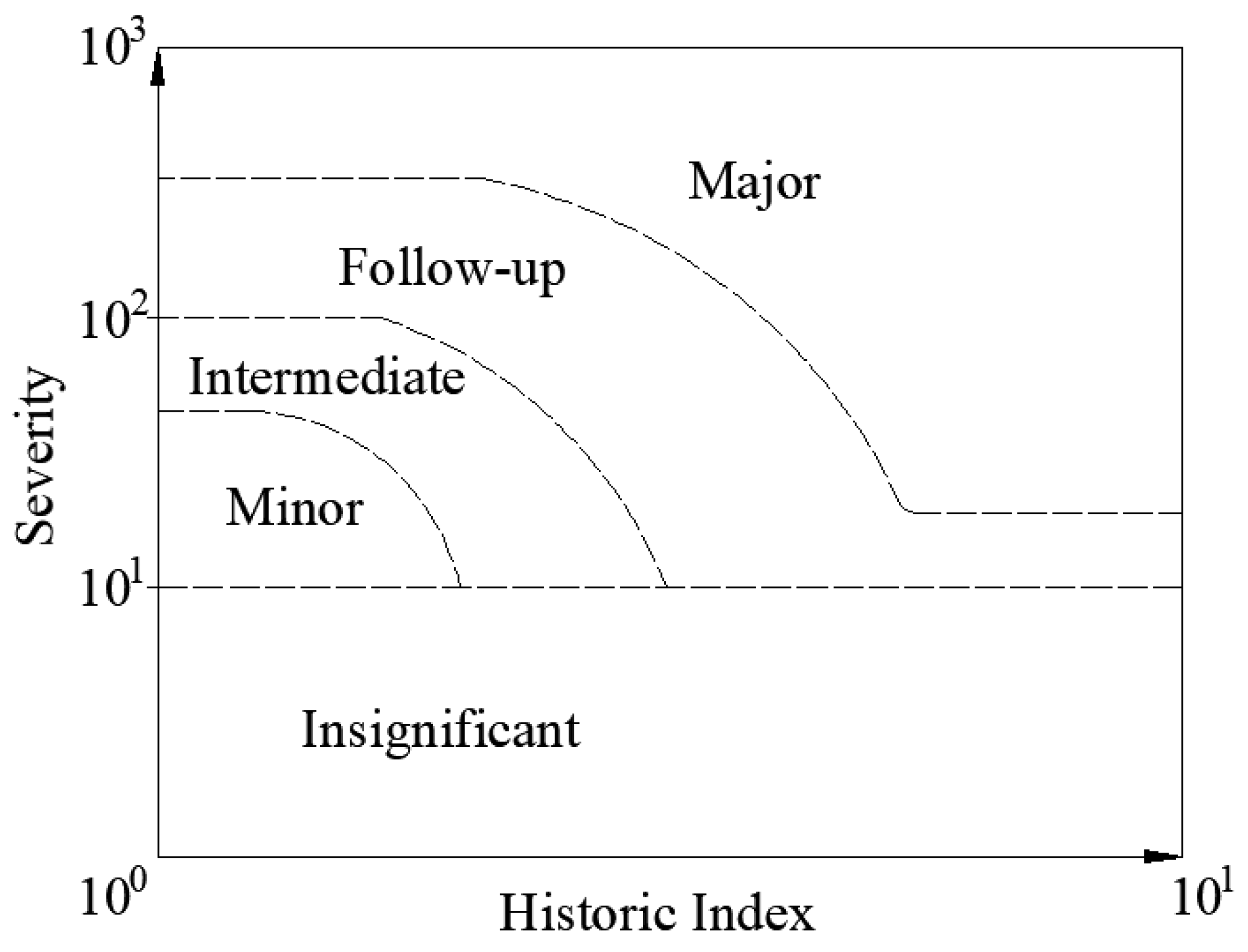
2. Parameter-Based AE Analysis

Parameter-based analysis, which assumes that AE signals can be characterized by a set of parameters, is a widely used approach for analyzing AE data [20]. Typical AE parameters, as defined in ASTM 1316, include amplitude, duration, rise time, energy, and signal strength. These AE parameters correlate with the magnitude of the AE source and changes in the material’s physical properties. In the AE monitoring of concrete materials and structures, these parameters have proven to be sensitive to detecting fracture growth and deterioration. For example, load ratio, calm ratio, and relaxation ratio have been developed to qualify and quantify damage in reinforced and prestressed beams under incremental cyclic load tests [21,22,23,24]. In addition, the b-value, defined as the slope of AE signal amplitude distribution, proved to be an effective index in relation to the accumulation of microcracks and of macrocrack formation [25,26,27]. Moreover, fracture mode differentiation was carried out based on the differences in average frequency and RA value [28,29,30,31]. Shiotoni et al. proposed an improved b-value analysis (Ib-value), drawing inspiration from seismic b-value analysis [32,33]. In this method, statistical values such as the mean (μ) and standard deviation (σ) of amplitude distribution are used to calculate the b-value. Meanwhile, the lower bound amplitude, the upper bound amplitude, and the range of amplitude are μ − α₂*σ, μ + α₁*σ, and (α₁ + α₂) *σ, respectively. Thus, the Ib-value can be calculated by the following equation:

$$Ib={\displaystyle \frac{{\log }_{10}(N(\mu -{\alpha }_2\sigma ))-{\log }_{10}(N(\mu +{\alpha }_1\sigma ))}{({\alpha }_1+{\alpha }_2)\sigma }}$$

(1)

where N represents the frequency of earthquakes within a specific range, while μ and σ denote the mean and standard deviation of AE amplitude, respectively. α₁ and α₂ are user-defined constants that define the lower and upper bounds of amplitude.

Intensity analysis is another parameter-based technique used to characterize damage levels and assess the overall integrity of test specimens [34,35]. The AE parameter signal strength, defined as the area under the signal envelope over its duration, is utilized in this method. Historic index (HI) and severity (S_r) are two indices derived from the signal strength data collected under the different loading conditions applied. The HI is a parameter determining the change in slope of the cumulative signal strength over time, which can be represented in the form of Equation (2), as follows:

$$HI={\displaystyle \frac{N}{N-K}}({\displaystyle \frac{{\displaystyle \sum _{i=K+1}^N{S}_{oi}}}{{\displaystyle \sum _{i=1}^N{S}_{oi}}}})$$

(2)

where N is the cumulative number of AE hits up to time t, S_oi is the signal strength of the ith hit, and K is an empirical factor which depends on the number of hits; if K < 50, K = 0; if 51 ≤ K < 200, K = N − 30; if 201 ≤ K < 500, K = 0.85 N; and if K ≥ 500, K = N − 75. Severity (S_r) is defined as the average signal strength of the J hits, usually 50 hits in concrete, with the largest numerical value of signal strength and is represented with Equation (3).

$$S_r={\displaystyle \frac{1}{J}}{\displaystyle \sum _{i=1}^J{S}_{oi}}$$

(3)

The level of damage can be determined by plotting the maximum HI and S_r values in the log-severity and log-historic index graph, as shown in Figure 3.

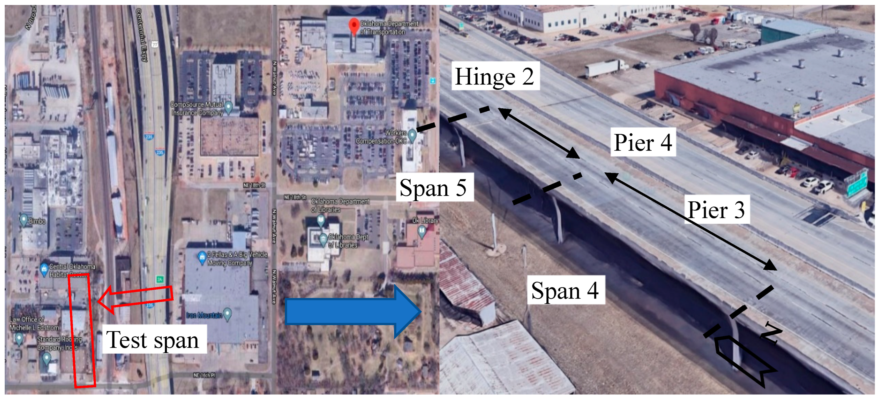
3. Experiment Program

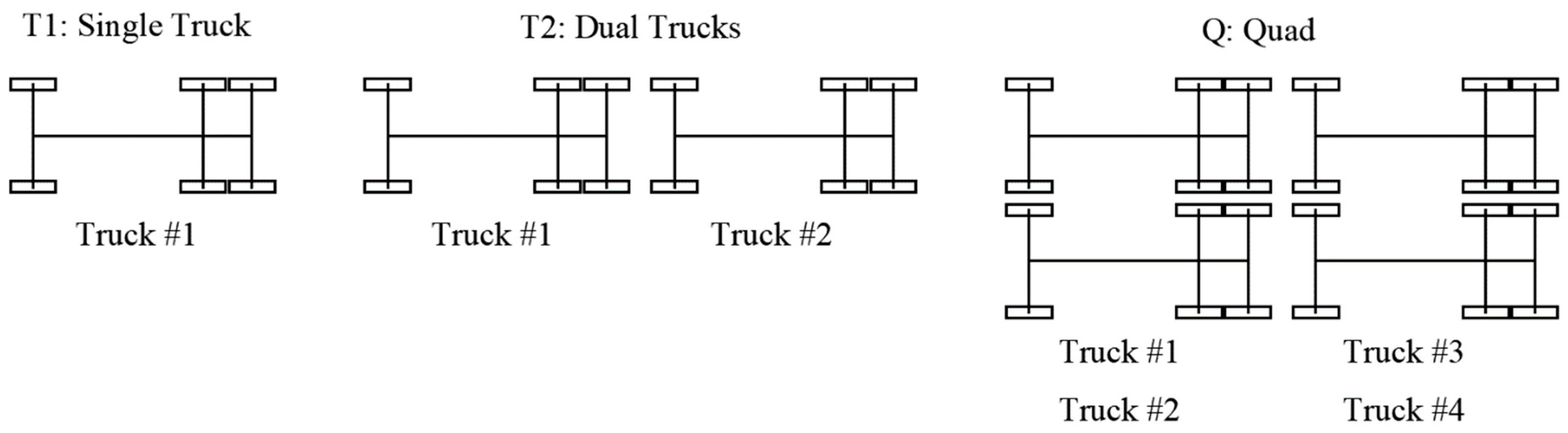
3.1. Load Test Protocol and Truck Information

In the bridge load test, the trucks of known weight were driving across the bridge along predetermined lines with the speed of 4.8 km/h (3 mph). The bridge monitoring under the moving vehicles was performed through strain measurement and AE monitoring at strategic sensor locations. Three predetermined load levels were used as the “live loads”. The individual layout for the different load levels is shown in Figure 4. The vehicles’ axle weight information is summarized in

Table 1. Axle and Gross Weight of Each Truck.

Truck Label	Front Axle Wt. (Kips)	Rear Axle Wt. (Kips)	Gross Wt. (Kips)
#1	13.12	39.64	52.76
#2	14.08	36.48	50.56
#3	11.46	33.66	45.12
#4	14.56	33.74	48.30

(Note: 1 kip = 453.6 kg).

. The lanes included west side shoulder (WL), centerline (CL), and east side shoulder (EL). Each lane experienced two identical passes for each separate “live load”. The load test protocol and nomenclature are shown in

Table 2. Bridge Load Test Protocol and Nomenclature.

Load Scenario	Total Weight (Kips)	Lane Tests
		West Lane (WL)	Center Lane (CL)	East Lane (EL)
Truck 1 Series (T1)	52.76	T1-WL-P1(P2)	T1-CL-P1(P2)	T1-EL-P1(P2)
Truck 2 Series (T2)	103.32	T2-WL-P1(P2)	T2-CL-P1(P2)	T2-EL-P1(P2)
Quads Series (Q)	196.74	Q-WL-P1(P2)	Q-CL-P1(P2)	Q-EL-P1(P2)

.

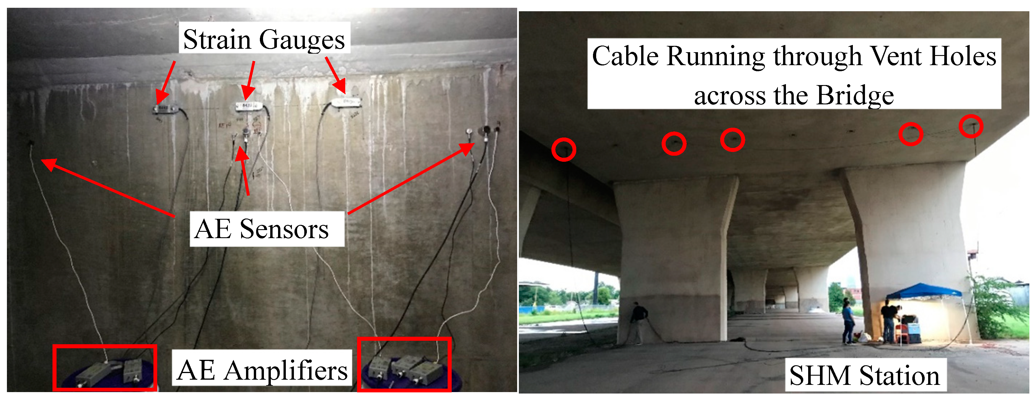
3.2. Strain Monitoring System

A BDI-STSII system from Bridge Diagnostics Inc. was used for strain monitoring in this project. It was composed of data acquisition hardware, ST350 strain gauges, and an STSII software with cables. The strain transducers were placed at the midspan and near the supports of the box girders—Web 1 (W1), Web 2 (W2), Web 3 (W3), Web 7 (W7), Web 8 (W8), and Web 9 (W9)—as shown in Figure 5. Three strain gauges were placed near the support area and one strain gauge was placed at the midspan on both sides of W2, W3, W7, and W8. For W1 and W9, the same setup of strain gauges was utilized but only on one side. The corresponding strain data at each test spot were recorded continuously at 50 Hz while the trucks moved across the bridge. An auto-clicker system was used to track the longitudinal position of the moving vehicle by sending a ‘click’ point to the STSII software when the front wheel of the truck had made one full rotation. Therefore, the structural strain response as a function of the moving truck’s position was obtained. During installation, the strain gauges were mounted on the surface of the evaluated members using epoxy glue after minimally grinding or sanding the cast concrete surface.

3.3. AE Monitoring System

A multichannel acoustic emission system Micro-II Express from Physical Acoustics Corporation (PAC) (West Windsor Township, NJ, USA) was used to perform the acoustic emission monitoring. Three types of AE sensors were used for monitoring the bridge section, namely R15I, R.45I with an integral preamplifier, and Wideband (WD). The R.45 and R15 sensors are narrow-band resonant-type AE sensors with peak frequencies of 20 kHz and 150 kHz, respectively, while the WD sensor is a differential wideband sensor with frequency response over a range of 100–900 kHz. To ensure the accuracy of the AE measurements, traffic was completely closed during the load test, eliminating potential noise interference from passing vehicles. The data acquisition threshold was set to 48 dB to minimize low-level background noise and external disturbances. The AE sensors were placed near the support area on both W2, the structurally sound control group, and W8, the experimental group or the area in need of repair. The detailed sensor layout and the types of different AE sensors are shown in Figure 6 and Figure 7, respectively. Figure 8 shows the photos regarding the sensors after installation and an overview of the test setup.

After grinding the surface of the test member, each sensor was bonded to the surface with a thin layer of hot glue. Then, the cable was restrained on the surface of the wall with tape to confine their movement during the cable running and transporting process. AEwin real-time AE data acquisition software was used to operate the AE system and visualize and recorded data during testing. Once the testing equipment was in place, a pencil-lead break test was carried out to verify the response of the sensors and AE system. Throughout the testing, the strain response and the activity from the acoustic emissions were recorded.

4. Results and Discussion

The reproducibility of the test results was graphically investigated by a comparison of the strain responses of two identical passes (P1 and P2) in each loading protocol. Figure 9 shows an example of a comparison in which the strain response is plotted with respect to the location of the moving load. The solid and dash lines correspond with the first and second load passes, respectively. The reversed x-axis load position remains consistent with the cardinal direction of the moving load shown on the schematic graph (Figure 5). The blue vertical dash lines indicate the position of different hinges or piers across the test spans, whereas the blue horizontal lines illustrate where the zero-strain is. It should be noted that the starting point PIER 5—22 ft before HINGE 2—used to record the strain response on the following graphs is not the same as the actual starting location of the test PIER 6—187 ft before HINGE 2. The truncation of the strain data while the truck(s) were moving from PIER 6 to PIER 5 is considered reasonable as the strain response during this period is almost zero.

Figure 9 presents the examples of the verification for two sensors located at the midspan and near-support area on W2. This set of figures illustrates that the sections’ strain responses at both test locations are overlapping for the two replicate passes, and that their maximum strain responses occur when the load trucks are at the same location, approximately 110 feet from HINGE 2. This demonstrates the consistency of the test results of two identical load passes. Moreover, strain response returns to zero after each load test which is evidence of linear behavior of the structure under given load levels.

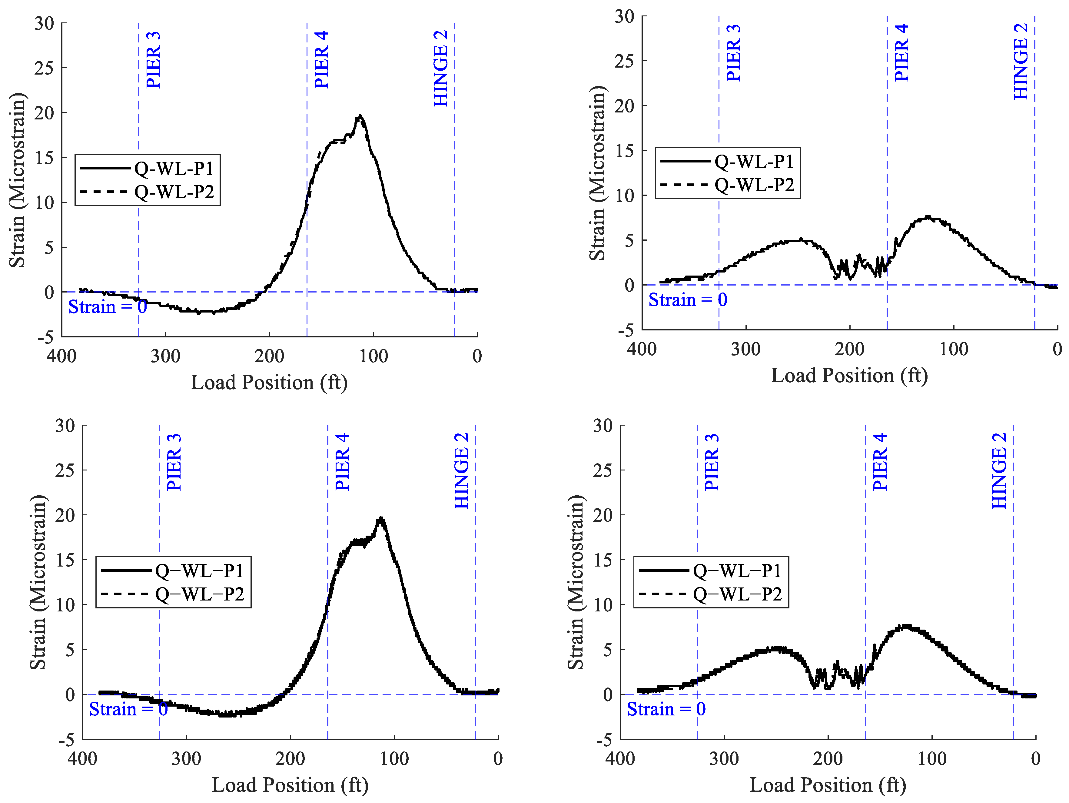
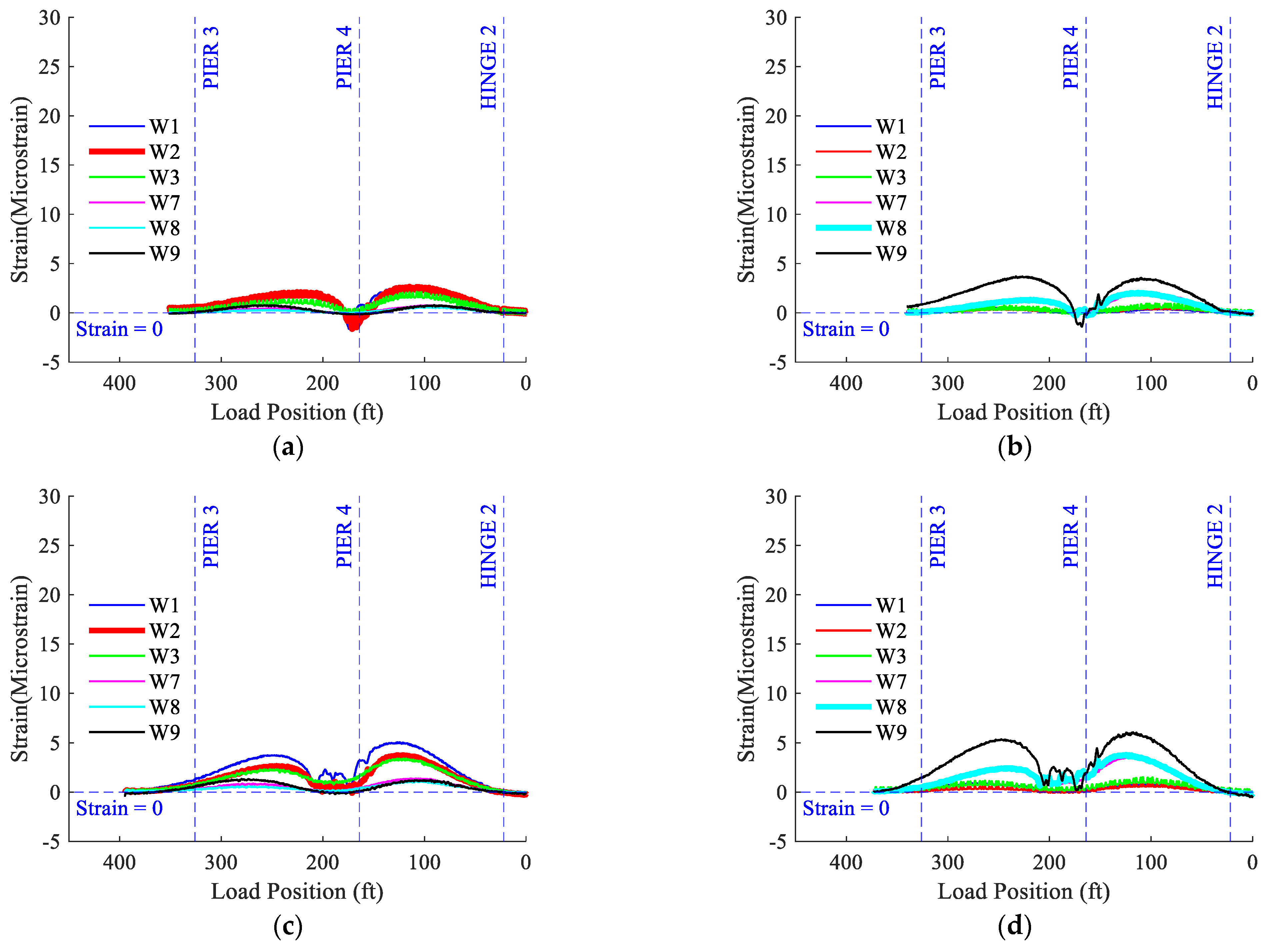
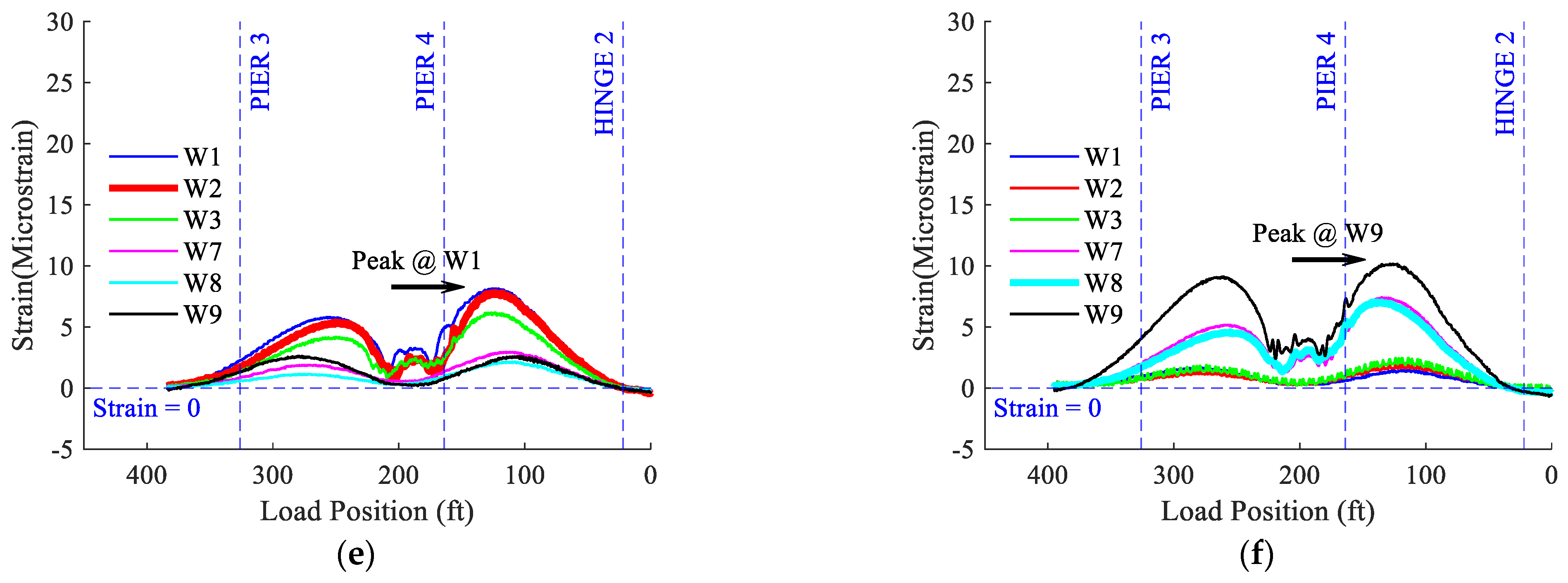
4.1. Comparison Analysis of Strain Responses Between Symmetric Locations

The strain measurements from symmetric locations were observed to draw comparisons between the behavior of the repaired side and that of the structurally sound side. Load passes QL1 and QL5 were symmetric load cases, and their corresponding strain results were examined as can be seen in the figures below. Figure 10 and Figure 11 plot the strain responses at the critical locations on W1, W2, W3, W7, W8, and W9 under all three tested load levels. It should be noted that the following strain responses are the average of all the effective gauges readings from the same location (midspan or near-support area). For comparison purposes, the strain results from the critical locations of W2 and W8 are highlighted by the thicker red and cyan lines, respectively. As shown in Figure 10, the maximum midspan strain response from Web 8 under T1-EL, T2-EL, and Q-EL are 11.56, 16.02, and 27.42, respectively, which are higher than the results of their corresponding mirror side under T1-WL, T2-WL, and Q-WL. This may result from a loss of the cross-section of prestressed strands in W8 due to corrosion. However, an overall similar strain response at symmetric spots of the structure is observed. For example, the magnitudes of the strain responses at both the midspan and the near support area on the other webs do not have significant differences with their corresponding mirror spots. In addition, the maximum near-support strain responses for W8 are even smaller than the ones for W2. Thus, all the above-mentioned observations may indicate a generally good condition of the bridge, as well as the effectiveness of the repair.

Moreover, similar performances between the repair side and the mirror structurally sound side can be found in the statistical analysis of their corresponding maximum responses.

Table 3. Comparison of maximum strain response under symmetric load.

Strain Response of W2				Strain Response of W8				F-Test (p-Value)	t-Test (p-Value)
L.P.	SG. Loc.	Avg.	CoV.	L.P.	SG. Loc.	Avg.	CoV.
T1-WL	Midspan	9.02	18.19%	T1-EL	Midspan	11.56	32.00%	0.532	0.469
	Support	2.73	17.75%		Support	1.86	40.55%	0.494	0.086
T2-WL	Midspan	12.93	16.92%	T2-EL	Midspan	16.02	30.40%	0.538	0.500
	Support	4.43	5.74%		Support	3.80	36.03%	0.020	0.369
Q-WL	Midspan	21.60	14.57%	Q-EL	Midspan	27.42	25.79%	0.533	0.399
	Support	8.00	8.39%		Support	7.15	35.78%	0.053	0.545

(Note: L.P. = Load Pass; SG. Loc. = Strain Gauge Location; Avg. = Average; CoV. = Coefficient of Variation).

presents the average maximum strain results from the gauges at the same spots on both sides, along with their coefficient of variation for each level. Again, the strain response at W2 serves as the control group for which the strain on the mirror side is obtained under symmetric load cases. The returned p-Value of the F-test and t-test conducted between the two sets is given to determine if significant differences exist in the standard deviations and means of the test results. A confidence level of 95% is used for that purpose. The high returned p-Value for each load case indicates no discernable changes in their means between the two datasets. Looking at the coefficient of variation (CoV) calculated for the critical spots on the sound sides, they vary between 5.7% and 18.19%. The overall high level of CoV obtained from the test may be due to the degraded material subjected to external loading. This is particularly distinguishable on the repair side, in which the CoV varies from 25.79% to 40.55%. The relatively high CoV observed in some measurements can be attributed to two primary factors. First, some sensors were placed on the repaired area where the new concrete may exhibit a different modulus of elasticity compared to the existing concrete. This variation in material properties could lead to increased variability in the data. Second, the relative strain measurements recorded were quite small, meaning that even minor fluctuations or noise in the data could significantly impact the CoV. While these factors contribute to variability, the overall trends in the data remain consistent, supporting the validity of the conclusions drawn from this study.

The linear relationship between the applied load level and the strain response is shown in Figure 12. The load and maximum strain in this set of graphs were normalized based on the gross vehicle weight and the maximum strain level obtained from the T1 series load cases. As shown in Figure 12, the R-squared value is very close to one in both cases, which indicates that both webs still undergo linear elastic deformation. This could be additional evidence that supports the overall good condition of the bridge. It should be noted that the maximum midspan strain for W2 and W8 during the T2 series are 1.440 and 1.383, respectively, times higher than the ones during T1 load cases. The increase in the truck weight from T1 to T2 is by a factor of 1.958, which is much higher than the strain increase. This is caused by the different truck layouts of the T1 and T2 series. The latter truck layout has a longer distributed load, which is double that of the T1 series. On the contrary, T2 and Q series have similar axle load distribution. As a result, the midspan strain of W2 and W8 during load case Q is 1.698 and 1.715 times higher than those during load case T2, which is close to the increase in gross vehicle weight of 1.904 times that of T2. However, it should be noted that the linear regression assumes that all three loading conditions are single-point loads, whereas the actual load conditions for the T2 and Q scenarios were spread more than the T1 scenario.

4.2. Comparison of AE Activity Between Symmetric Locations

In this section, the comparison of AE activity between the structurally sound side and the repaired side was carried out. It should be noted that only the R.45-type sensors received AE activity, while the other sensors were almost silent during the tests. It is reasonable that no visible cracks appeared during the testing, and that the lack of detected AE signals could be due to the high attenuation of the high-frequency sensors. Therefore, the AE activity from those sensor, along with strain responses, was plotted against the location of moving vehicles. A comparison of the results from both the test locations is demonstrated in Figure 13. The results from the sound side were on the right, whereas their counterparts from the repair area were on the left. As shown in this set of graphs, an increased trend of structural strain response was observed as the load level increased from T1 to Q. As for the AE activity, looking at the AE activity at the location with the peak strain response between HINGE 2 and PIER 4, there seems to be more AE hits on the repair side than on the structurally sound side for all the three load levels. This might be due to the interaction between the original concrete and the repair patch. Meanwhile, as the load increased, the AE activity seemed to remain unchanged to a similar extent. Most of the AE hits were below 60 dB, and the majority of them happened when the truck(s) were around PIER 4.

The b-value analysis was carried out in Matlab R2023b. A constant pattern was observed across all lanes, despite variations in the load levels (Figure 13). In the T1 series, the b-value remained relatively stable around two, with a slight increase towards the later stages, suggesting a steady material response. In the T2 series, a more noticeable drop in the b-value was observed initially, followed by a sharp increase, which may indicate microstructural changes. The Q series showed the highest variability, with frequent oscillations and spikes, particularly near the later points, which may indicate more localized stress redistributions compared to the steadier trends seen in T1 and T2 series. However, the b-value remained above one in all the loading scenarios, which typically indicates the absence of progressive damage as the load increases [36]. This is in line with the absence of cracks around the monitoring area. Similarly, the comparison of cumulative signal strength (CSS) and historic index (HI) was performed for the previous results. As seen from Figure 14, either on the repair side or the sound side, there was an increased trend of cumulative signal strength as the load level increased. Looking at the CSS in this set of graphs, a majority of the energy contribution was from the AE activity around PIER 4. This corresponds well with the AE pattern observed before. Meanwhile, the ‘knee’ in the cumulative signal strength curve (significant change in slope of the curve) matched with the sharp change in historic index curve for different load levels. Again, for each load level, there seemed to be slight increase in CSS in the repair area compared with the sound area. Intensity analysis was then carried out by plotting the maximum CSS and HI values from all three load levels on both the repair and structurally sound areas (Figure 15). The types of markers in the intensity chart indicate the different load levels, and the colors indicate the test locations. As shown in the graph, as the load level increased on both sides except load pass T2L5, the higher intensity points (with higher load levels) moved toward the top right corner, and vice versa. Overall, there were no significant differences between the intensity points from the sound and repair sides, although the latter seemed to move further toward the top right corner (Figure 16). This could be an indication of similar performance on both sides. Meanwhile, considering the lack of AE activity from the other types of sensors, it can be concluded that there was an overall good structural performance on both sides.

5. Conclusions

From the structural strain results, the reproducibility of the test results can be observed in most of the loading scenarios by comparisons of the strain responses between two identical paths. Moreover, an overall similar strain response at the symmetric spots can be obtained by a comparison of the magnitude of the strain response at several critical spots of the structural sound webs with their corresponding mirror spots. In addition, a linear relationship between the load level applied and the strain response is found. All the above-mentioned points indicate the generally good condition of the bridge and effectiveness of the repair.

For the AE activity of all the three load levels, there seems to be more AE hits and increasing AE CSS on the repair side than on the corresponding mirror side. This may have resulted from an interaction between the original concrete and the repair patch. Combined with the fact that no visible cracks are observed, and that AE activity is in a relatively low amplitude range on both sides, they might be frictional noise from the structural movement when the truck(s) were passing by. Again, there is no significant difference between the location of the intensity points and the sound and repair sides, although the latter seems to move further toward the top right corner. This could be additional evidence of the similar structural performance from both sides. Intensity analysis seems to be sensitive to the changes in structural performance, even though the change is extremely minor. A similar conclusion can be drawn from the b-value analysis, as it consistently remains above one across the different load testing scenarios. The relatively high b-value throughout the different load testing scenarios indicates no progressive damage and reflects structural soundness, which aligns with the absence of visible cracks in the monitored area.

While this study demonstrates the effectiveness of parameter-based AE analysis in assessing the repair performance of the bridge, it has certain limitations. Field monitoring using AEs requires further laboratory-scale testing to verify the potential sources of AE signals under controlled conditions. Additionally, future studies should incorporate signal-based AE analysis to explore the frequency content of AE signals using advanced signal processing techniques. This would provide a more detailed understanding of damage mechanisms and enhance the interpretation of AE data in field applications.

References

1. Trejo, D.; Hueste, M.; Gardoni, P.; Pillia, R.G.; Reinschmidt, K.; Im, S.B.; Kararia, S.; Hurlebau, S.; Gamble, M.; Ngo, T.T. Effect of Voids Grouted Post-Tensioned Concrete Bridge Construciton—Volume 1—Electrochemical Testing And Reliability Assessment; Texas Department of Transportation: Austin, TX, USA, 2009.
2. Menga, A.; Kanstad, T.; Cantero, D.; Bathen, L.; Hornbostel, K.; Klausen, A. Corrosion-induced damages and failures of posttensioned bridges: A literature review. Struct. Concr. 2022, 24, 84–99. [Google Scholar] [CrossRef]
3. Sun, Z.; Wang, X.; Han, T.; Huang, H.; Ding, J.; Wang, L.; Wu, Z. Pipeline deformation monitoring based on long-gauge fiber-optic sensing systems: Methods, experiments, and engineering applications. Measurement 2025, 248, 116911. [Google Scholar] [CrossRef]
4. Nasir, V.; Ayanleye, S.; Kazemirad, S.; Sassani, F.; Adamopoulos, S. Acoustic emission monitoring of wood materials and timber structures: A critical review. Constr. Build. Materials 2022, 350, 128877. [Google Scholar] [CrossRef]
5. Ono, K. Review on Structural Health Evaluation with Acoustic Emission. Appl. Sci. 2018, 8, 958. [Google Scholar] [CrossRef]
6. Sagar, R.V.; Prasad, B.K.R. A review of recent developments in parametric based acoustic emission techniques applied to concrete structures. Nondestruct. Test. Evaluation 2012, 27, 47–68. [Google Scholar] [CrossRef]
7. Ciaburro, G.; Iannace, G. Machine-Learning-Based Methods for Acoustic Emission Testing: A Review. Appl. Sci. 2022, 12, 10476. [Google Scholar] [CrossRef]
8. Carpinteri, A.; Lacidogna, G.; Accornero, F.; Mpalaskas, A.C.; Matikas, T.E.; Aggelis, D.G. Influence of damage in the acoustic emission parameters. Cem. Concr. Compos. 2013, 44, 9–16. [Google Scholar] [CrossRef]
9. Elfergani, H.A.; Pullin, R.; Holford, K.M. Damage assessment of corrosion in prestressed concrete by acoustic emission. Constr. Build. Mater. 2013, 40, 925–933. [Google Scholar] [CrossRef]
10. Shahid, K.A.; Bunnori, N.M.; Megat Johari, M.A.; Hassan, M.H.; Sani, A. Assessment of corroded reinforced concrete beams: Cyclic load test and acoustic emission techniques. Constr. Build. Mater. 2020, 233, 117291. [Google Scholar] [CrossRef]
11. Appalla, A.; ElBatanouny, M.K.; Velez, W.; Ziehl, P. Assessing Corrosion Damage in Posttensioned Concrete Structures Using Acoustic Emission. J. Mater. Civ. Eng. 2016, 28, 04015128. [Google Scholar] [CrossRef]
12. Farhidzadeh, A.; Dehghan-Niri, E.; Salamone, S.; Luna, B.; Whittaker, A. Monitoring Crack Propagation in Reinforced Concrete Shear Walls by Acoustic Emission. J. Struct. Eng. 2013, 139, 04013010. [Google Scholar] [CrossRef]
13. Zeng, H.; Hartell, J.A. Identification of Acoustic Emission Signatures and Their Capability to Assess the Damage of Reinforced Concrete Beam under Incremental Cyclic Loading. J. Mater. Civ. Eng. 2022, 34, 04022085. [Google Scholar] [CrossRef]
14. Van Steen, C.; Nasser, H.; Verstrynge, E.; Wevers, M. Acoustic emission source characterisation of chloride-induced corrosion damage in reinforced concrete. Struct. Health Monit. 2021, 21, 1266–1286. [Google Scholar] [CrossRef]
15. Elbatanouny, E.; Ai, L.; Henderson, A.; Ziehl, P. An automated load determination approach for concrete girder bridges through acoustic emission. Adv. Struct. Eng. 2024, 28, 159–178. [Google Scholar] [CrossRef]
16. Laxman, K.C.; Ross, A.; Ai, L.; Henderson, A.; Elbatanouny, E.; Bayat, M.; Ziehl, P. Determination of vehicle loads on bridges by acoustic emission and an improved ensemble artificial neural network. Constr. Build. Mater. 2023, 364, 129844. [Google Scholar] [CrossRef]
17. Anay, R.; Lane, A.; Jauregui, D.; Weldon, B.; Soltangharaei, V.; Ziehl, P. On-Site Acoustic-Emission Monitoring for a Prestressed Concrete BT-54 AASHTO Girder Bridge. J. Perform. Constr. Facil. 2020, 34, 04020034. [Google Scholar] [CrossRef]
18. Pirskawetz, S.M.; Schmidt, S. Detection of wire breaks in prestressed concrete bridges by Acoustic Emission analysis. Dev. Built Environ. 2023, 14, 100151. [Google Scholar] [CrossRef]
19. Käding, M.; Schacht, G.; Marx, S. Acoustic Emission analysis of a comprehensive database of wire breaks in prestressed concrete girders. Eng. Struct. 2022, 270, 114846. [Google Scholar] [CrossRef]
20. Godin, N.; Reynaud, P.; Fantozzi, G. Acoustic Emission and Durability of Composite Materials; ISTE Ltd.: London, UK; John Wiley & Sons, Inc.: Amsterdam, The Netherlands, 2018; Volume 3. [Google Scholar]
21. Ohtsu, M.; Uchita, M.; Okamoto, T.; Yuyama, S. Damage assessment of reinforced concrete beams qualified by acoustic emission. ACI Struct. J. 2002, 99, 411–417. [Google Scholar]
22. Ridge, A.R.; Ziehl, P.H. Evaluation of Strengthened Reinforced Concrete Beams: Cyclic Load Test and Acoustic Emission Methods. ACI Struct. J. 2006, 103, 832–841. [Google Scholar]
23. Colombo, S.; Forde, M.C.; Main, I.G.; Shigeishi, M. Predicting the ultimate bending capacity of concrete beams from the “relaxation ratio” analysis of AE signals. Constr. Build. Mater. 2005, 19, 746–754. [Google Scholar] [CrossRef]
24. Sagar, V.; Prasad, R. Damage limit states of reinforced concrete beams subjected to incremental cyclic loading using relaxation ratio analysis of AE parameters. Constr. Build. Mater. 2012, 35, 139–148. [Google Scholar] [CrossRef]
25. Colombo, S.; Main, I.G.; Forde, M.C. Assessing Damage of Reinforced Concrete Beam Using “b-value’’ Analysis of Acoustic Emission Signals. J. Mater. Civ. Eng. 2003, 15, 280–286. [Google Scholar] [CrossRef]
26. Farhidzadeh, A.; Salamone, S.; Luna, B.; Whittaker, A. Acoustic emission monitoring of a reinforced concrete shear wall by b-value–based outlier analysis. Struct. Health Monit. Int. J. 2012, 12, 3–13. [Google Scholar] [CrossRef]
27. Kurz, J.H.; Finck, F.; Grosse, C.U.; Reinhardt, H.W. Stress drop and stress redistribution in concrete quantified over time by the b-value analysis. Struct. Health Monit. 2006, 5, 69–81. [Google Scholar] [CrossRef]
28. Ohno, K.; Ohtsu, M. Crack classification in concrete based on acoustic emission. Constr. Build. Mater. 2010, 24, 2339–2346. [Google Scholar] [CrossRef]
29. Aggelis, D.G.; Mpalaskas, A.C.; Matikas, T.E. Investigation of different fracture modes in cement-based materials by acoustic emission. Cem. Concr. Res. 2013, 48, 1–8. [Google Scholar] [CrossRef]
30. Zaki, A.; Chai, H.K.; Behnia, A.; Aggelis, D.G.; Tan, J.Y.; Ibrahim, Z. Monitoring fracture of steel corroded reinforced concrete members under flexure by acoustic emission technique. Constr. Build. Mater. 2017, 136, 609–618. [Google Scholar] [CrossRef]
31. Aggelis, D.G.; El Kadi, M.; Tysmans, T.; Blom, J. Effect of propagation distance on acoustic emission fracture mode classification in textile reinforced cement. Constr. Build. Mater. 2017, 152, 872–879. [Google Scholar] [CrossRef]
32. Shiotani, T.; Fujii, K.; Aoki, T.; Amou, K. Evaluation of progressive failure using AE sources and improved b-value on slope model tests. In Proceedings of the Progress in Acoustic Emission VII, Sapporo, Japan, 17–20 October 1994; pp. 529–534. [Google Scholar]
33. Shiotani, T.; Yuyama, S.; Li, Z.W.; Ohtsu, M. Application of the AE improved b-value to qualitative evaluation of fracture process in concrete materials. J. Acoust. Emiss. 2001, 19, 118–132. [Google Scholar]
34. Di Benedetti, M.; Nanni, A. Acoustic Emission Intensity Analysis for In Situ Evaluation of Reinforced Concrete Slabs. J. Mater. Civ. Eng. 2014, 26, 6–13. [Google Scholar] [CrossRef]
35. Fowler, T.J.; Blessing, J.A.; Conlisk, P.J.; Swansong, T.L. The MONPAC system. J. Acoust. Emiss. 1989, 8, 1–8. [Google Scholar]
36. Zeng, H.; Hartell, J.A.; Soliman, M. Damage evaluation of prestressed beams under cyclic loading based on acoustic emission monitoring. Constr. Build. Mater. 2020, 255, 119235. [Google Scholar] [CrossRef]
Figure 1. Location of test spans.
Infrastructures 10 00056 g001
Figure 2. Distress features in PT ducts: grouting voids (left) and corrosion products (right) (Note: Published with the permission from ODOT bridge division).
Infrastructures 10 00056 g002
Figure 3. Intensity chart showing different degrees of damage of material (adapted from [35]).
Infrastructures 10 00056 g003
Figure 4. Truck layout for three load levels.
Infrastructures 10 00056 g004
Figure 5. Schematic graph of the bridge spans and strain gauge layout.
Infrastructures 10 00056 g005
Figure 6. Schematic of AE sensor layout on W2 (left) and W8 (right).
Infrastructures 10 00056 g006
Figure 7. Types of AE sensors.
Infrastructures 10 00056 g007
Figure 8. AE sensor and strain gauge installation inside bridge cell (left) and setup of SHM system onsite (right).
Infrastructures 10 00056 g008
Figure 9. Comparison of strain response between two identical passes at W2 midspan (left) and W2 near-support (right).
Infrastructures 10 00056 g009
Figure 10. Midspan Strain under Symmetrically Applied Load: (a) Load pass T1-WL; (b) Load pass T1-EL; (c) Load pass T2-WL; (d) Load pass T2-EL (e) Load pass Q-WL; (f) Load pass Q-EL.
Infrastructures 10 00056 g010
Figure 11. Near-Support Strain under Symmetrically Applied Load: (a) Load pass T1-WL; (b) Load pass T1-EL; (c) Load pass T2-WL; (d) Load pass T2-EL (e) Load pass Q-WL; (f) Load pass Q-EL.
Infrastructures 10 00056 g011aInfrastructures 10 00056 g011b
Figure 12. Linear relationship between normalized load and maximum strain under three different load levels: (a) Midspan strain on W2 during T1-WL, T2-WL and Q-WL; (b) Midspan strain on W8 during T1-EL, T2-EL and Q-EL.
Infrastructures 10 00056 g012
Figure 13. Comparison of strain and amplitude of AE Activity between Web 2 and Web 8 under different loading levels. (a) T1WLP1, (b) T1ELP1, (c) T2WLP1, (d) T2ELP1, (e) QWLP1, (f) QELP1.
Infrastructures 10 00056 g013
Figure 14. b-value analysis between Web 2 and Web 8 under different loading levels. (a) T1WLP1, (b) T1ELP1, (c) T2WLP1, (d) T2ELP1, (e) QWLP1, (f) QELP1.
Infrastructures 10 00056 g014
Figure 15. Comparison of HI and CSS between Web 2 and Web 8 under different loading levels. (a) T1WLP1, (b) T1ELP1, (c) T2WLP1, (d) T2ELP1, (e) QWLP1, (f) QELP1.
Infrastructures 10 00056 g015
Figure 16. AE intensity analysis for the repair and sound area.
Infrastructures 10 00056 g016