Abstract
Reinforced Concrete (RC) barriers are used for different purposes in the highway inventory. An important purpose is the use of concrete barriers to act as railing that protects bridge piers against vehicular collision force (VCF). Therefore, these barriers are designed to absorb the collision energy and/or redirect the vehicle away from the parts being protected. Accurate estimation of the capacity of RC barriers during crash events is an important consideration in their design and placement. The American Association of State Highway and Transportation Officials (AASHTO) considers yield line analysis (YLA) with the V-shape failure pattern to predict the barrier capacity. AASHTO’s analysis method involves some assumptions that are intended to simplify the analysis process. Some of these assumptions have been shown to underestimate the actual barrier capacity and might disqualify many existing RC barriers from acting as intervening structures due to structural inadequacy. Many researchers have proposed alternative failure patterns and methodologies in an attempt to better predict the capacity of RC barriers. This research shows that AASHTO’s YLA, with the current V-shape failure pattern, can be improved and still predict the barrier capacity when some of the simplifying assumptions are eliminated. Also, the research presents an alternative innovative truss analogy model to predict the capacity of RC barriers. The results of the improved YLA and the proposed truss model are validated by finite element analysis (FEA) using Abaqus. The results of this research will help structural engineers in the highway industry to initially design new barriers for the intended capacity as well as estimate the capacity of existing ones.
1. Introduction
Reinforced concrete (RC) barriers are widely used in transportation infrastructures for different purposes. For instance, median barriers are used to separate opposing lanes of traffic, and railing barriers are used to prevent vehicles accessing roadway shoulders and protect sign structures and pedestrians. In addition, it is very common to find RC barriers used as intervening structures protecting bridge piers against vehicular collision force (VCF). Therefore, estimating the capacity of these barriers when subjected to VCF is an important consideration in their design and placement.
The framework that leads to a successful placement of these barriers includes three main factors: knowing the required performance level, accurately analyzing and designing the barrier to meet the demands of the required performance level and testing the barrier to ensure satisfying the acceptance criteria. Among the previous three factors, the second one seems to be the most challenging. The reason is simply because one can set objectives (performance levels), and measures to decide whether the objectives are met (acceptance criteria), yet the methodology is what leads to achieving the objectives.
The first document that considered specifying the performance levels and the acceptance criteria was the NCHRP-Report 350 published in 1993 [1]. The performance levels, referred to as “Test Levels (TLs)”, in the NCHRP-Report 350, differ according to the impact conditions. A specific impact condition is a function of the vehicle designation (passenger car, single unit truck, tractor-semitrailer, etc.), the impact speed, and the impact angle. Higher TLs involve more severe impact conditions such as heavy vehicles travelling at high velocity. The same document included the acceptance criteria which were in three categories: structural adequacy, occupant risk, and post-impact vehicular trajectory. The criteria imply that, for a test article (barrier) to be acceptable for a certain TL, it has to be structurally adequate to dissipate the energy of the impacting vehicle specified for that TL without excessive damage to the barrier or penetration. Also, minimizing the risk of occupant injury and any potential subsequent multivehicle accident (bringing the impacting vehicle to a controlled stop).
The NCHRP-Report 350 recommended procedures that were implemented by the Federal Highway Administration (FHWA) in 1998. About a decade later, the American Association for State Highway and Transportation Officials (AASHTO) published a Manual for Assessing Safety Hardware (MASH) in 2009. This manual upgraded the impact conditions presented in NCHRP-Report 350 for some TLs to reflect more damaging crash events and produce more robust barriers for certain applications. The latest MASH was published in 2016 [2], and is currently adopted by AASHTO’s LRFD Bridge Design Specifications (Section 13) to define the TLs that will decide the design forces for traffic railings [3]. The different TLs as per MASH are shown in Table 1.

Table 1.
MASH test levels.
After knowing the performance level and the acceptance criteria, the challenging task becomes designing the barrier to meet the performance level and pass the acceptance criteria. This is typically achieved through designing barriers to resist certain levels of loading and satisfy geometry proportioning. For example, Table A13.2.1 in AASHTO LRFD Bridge Design Specifications [3] shows the design forces and designation for traffic railing required for different TLs.
The most common analysis method used to assess the structural capacity of barriers is the Yield Line Analysis (YLA). It was first introduced by Hirsch et al. [4], and is currently adopted by AASHTO’s LRFD Bridge Design Specifications (Section 13). This method is based on equating the work done by the external applied forces and the internal energy developed through the formation of yield lines due to triangular (V-shape) failure pattern. However, the current AASHTO’s procedure of YLA includes some assumptions to simplify the analysis process.
Many researchers criticized the simplified AASHTO’s procedure of YLA in terms of the capacity estimation and the failure pattern. Jeon et al. conducted a full-scale test varying the loading patterns to simulate vehicle crash. Contrary to the findings of this study, the results revealed a lower load capacity than that predicted by AASHTO’s equations and a different failure pattern that looks more like W-shape [5]. This failure pattern is agreed on by Cao et al. through dynamic explicit numerical simulations as well as quasi-static pushover analysis [6]. Loken et al. referred to the suggested W-shape as the modified YLA and made a comparison between the traditional V-shape and the modified W-shape failure patterns in terms of punching shear capacities. The study suggested that a significant increase in the punching shear capacity exists in the modified YLA [7]. While punching shear is a possible failure mechanism that was reported in many studies [8,9,10], it is less likely for this failure mode to control when enough transverse reinforcement is available.
The existing literature seems to agree that the current AASHTO’s procedure of YLA needs to be subject to further research. In this context, a distinction needs to be made between using AASHTO’s YLA as an initial qualifier for proposed barrier designs and judging the strength of existing barriers for decisions related to their structural capacity and crashworthiness. The former is a conservative analysis that will produce barriers designed with higher capacity than needed. On the other hand, the latter is a conservative analysis that will underestimate the actual strength of RC barriers. Such underestimation might lead to decisions like upgrading barriers by either replacement or retrofitting. While both cases seem to have negative economic effects, underestimating the capacity of existing RC barriers has more significance. This is due to the increase in load demands for some TLs that have been upgraded in MASH 2016, which disqualified many of the existing barriers from being structurally adequate for their intended purpose.
An example of the first case is the proposed design and development of a TL-5 RC barrier by Rosenbaugh et al. where AASHTO’s procedure of YLA was used to verify the initial loading capacity and geometric requirements as per Table A13.2.1 [3]. Then the barrier underwent cycles of design cost optimization before it was subjected to an actual TL-5 crash event to pass the acceptance criteria [11].
On the other hand, Bullrad et al. reported an experimental study of different crash tests according to the upgraded MASH requirements to evaluate the performance of commonly existing barriers. It was reported that 45% of the tested barriers failed to meet the acceptance criteria due to vehicle rolling over. No significant damage such as major structural cracks or penetration of the barrier was observed [12]. Although this reason is sufficient to disqualify the barrier, this failure is related to geometrical deficiency (insufficient height).
For this purpose, a numerical dynamic analysis study conducted by Salahat et al. estimated the VCF transferred to bridge piers in the presence of a disqualified RC Jersey barrier as a protective structure to bridge piers (referred to as sub-standard barrier in their study). The results showed that the sub-standard barrier was able to reduce the equivalent static load demand by at least 25%. Interestingly, it was reported that the remaining load transferred to the pier was due to the contact between the cargo area and the pier; no structural damage or penetration of the barrier was observed [13,14]. To further support this argument, Salahat et al. conducted a study to assess the performance of a sub-standard barrier subjected to high TLs (TL-4 and TL-5) the same conclusion was driven, stating that no significant structural damage or penetration was reported, and the structural inadequacy relates to geometrical differences [15].
Therefore, it is crucial to have guidance on accurate analysis methods and procedures that can estimate the structural capacity of RC barriers. This will help distinguish the geometrical deficiencies from the structural inadequacy as it relates to the acceptance criteria. For this purpose, this research presents an improved YLA according to the current and common V-shape failure pattern. Many of the simplifying assumptions will be eliminated and a clear analytical solution will be presented.
Also, an original and innovative alternative method is presented to predict the lateral capacity of RC barriers using a truss analogy model. The developed model provides guidelines on how to simulate the RC barrier as an equivalent space truss, thus avoid analyzing the complex interaction between steel and concrete materials in the barrier. A similar effort was made recently by Kim et al. who introduced a node-independent model to evaluate the capacity of RC barriers under VCF, the model tracks the yielding of nodes in the steel beam elements that derive their stresses from the master concrete solid elements. Their investigation suggested that a variation in the results exists when the bridge deck was modeled [16]. The approach presented in this paper tracks the formation of the V-shaped yield lines through incremental analysis.
Finally, a case study of an RC barrier will be analyzed using three different techniques: the improved YLA, the equivalent truss method, and numerical finite element analysis (FEA) using Abaqus to validate the forementioned methods. The findings confirmed the accuracy of the proposed solutions.
2. AASHTO’s Procedure of YLA
The simplified YLA procedure by AASHTO implements several assumptions, some of which are reasonable to assume but others may yield significant underestimation of the RC barrier capacity. These assumptions are summarized as:
- The deck has sufficient resistance to the applied transverse forces thus the yield line failure pattern will remain within the parapet.
- The presence of sufficient longitudinal length of the parapet to produce the assumed V-shape yield line failure pattern.
- The flexural capacity of the RC barrier is only from the concrete contribution; the contribution of the stirrups and/or ties is to prevent shear and diagonal tension.
- The wall resistance is the average of its value along the height when the width of the barrier varies along the height.
- The negative and positive wall resisting moments are equal
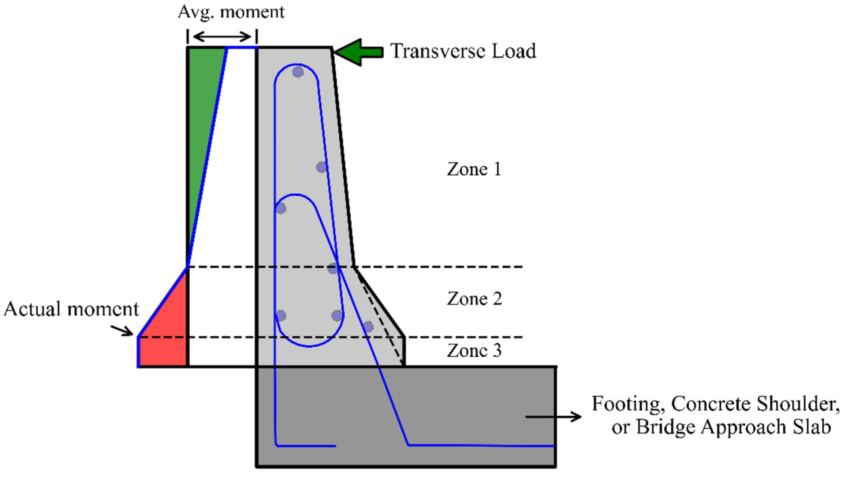
In the three assumptions, the deck slab is usually heavily reinforced to provide sufficient anchorage to the parapet dowels; and barriers usually run for distances long enough to ensure the development of the yield lines according to the suggested V-shape failure pattern. Also, in the third assumption, it is reasonable to consider longitudinal and vertical reinforcement to only contribute to the flexural capacity. However, the last two assumptions seem to be causing underestimation and will be subject to improvement in this paper. In the fourth assumption, the cantilever action produces a moment around an axis parallel to the longitudinal axis of the bridge. The moment demand has a linear function that is minimum at the top of the barrier and peaks at the support. Therefore, averaging the sectional capacity along the height reduces the flexural capacity at locations of high demand and increases the capacity where it is not needed as shown in Figure 1. The three zones in Figure 1 indicate that the flexural capacity function has geometrical (width) discontinuity along the height of the barrier. The same applies when calculating the capacity function around an axis that is vertical to the longitudinal axis of the bridge.
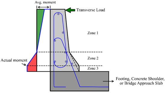
Figure 1.
Variation of the actual vs. the assumed moment capacity.
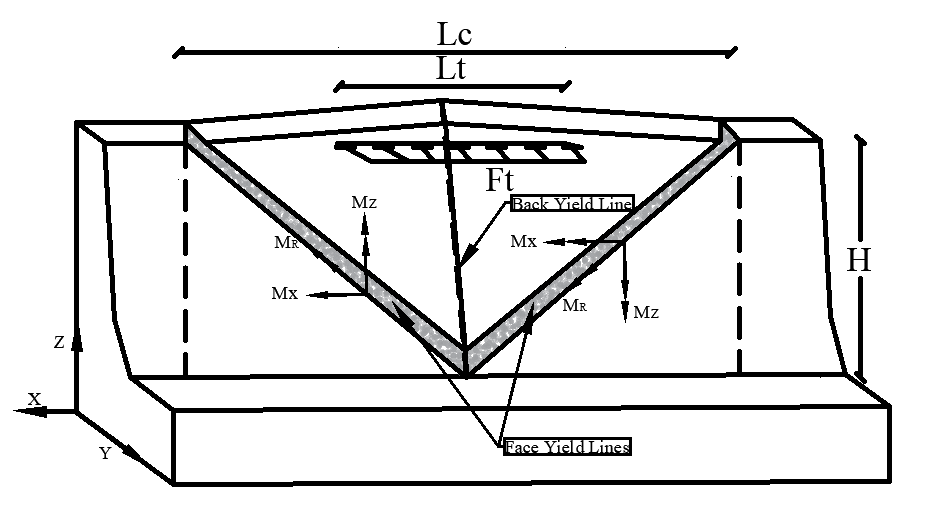
For the final assumption, equating the positive and negative resisting moment will not make a big difference because of assumption four. This is true when the barrier has uniform width and equal longitudinal reinforcement on both faces. Minor variation between the positive and negative sectional capacities happens around the longitudinal axis (x-axis in Figure 2). This is because each side will have the same number of stirrups legs. However, the major variation is in the sectional capacity around the vertical axis (z-axis in Figure 2), which is lower at the back side of the barrier (less longitudinal rebar in this barrier type). This lower capacity will conservatively be used for both positive and negative moments as per assumption five above. According to the proposed V-shape failure pattern, this lower resistance coming from the positive moment will represent the two front yield lines in terms of the resisting components around the vertical axis, Mz in Figure 2. Therefore, one can see how the error imposed by these assumptions accumulates to result in an underestimation of the barrier’s transverse capacity. Based on the previous assumptions, the current equations as per AASHTO LRFD Bridge Design Specifications (Section 13) [3] are given in Equations (1) and (2).
where:
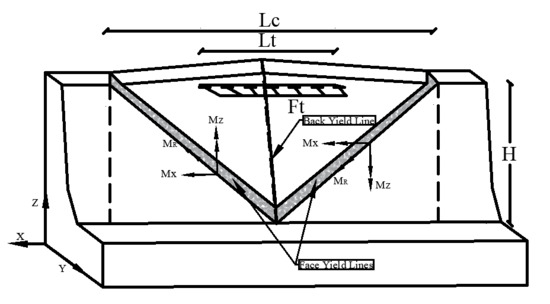
Figure 2.
Difference in negative and positive moments capacities at face yield lines and back yield line.
Rw = total transverse resistance of the railing (kips)
Lc = critical length of yield line failure pattern (ft)
Lt = longitudinal length of distribution of impact force Ft (ft), specified in (Table A13.2-1) [3]
Mb = additional flexural resistance of beam in addition to Mz, if any, at top of wall (kip-ft)
Mx = flexural resistance of cantilevered walls about an axis parallel to the longitudinal axis of the bridge (kip-ft/ft), (referred to as Mc in AASHTO’s specifications).
Mz = flexural resistance of the wall about its vertical axis (kip-ft), (referred to as Mw in AASHTO’s specifications).
H = height of wall (ft)
The total transverse resistance Rw should be equal or greater than Ft, the resultant transverse force specified in (Table A13.2-1) [3] and assumed to be acting at top of a concrete wall.
3. Improved YLA of RC Barriers
The procedure explained in this section is targeted to cover the generalized case of RC barriers where the barrier width is not uniform along its height and the positive and negative flexural capacities are not equal due to differences in reinforcement distribution at the back and front face of the barrier. This procedure covers other simple barriers configurations such as when the barrier has uniform width along its height, or the reinforcement is similar on both faces.
3.1. Sectional Capacity
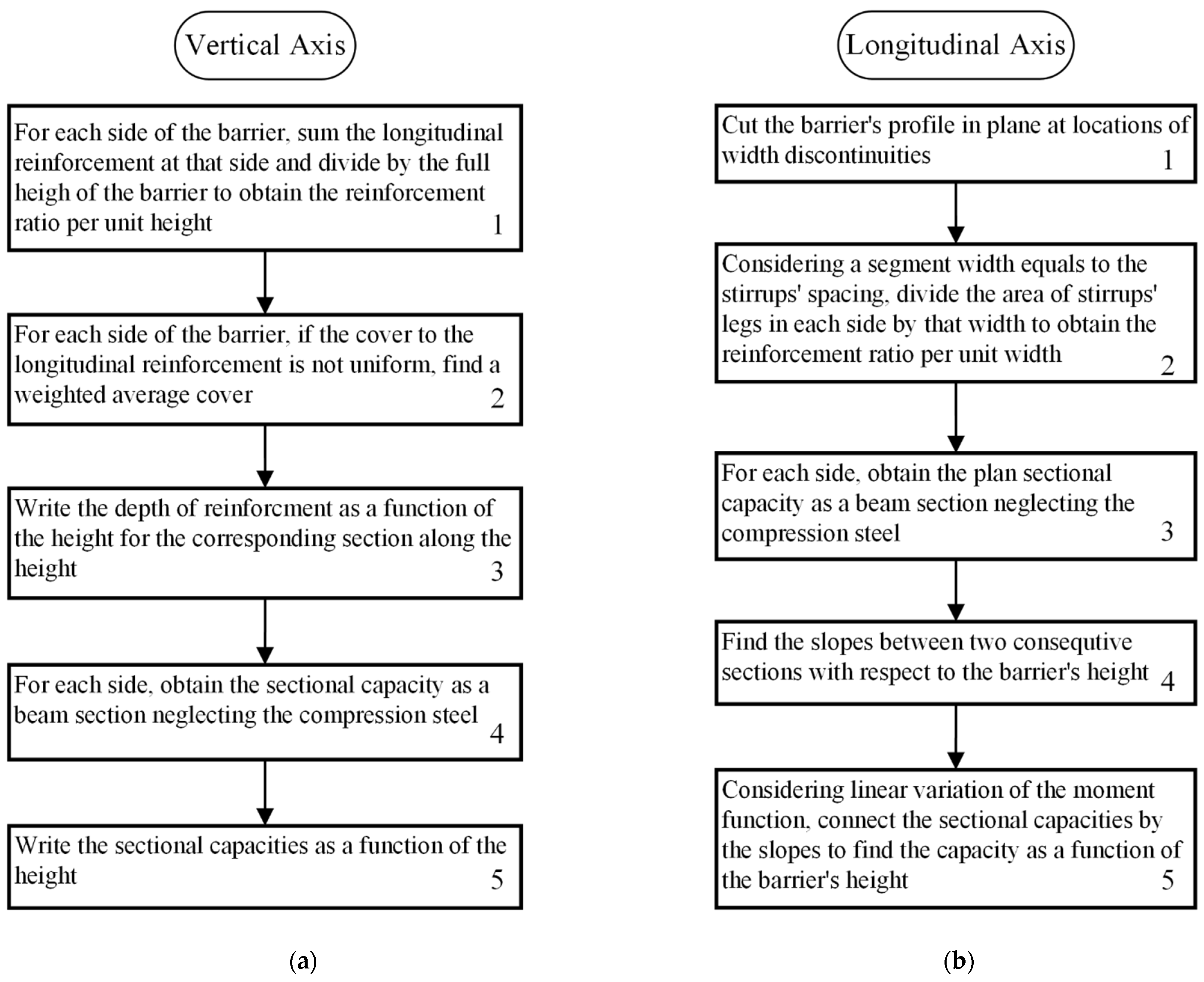
The flexural capacity around certain axis is found after dividing the barrier into different sections at the locations of geometrical discontinuities. For simplicity, the moment function of zone 2 is merged with that of zone 3 by following sloped dotted line in Figure 1. The procedure for obtaining the sectional flexural capacity around the vertical and longitudinal axes is shown in Figure 3a and Figure 3b respectively. The procedures shown in Figure 3 will be applied in detail in the case study section.

Figure 3.
Procedure to obtain sectional capacity around (a) vertical axis (b) longitudinal axis.
3.2. Formation of Yield Lines
The following are the assumptions that were made to develop the yield line analysis.
- Deformations and strains through the thickness are neglected in accordance with typical plate and shell assumptions. Therefore, the rotation of the vertical surface (back face of barrier) directly corelates to the rotation of an inclined surface (front face of barrier).
- For barriers that have sloped sides, the value of the deformation angle measured with respect to an assumed vertical plane and the deformation angle of the actual sloped side is almost the same. Therefore, the angle used in the derivations are referenced with respect to the vertical plane.
- The capacity of barrier is controlled by its flexural resistance. Shear failures are assumed to be avoided through sufficient distribution of transverse reinforcement.
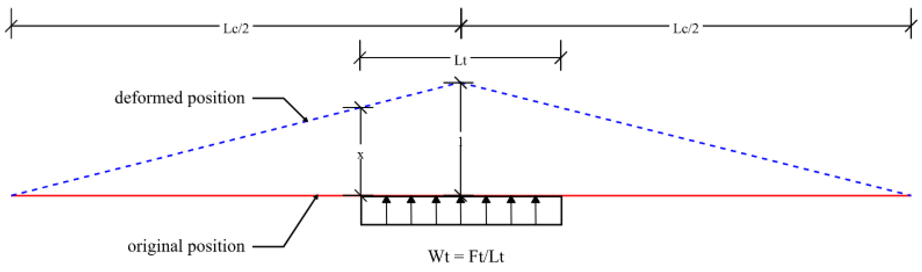
To prove the second assumption, consider a unity displacement at the top of a barrier with two slopes as shown in Figure 4. The rotation of the vertical plane is given in Equation (3).
where h1 is the total height of the barrier. The distance d1 is obtained as in Equation (4). Using the first assumption, the inextensibility of concrete, the distances d1, d2, and d3 should all be equal:
where h2 is the height of the lower part of the barrier The distances a2 and a3 are given in Equations (5) and (6).
where h3 is the height of the upper part of the barrier. The tangent of total inclination at the lower part of the barrier is given in Equation (7) as:
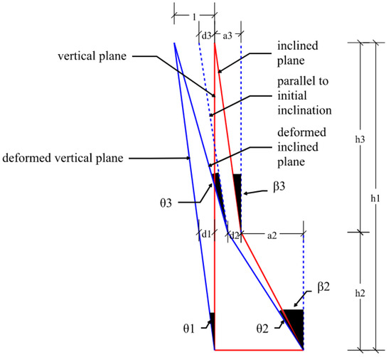
Figure 4.
Rotations of inclined planes vs. vertical planes.
Substituting the values of d2 and a2 from Equations (4) and (5) yields:
Expanding the tangent of two summed angles using trigonometric identities, and simplifying the expression gives the rotation of the lower part as in Equation (9).
Similarly, the tangent of total inclination at the upper part of the barrier is given in Equation (10) as:
Substituting the values of d3 and a3 from Equations (4) and (6) yields:
Expanding the tangent of two summed angles using trigonometric identities, and simplifying the expression gives the rotation of the upper part as in Equation (12).
It is obvious from Equations (9) and (12) that the rotation of the upper part is similar to rotation of the lower part in that they both depend on the initial inclination of the corresponding surfaces (β2 and β3). The more important observation is that when comparing Equations (3), (9) and (12) it will be obvious that the difference is due to the extra terms in the denominator. These extra terms are insignificant compared to h1. Also, since all the calculations are based on a unit deformation at the tip, which is exaggerated, the actual angle difference is even smaller in the context of small deformation theory. Therefore, the detailed YLA equations that will be derived in the coming section are based on rotations with respect to the vertical plane (θ1).
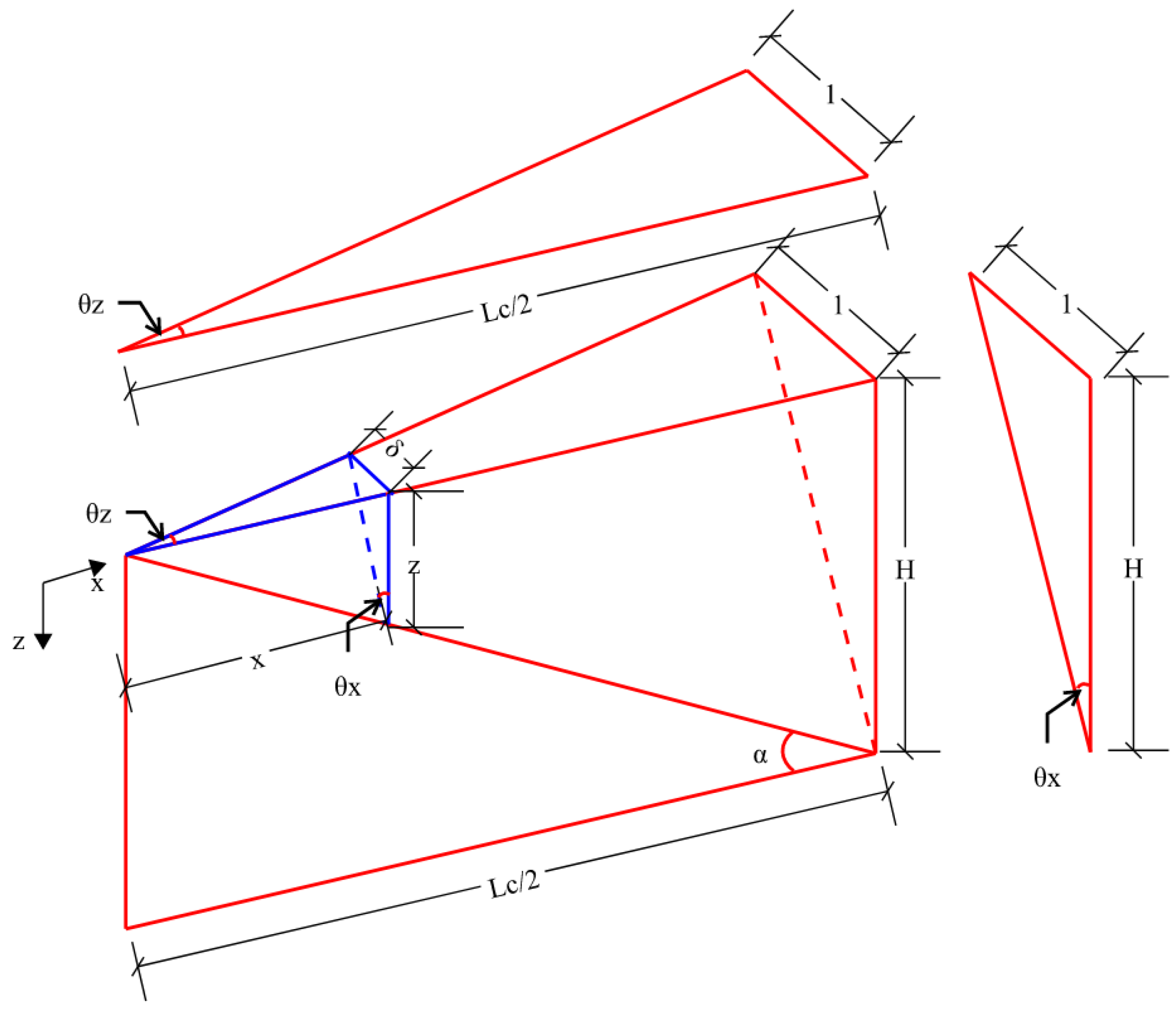
The internal work along the yield lines is the sum of the products of the yield moments and the rotations through which they act integrated along the barriers height (z-axis). The rotations correspond to Mz(z) and Mx(z) are θz(z) and θx(z) respectively as shown in Figure 5, and given by Equations (13)–(15).

Figure 5.
Formation of yield lines.
From similar triangles,
Substituting Equations (14)–(16) in Equation (13) gives:
The rotation about the horizontal axis is given as in Equation (18).
Substituting Equations (14) and (16) in Equation (18) gives:
Finally, the differential distance along an inclined yield line ds will be resolved into two components dx and dz. Since the integreations will be with respect to the depth Z, dx is given in terms of dz by differentiating Equation (15) in terms of z as in Equation (20).
3.3. Internal Work Along the Yield Lines
After obtaining the geometrical relationships of the moments and the rotations along the formed yield lines, the integrals of the internal work along the yield line at the back that is associated with two rotations around the z-axis (one rotation from each triangular piece) and the two face yield lines are given as in Equation (21).
The integration direction shown in Figure 5 will be from top to bottom for the Z-direction and from left to center for the X-direction (or right to center when considering the right segment of the barrier). That is, when , and when . Also, from Equations (17) and (19), the rotations in both directions along the yield line are constant.
Substituting Equations (17), (19) and (20) in Equation (21) gives:
3.4. External Work by Applied Loads
The length of contact between the vehicle and the concrete barrier is Lt as shown in Figure 6. Also, the force applied by the vehicle is equal to Ft. The value of Lt is specified in (Table A13.2-1) [3].
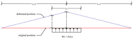
Figure 6.
Top view for vehicle-barrier contact.
The external work is given as in Equation (23).
By similar triangles the value of x can be found as:
Substituting the value of Lc from Equation (16) into Equation (24), then back into Equation (23) gives the external work as in Equation (25).
When the load acting on the barrier is concentrated at one point (the tip of the barrier), Equation (25) will become as in Equation (26).
where the load Ft is the applied concentrated load.
Equating the internal work from Equation (22) with the external work from Equation (25) or Equation (26) yields the solution for Wt and Ft as in Equation (27) and Equation (28) respectively. A closed form solution for Equations (27) and (28) can be obtained by solving respectively. Another approach is to plot their functions against a range of angles for α and selecting the minimum value of Wt in Equation (27) and Ft in Equation (28). This approach will be used in the case study section of this research.
4. Truss Analogy
One of the main contributions of this research is to propose an innovative approach for obtaining the ultimate transverse capacity of RC barriers. The approach is based on an equivalent space truss model that has properties defined to mimic the reinforcement of an actual RC barrier. This analogy is different from the AASHTO’s YLA presented in AASHTO’s YLA section in terms of relating the barrier’s capacity to the steel reinforcement only and neglecting the contribution of the concrete.
4.1. Modeling Concept
The model is based on representing the flexural capacity of the barrier about the longitudinal and vertical axes by truss elements. The profile of the truss will have the same shape as the barrier’s stirrups. The vertical framing elements of the truss will have an equal area and spacing to the existing stirrups in the actual barrier as shown in Figure 7a. The longitudinal reinforcement in the barrier is distributed on the truss elements running longitudinally, Figure 7b. Diagonal members were provided to satisfy the barrier’s ability to transfer shear forces and diagonal tension. Since the diagonals in tension carry minimal force due to concrete cracking then the diagonals in compression must be limited to concrete axial compressive strength.
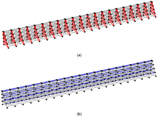
Figure 7.
Representation of the truss analogy (a) vertical frames for stirrups (b) longitudinal elements for longitudinal reinforcement.
4.2. Equivalent Failure Mechanism
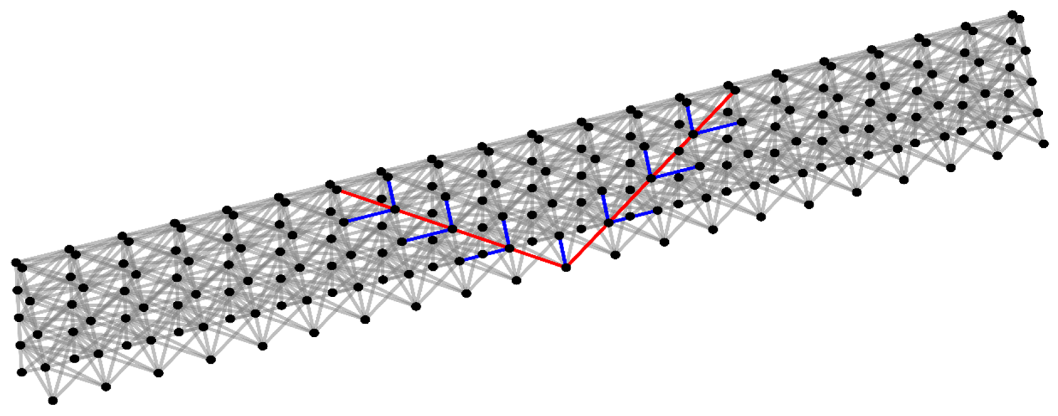
The proposed failure mechanism to simulate the failure of the barrier is by tracking the yielding of a vertical or longitudinal bar at a junction node along the first yield line as shown in Figure 8. The tracked members are the ones on the front face of the barrier and represent the two yield lines running diagonally. It is worth mentioning that by the time those two yield lines complete formation, the back yield line will be formed. Therefore, the ultimate capacity of the barrier is attached to the completion of those two yield lines. Three important aspects have been observed that are necessary to get accurate results of the barrier’s ultimate capacity by the proposed truss analogy as in the coming paragraphs.

Figure 8.
Representation of the truss analogy in terms of formation of the first yield line.
First, the analysis type needs to be nonlinear to consider the material nonlinearity of the truss elements and capture the progressive failure due to the formation of the yield lines. For this purpose, the authors developed a Python script to read the input files that contain nodes, members, boundary conditions, and loading point. The script then solves the truss using the stiffness method. The load was applied incrementally using small steps. At each load increment, all the members were checked for yielding. The yielded members will have an updated stiffness that will be used when the truss global stiffness matrix is assembled for the next loading step.
Second, the angle of the first yield line, the red line in Figure 8, varies to pick the critical angle of inclination that gives the least ultimate load. This variation is obtained through changing the distance between the vertical frames of the truss. However, varying this distance will change the configuration of the actual barrier, therefore, the stiffness of the vertical members is multiplied by a factor equals to the new spacing divided by the original spacing to maintain the same stiffness distribution of the original barrier model. This factor is sufficient to produce equivalent truss since the members’ length and orientation are not affected by the angle variation.
Finally, sizing the diagonal members is a crucial step that affects the results of ultimate capacity. The diagonal members at the back side as well as inside the truss were given a maximum strength as that of the concrete ultimate compressive strength. For the diagonal members used to track the yield line formation, the recommended approach to size them is by starting with an area equal to that of the vertical or longitudinal members, then analyzing one loading step while the structure is still all elastic. The purpose of this step is to proportion the magnitude of the load in a diagonal member with respect to the longitudinal and the vertical members that form a joint along the yield line. After that, the stresses are calculated in the vertical and longitudinal members and scaled up to the yielding stress level. Applying Mohr’s circle for the two normal stresses and rotating the angle to the desired diagonal orientation, the stress at the diagonal orientation can be found as in Equations (29)–(31). The obtained diagonal stress should be scaled up to the yielding stress by reducing the initial area of the diagonal. For more accuracy, one can repeat the elastic analysis with the updated reduced diagonal area, repeat the stress calculations, and obtain the diagonal area reduction ratio until no change in this ratio is observed.
In Equations (29)–(31), α is the angle of the desired orientation from the longitudinal direction.
In the coming section, a case study will be presented and solved by the three previously mentioned procedures. Namely, the current AASHTO’s procedure of YLA, the detailed YLA discussed in the “improved YLA of RC Barriers” section, and the truss analogy model presented in “Truss Analogy” section. The solution will be verified against numerical analysis of the barrier using Abaqus.
5. Case Study
This section will consider the Jersey barrier shown in Figure 9. The geometry was simplified by merging zones 2 and 3. The design of the barrier was provided by Kansas Department of Transportation (KDOT). The dimensions and reinforcement details are shown in Figure 9. The concrete compressive strength () is 27.6 MPa and the steel yield stress () is 413 Mpa Table 2 shows the concrete cover and rebar area information to be used in the capacity calculations.
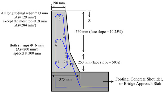
Figure 9.
Case study barrier (Jersey type).
Table 2.
Rebar layout in the barrier.
5.1. AASHTO’S Procedure of YLA
The equations provided by AASHTO Section 13 (Equations (1) and (2)) are used to calculate the lateral capacity of the barrier in this case study. The calculation process will include determining the depth of the compression block, a, per the American Concrete Institute (ACI 318) code as shown in Equation (32) [17]. After that, a weighted average is used to find the depth of the tension reinforcement, d, depending on the bars contributing to the sectional strength considered for calculations. Finally, the moment capacity of the section is found in Equation (33).
where in Equation (32): As is the area of tension steel, fy is the steel yield strength, f’c is the concrete compressive strength and b is the section width and in Equation (33): d is depth of the tension reinforcement.
For calculating Mz, the barrier was divided into two sections along its height, the first is from Z = 0 to Z = 560 mm. The second section is from Z = 560 to Z = 813 mm. Bar #3 will be considered to participate half area to the first section and half to the second section. For Mx, the moment will be calculated at the section cuts, Z = 0, Z = 560, and Z = 813 mm. It should be noted that there should be not much difference between the face and the back side moments in Mx, this is due to the approximately equal cover distance to the stirrup at both, the face and the back. The calculation of the sectional capacity per the current AASHTO’s YLA is given in Table 3.
Table 3.
Sectional capacity by AASHTO’s procedure of YLA.
According to Table A13.2-1 in Section 13 of AASHTO [3], the height of this barrier classifies as TL-4 barrier. Thus, the loading will be applied at a distributed distance of Lt = 1067 mm. Substituting the values from Table 3 in Equations (1) and (2) gives Lc = 2110 mm and Rw = 395 kN. It is worth mentioning that, according to Table A13.2-1, TL-4 barriers are required to resist a transverse load Ft of 240 kN, which this barrier satisfies. However, the coming sections will show that this is not the actual capacity of this barrier.
5.2. Improved YLA
In this section, the capacity of this barrier will be obtained through the detailed process described previously. The procedure indicated in Figure 3 will be followed in detail to find the sectional flexural capacity. According to Figure 9, there are two regions with different linear variations in terms of the depth (z). Therefore, two sections are defined to find the flexural capacity around the vertical axis (z-axis) at each side (back and front sides). Also, there are three different planes that have distinct geometry and reinforcement, the top of the barrier, the point of slope discontinuity, and the base of the barrier. Therefore, the flexural capacity around the longitudinal axis (x-axis) is represented by the capacity of these planes and will be assumed to vary linearly in between these planes. The detailed calculations of these capacities are shown in the Appendix A and summarized in Equations (34)–(36).
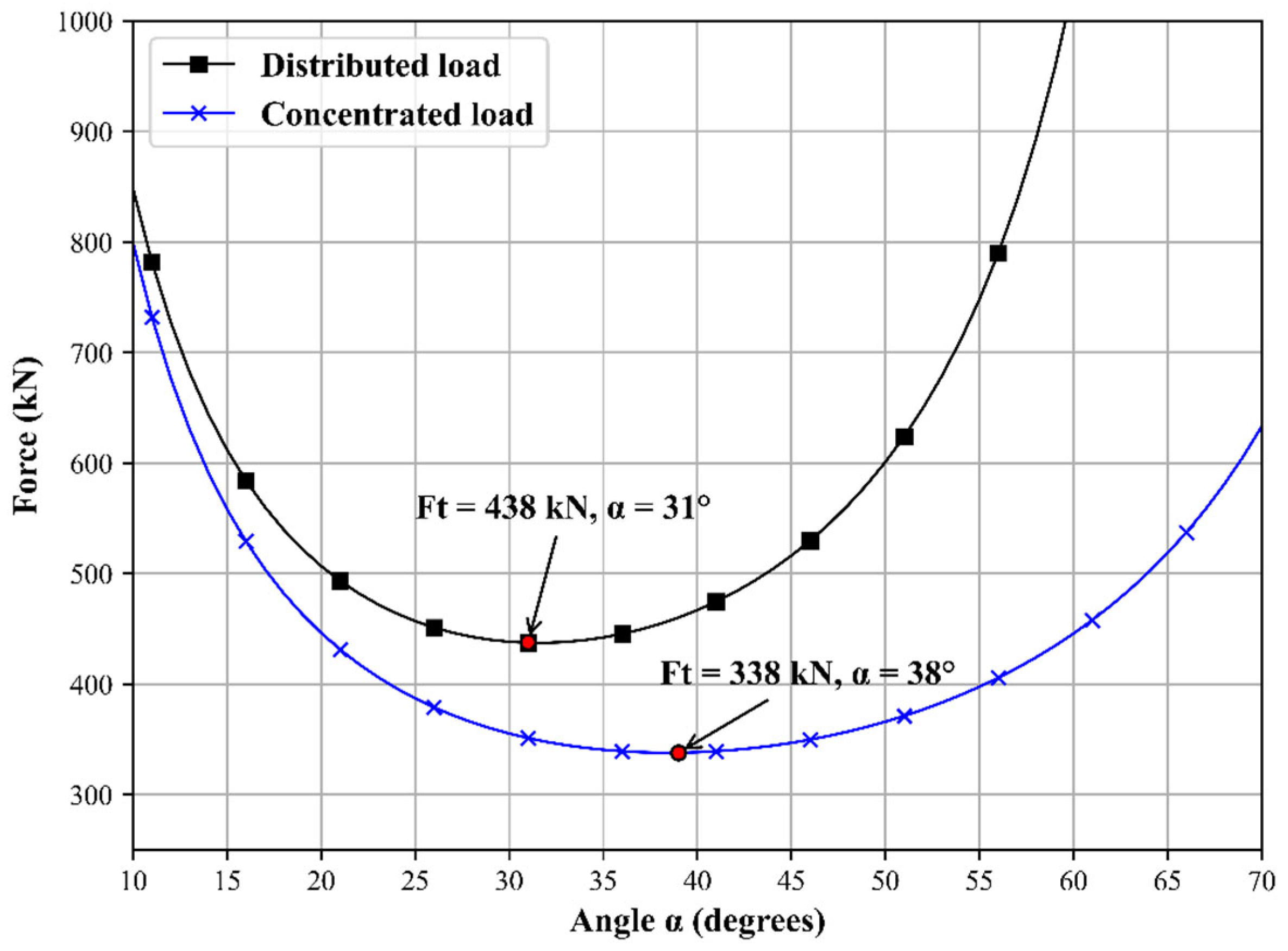
Substituting the moment functions from Equations (34)–(36) in Equation (27) for the distributed load along Lt = 1067 mm and Equation (28) for a concentrated load at the middle of the barrier gives the integration results as in Equations (37) and (38).
Solving Equations (37) and (38) for a range of angles and extracting the minimum values as in Figure 10, Equation (37) gives Wt = 0.41 N/mm, which when multiplied by Lt = 1067 mm results in a capacity Ft of 438 kN. The capacity Ft under the concentrated load, Equation (38), is 338 kN. While the concentrated load does not represent the vehicular impact force on RC barriers, it is intended to present the solution of this loading case to provide means of comparison when solving the case study using the truss analogy where the loading is concentrated at the center-upper joint.
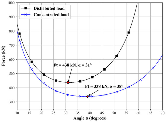
Figure 10.
Finding the critical capacity using the analytical model.
5.3. Truss Analogy
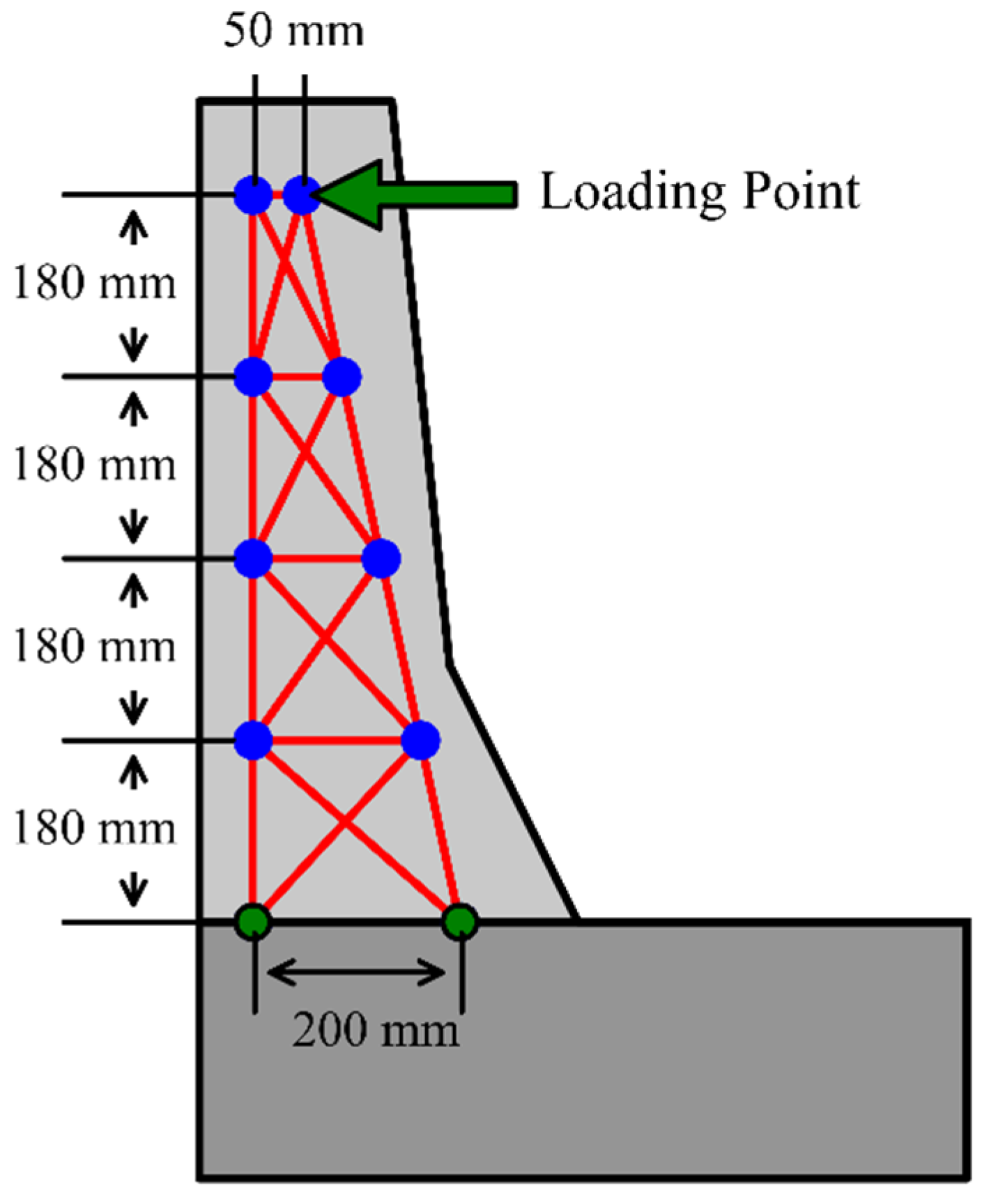
In this section, the barrier’s reinforcement is modeled as an equivalent truss structure that has similar profile shape to the stirrups’ cage shown in Figure 9. The vertical elements have an area equal to the stirrups area (200 mm2) and are spaced at 300 mm as shown in Figure 11. The longitudinal elements have an area equal to the sum of all the front side bars divided by four vertical panels, (800/4 = 200 mm2). The truss can be divided into a higher number of vertical panels along its height and yield more accurate results, however, as the number of elements increases so will the complexity of the analysis. The diagonal members at the back side as well as inside the truss were given an arbitrary area of 50 mm2 (25% of the vertical or longitudinal), but the ultimate stress in these members was set to the concrete maximum compressive strength of 27 MPa. An elastic analysis under 1 kN load step with an initial diagonal size at the front side of 200 mm2 gave vertical and longitudinal stresses of 1.865 and −0.075 MPa respectively. Scaling the higher value to the yielding stress of 413 MPa gives a scale factor of about 221 (413/1.865 = 221.4). That is, when the vertical member reaches the yielding stress of 413 MPa, the longitudinal member will have 221 times the stress of −0.075, which is −16.6 MPa. The negative value indicates that the member is under compression. The angle α is found in Equation (39).
where the 180 mm is the height of the first vertical panel, Figure 11, and the 300 mm is the spacing of the stirrups.
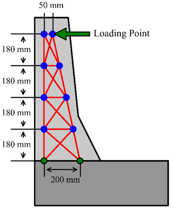
Figure 11.
Modeling barrier’s reinforcement as truss.
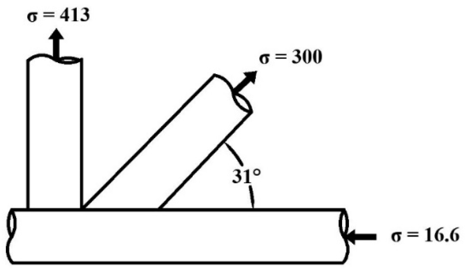
Applying Equations (29)–(31) gives a diagonal stress of 300 MPa as shown in Figure 12. Therefore, to cause yielding in the diagonal member when the vertical member starts yielding, the area of the diagonal member should be scaled down by a factor of (300/413 = 0.72), which gives an adjusted diagonal area of (0.72 × 200 = 144 mm2).

Figure 12.
Mohr’s circle stress calculation for sizing the diagonal elements.
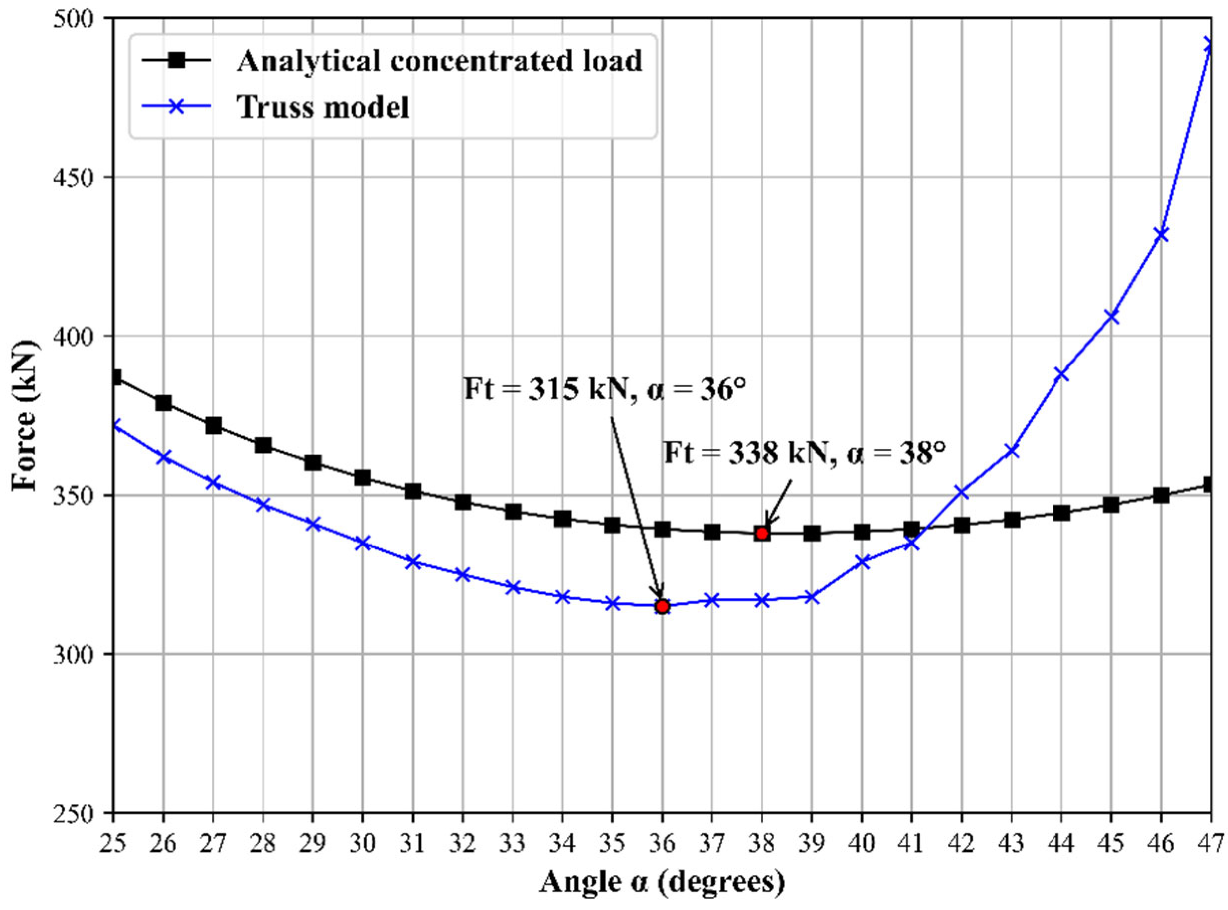
Solving the truss using incremental loading of 1 kN step for a range of α angles gives the critical load Ft that causes the truss failure according to the criteria mentioned in the Equivalent failure mechanism section, Figure 13.
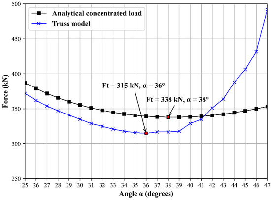
Figure 13.
Finding the critical capacity using the truss analogy model.
5.4. Finite Element Analysis by Abaqus
The final analysis method is the numerical finite element analysis (FEA) using the implicit solver of Abaqus. The model assembly consisted of the barrier (concrete) part and the reinforcement (steel) parts as shown in Figure 14.
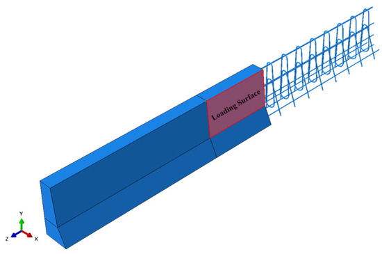
Figure 14.
Abaqus FEA model of the case study.
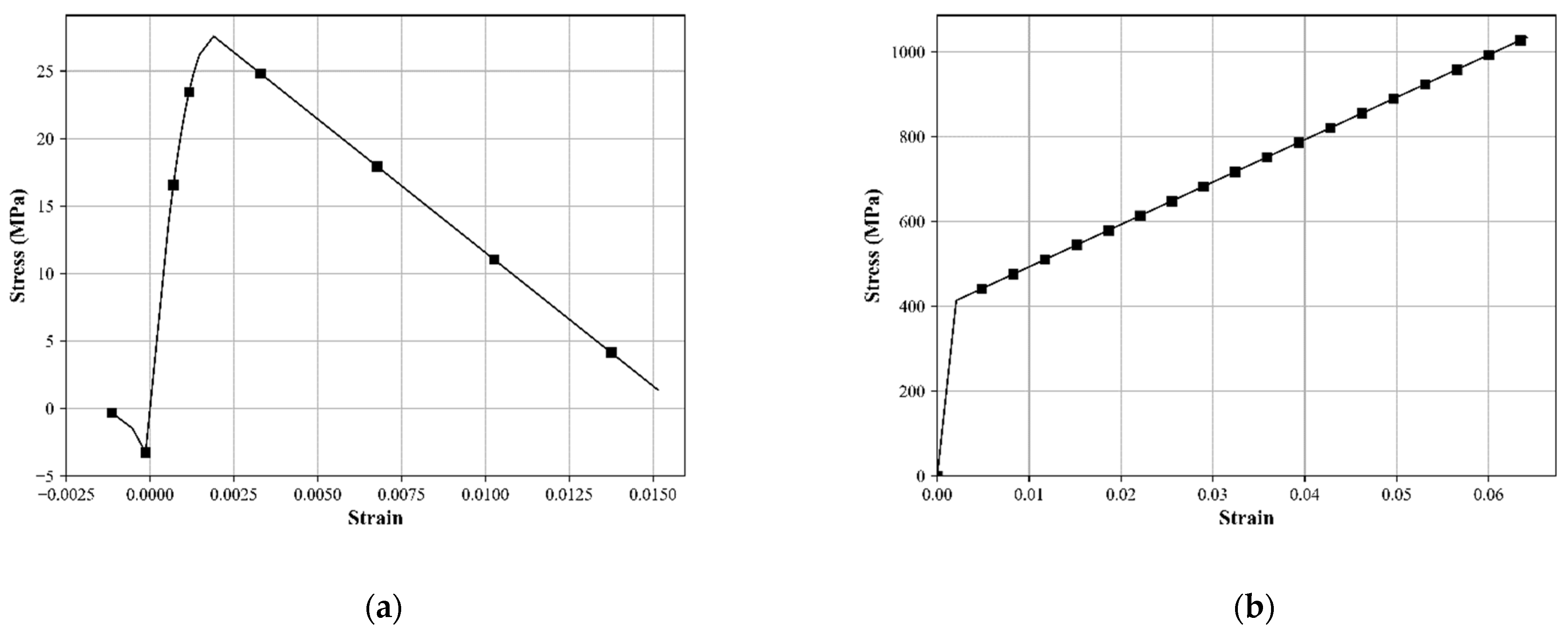
The concrete material was modeled using the concrete damage plasticity model presented in Jankowiak and Lodygowski [18] as shown in Figure 15a. The steel material was modeled bilinearly with a post yielding modulus of 5% of the initial modulus as shown in Figure 15b. The concrete elements had solid sections with an 8-node linear brick element type (C3D8R). To describe the model mesh, the largest concrete element had dimensions in mm as 60 × 60 × 40 amounting to a total of 5044 solid elements. The steel elements were modeled as beam elements with profiles corresponding to the values in Figure 9.
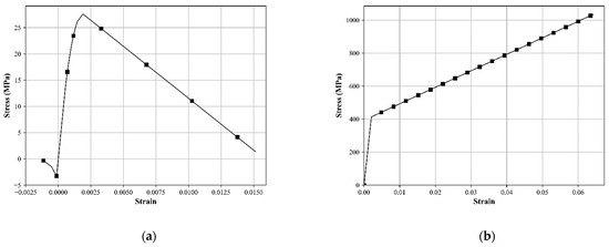
Figure 15.
Material models (a) concrete (b) steel.
The barrier’s boundary condition was fixed by restraining the translational degrees of freedom of the concrete elements at the base. The analysis type was nonlinear static Riks with the loading defined as a pressure applied at the loading surface shown in Figure 14. This surface has a length equal to 1067 mm and its width extends down until the discontinuity in the barrier’s height occurs at 560 mm. The loading surface represents the area that will come in contact with an impacting vehicle in a real crash scenario.
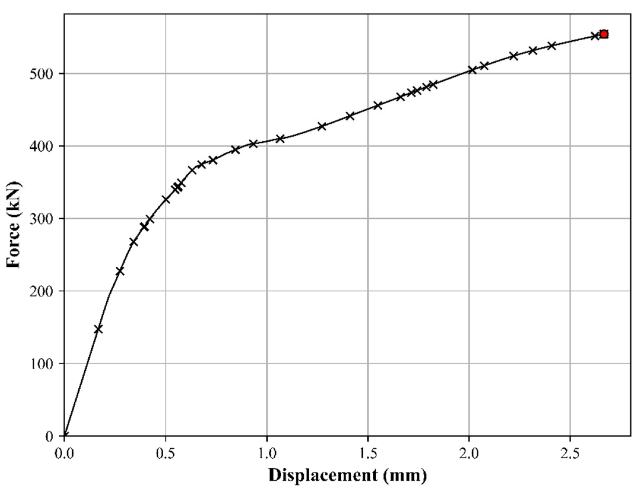
The target pressure was set to 1.72 MPa (250 psi); considering the area of pressure application, this is equvalent to a target load of 1027 kN. The analysis predicts a proportionality factor of 0.55 of the target load (1027 kN). This results in a peak capcity of 0.55 × 1027 = 554 kN as in Figure 16. The displacement in Figure 16 is measured at a node located at the middle-upper edge of the loading surface, (the middle of the entire barrier).
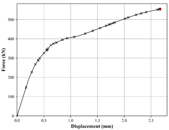
Figure 16.
FEA load-displacement response of the barrier.
Figure 17a shows the stress contour map of the barrier’s reinforcement at the peak capacity. By connecting the points of the highest stress value in each stirrup, the formation of the yield lines becomes obvious as in Figure 17a. According to the measurements shown, the angle α is calculated as 31°. The legend of the stress contour shown in Figure 17a is in psi units, the yield stress of 61,610 psi is equivalent to the 425 MPa. The model showed that yielding happened mainly in the vertical stirrups, which supports the truss analogy model. However, at the ultimate capacity of the barrier, it was observed that stirrups at higher levels did not reach complete yielding within the FEA model. This might be attributed to the failure of the concrete material that caused no further load resistance as shown in Figure 17b. The deformations in Figure 17 are magnified by 50 times.
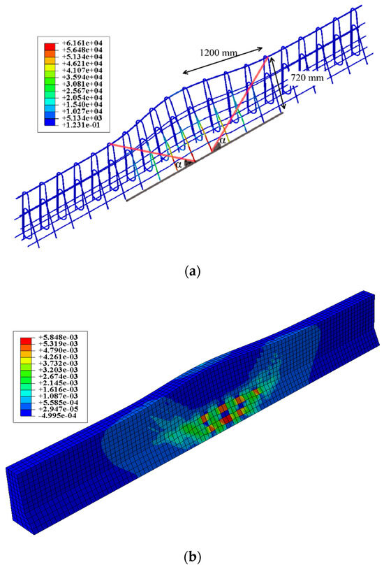
Figure 17.
(a) Stress profile in the barrier’s reinforcement (b) max. absolute principal strain in concrete.
5.5. Results Discussion
After solving the case study using the presented methods, it can be seen from Figure 10 that the ultimate capacity of the barrier when subjected to a distributed load pattern is 11% more than the capacity obtained using AASHTO’s YLA (438 to 395 kN). Also, for the analytical solution, the distributed loading pattern was about 30% higher than that of the concentrated load. This is attributed to the fact that a concentrated load will do work equal to the load multiplied by the maximum displacement assumed in the model. A uniform load is distributed over a length that varies from the same maximum displacement and other smaller ones. To produce the same work, the total of the uniform load will have to be larger in magnitude than the concentrated load. Another observation is that the range of angles providing almost the same barrier capacity was around 25–38° when the load pattern is distributed, and around 32–45° under the concentrated load effect, Figure 13. This indicates that the variation of the yield lines’ orientations within these ranges does not have major influence on the barrier’s capacity, even though it alters the range of Lc.
For the truss analogy model, the results presented in Section 5.3 show the efficiency of the proposed truss analogy model in predicting the ultimate capacity and capturing the behavior of the barrier. The comparison here is made against the analytical model of the concentrated load which is the similar loading pattern to the truss model. The differences between the two models at angles above 41° are attributed to the discrete nature of the truss. The truss model predicted the capacity of the barrier as 315 kN as compared to 338 kN by the analytical model, that is about 7% less capacity. However, the concentrated loading pattern does not represent the actual VCF, that is distributed, and the predicted value can be considered a lower bound to the limit obtained by the analytical model of the distributed load (438 kN). It can be shown from this discussion that the results of the truss analogy approach are promising and able to capture the analytical formulation.
For the FEA model, this result was about 26% larger than the analytical solution for the distributed load shown in Figure 10, (554 to 438 kN). The reason for such a difference is attributed to the strain hardening in steel that was modeled in Abaqus which starts after a capacity of about 400 kN. The YLA assumes elastic-perfectly plastic behaviour of steel. This behaviour was not considered in the numerical modeling to avoid numerical instability in the solution. Execluding the strain hardening contribution, it can be shown that the FEA and the analytical YLA are in a very good agreement, 400 kN compared to 438 kN.
6. Conclusions and Recommendations
This paper presents several methodologies for obtaining an accurate transverse capacity of RC barriers used as protective structures against VCF. The currently used AASHTO’s procedure of YLA was first discussed and the disadvantages of this procedure in term of the capacity underestimation were presented and explained. An alternative improved YLA methodology based on the same V-shape failure pattern was derived, and the procedure for implementing this methodology was explained. Furthermore, an innovative truss analogy model was proposed as a new technique for obtaining the transverse capacity of RC barriers by tracking the yielding of certain members along the anticipated yield lines. To verify the presented methodologies, a case study of an RC barrier of Jersey type was analyzed for the ultimate transverse capacity and a comparison was made. The conclusions of this study can be summarized as following:
- The current AASHTO’s YLA underestimated the barrier’s transverse capacity by about 11% and 40% compared to the detailed YLA and the FEA respectively.
- The proposed detailed YLA is powerful in obtaining the barrier’s capacity under different transverse loading patterns. A very good agreement between the capacity obtained by this method and the FEA is observed.
- The new truss analogy proposed to obtain the barrier’s transverse capacity is capable of capturing the ultimate resistance of the barrier when subjected to a transverse concentrated load. This model showed very good agreement compared to the analytical solution for the same loading pattern with some underestimation of the capacity compared to the other methods presented. Therefore, this model can be considered as a lower bound solution.
- Based on the results shown in this study, the authors recommend making a distinction in the structural adequacy criterion between the barrier’s load resistance and its geometrical adequacy to redirect colliding vehicles. The authors are currently investigating a methodology to upgrade the geometrical properties of RC barriers with innovative materials such as FRP. They conducted several studies to investigate the behavior of FRP strengthening of RC beams under dynamic load effects [19,20,21]. The current investigation considers RC barriers.
- Also, the authors recommend further development and refinement to the truss analogy model to better represent the barrier and maybe obtain the capacity under different loading patterns than the concentrated load.
Author Contributions
Conceptualization, H.A.R. and C.A.J.; methodology, H.A.R., C.A.J. and F.H.S.; software, F.H.S.; validation, H.A.R. and C.A.J.; formal analysis, F.H.S., H.A.R. and I.K.; investigation, F.H.S., H.A.R. and I.K.; resources, H.A.R. and C.A.J.; data curation, F.H.S.; writing—original draft preparation, F.H.S.; writing—review and editing, H.A.R., C.A.J. and I.K.; visualization, F.H.S.; supervision, H.A.R. and C.A.J.; project administration, H.A.R. and C.A.J.; funding acquisition, C.A.J. and H.A.R. All authors have read and agreed to the published version of the manuscript.
Funding
This research was funded by the bureau of geotechnical and structural services at Kansas Department of Transportation, grant number [K-TRAN: KSU-21-7].
Data Availability Statement
Some or all data, models, or code that support the findings of this study are available from the corresponding author upon reasonable request.
Acknowledgments
The authors would like to acknowledge the financial support for the research provided by the bureau of geotechnical and structural services at Kansas Department of Transportation through the project K-TRAN: KSU-21-7.
Conflicts of Interest
Author Fahed H. Salahat was employed by the company Stand Structural Engineering Inc. Author Isaac Klugh was employed by the company Kiewit Engineering Group Inc. The remaining authors declare that the research was conducted in the absence of any commercial or financial relationships that could be construed as a potential conflict of interest.
Appendix A
Table A1.
Back side sectional capacity around the vertical axis.
Table A1.
Back side sectional capacity around the vertical axis.
| Back Side | ||
|---|---|---|
| Step | Section 1 (Z1 = 0–560) | Section 2 (Z2 = 560–813) |
| 1 | ||
| 2 | ||
| 3 | ||
| 4 | ||
| 5 | ||
Table A2.
Front side sectional capacity around the vertical axis.
Table A2.
Front side sectional capacity around the vertical axis.
| Front Side | ||
|---|---|---|
| Step | Section 1 (Z1 = 0–560) | Section 2 (Z2 = 560–813) |
| 1 | ||
| 2 | ||
| 3 | ||
| 4 | ||
| 5 | ||
Table A3.
Face side sectional capacity around the longitudinal axis.
Table A3.
Face side sectional capacity around the longitudinal axis.
| Step | Front Side | ||
|---|---|---|---|
| 1 | Section 1 (Z1 = 0 mm) | Section 2 (Z2 = 560 mm) | Section 3 (Z3 = 813 mm) |
| 2 | |||
| 3 | |||
| 4 | |||
| 5 | |||
References
- Ross, H.E. (Ed.) Recommended procedures for the safety performance evaluation of highway features. In National Cooperative Highway Research Program Report; no. 350; Transportation Research Board, National Research Council; National Academy Press: Washington, DC, USA, 1993; ISBN 978-0-309-04873-6. [Google Scholar]
- American Association of State Highway and Transportation Officials. Manual for Assessing Safety Hardware, 2nd ed.; American Association of State Highway and Transportation Officials: Washington, DC, USA, 2016; ISBN 978-1-56051-665-1. [Google Scholar]
- American Association of State Highway and Transportation Officials. LRFD Bridge Design Specifications; American Association of State Highway and Transportation Officials: Washington, DC, USA, 2020; ISBN 978-1-56051-738-2. [Google Scholar]
- Hirsch, T.J. Analytical Evaluation of Texas Bridge Rails to Contain Buses and Trucks. Art. no. FHWATX78-230–2. August 1978. Available online: https://trid.trb.org/view/138035 (accessed on 30 January 2023).
- Jeon, S.-J.; Choi, M.-S.; Kim, Y.-J. Ultimate Strength of Concrete Barrier by the Yield Line Theory. Int. J. Concr. Struct. Mater. 2008, 2, 57–62. [Google Scholar] [CrossRef]
- Cao, R.; Agrawal, A.K.; El-Tawil, S.; Wong, W. Numerical Studies on Concrete Barriers Subject to MASH Truck Impact. J. Bridge Eng. 2020, 25, 04020035. [Google Scholar] [CrossRef]
- Loken, A.E.; Steelman, J.S.; Rosenbaugh, S.K.; Faller, R.K.; Holt, J.M. Comparison of Modified Yield-Line and Punching Shear Capacities for Concrete Traffic Barriers and Bridge Rails. Transp. Res. Rec. 2021, 2675, 689–701. [Google Scholar] [CrossRef]
- Alberson, D.C.; Williams, W.F.; Menges, W.L. Testing and Evaluation of the Florida F Shape Bridge Rail with Reduced Deck Thickness; FHWA/TX-05/9-8132-3; Texas Dept. of Transportation: College Station, TX, USA, 2005. [Google Scholar]
- Williams, W.F.; Buth, C.E.; Menges, W.L. Repair/Retrofit Anchorage Designs for Bridge Rails; Texas A&M Transportation Institute: College Station, TX, USA, 2007. [Google Scholar]
- Sennah, K.; Tropynina, E.; Ibrahim, Z.; Hedjazi, S. Structural qualification of a developed GFRP-reinforced concrete bridge barrier using ultimate load testing. Int. J. Concr. Struct. Mater. 2018, 12, 63. [Google Scholar]
- Rosenbaugh, S.; Sicking, D.; Faller, R. Development of a TL-5 Vertical Faced Concrete Median Barrier Incorporating Head Ejection Criteria. Neb. Dep. Transp. Res. Rep. 2007. Available online: https://digitalcommons.unl.edu/ndor/38 (accessed on 30 March 2025).
- Bullard, D.; Roger, P.B.; Menges, W.L.; Haug, R.R. Evaluation of Existing Roadside Safety Hardware Using Updated Criteria Technical Report (2010); Transportation Research Board: Washington, DC, USA, 2010; Volume 1, p. 22938. ISBN 978-0-309-43011-1. [Google Scholar]
- Salahat, F.H.; Jones, C.A.; Rasheed, H.A. Estimation of Vehicular Collision Force on Bridge Piers in the Presence of Sub-Standard Intervening Concrete Barriers. Transp. Res. Rec. 2023, 2677, 326–339. [Google Scholar] [CrossRef]
- Salahat, F.H. Performance of Sub-Standard Reinforced Concrete Barriers in Protecting Bridge Piers Against Vehicular Collision Force. 2023. Available online: https://krex.k-state.edu/items/bd143abd-bd70-4c89-97f7-17578cce6728 (accessed on 30 March 2025).
- Salahat, F.H.; Jones, C.A.; Rasheed, H.A. Assessment of Substandard Concrete Barriers as Protective Structures to Bridge Piers against Vehicular Collision Force. J. Bridge Eng. 2024, 29, 04024043. [Google Scholar] [CrossRef]
- Kim, J.J.; Ahn, J.S. Vehicle Collision Analysis of the Reinforced Concrete Barriers Installed on Bridges Using Node-Independent Model. Appl. Sci. 2024, 14, 10518. [Google Scholar] [CrossRef]
- Building Code Requirements for Structural Concrete (ACI 318-25) and Commentary on Building Code Requirements for Structural Concrete (ACI 318R-25); American Concrete Institute: Farmington Hills, MI, USA, 2025.
- Jankowiak, T.; Lodygowski, T. Identification of parameters of concrete damage plasticity constitutive model. Found. Civ. Environ. Eng. 2005, 6, 53–69. [Google Scholar]
- Alshamrani, S.; Salahat, F.; Rasheed, H.; Shapack, G.; Albahttiti, M. Cyclic Performance of Carbon Fiber-Re info reed Polymer-Strengthened Reinforced Concrete Beams in Flexure. ACI Struct. J. 2025, 122, 161–174. [Google Scholar]
- Alshamrani, S.; Saleem, S.M.; Rasheed, H.A.; Salahat, F.H. Salahat Modeling Cyclic Response of CFRP Strengthened Fiber Anchored RC Frame Members to Failure. ACI Symp. Publ. 2024, 360. Available online: https://www.concrete.org/publications/internationalconcreteabstractsportal/m/details/id/51740641 (accessed on 30 March 2025).
- Alshamrani, S.; Rasheed, H.A.; Salahat, F.H.; Borwankar, A.; Divilbiss, N. Seismic flexural behavior of CFRP strengthened reinforced concrete beams secured with fiber anchors. Eng. Struct. 2024, 305, 117728. [Google Scholar] [CrossRef]


Disclaimer/Publisher’s Note: The statements, opinions and data contained in all publications are solely those of the individual author(s) and contributor(s) and not of MDPI and/or the editor(s). MDPI and/or the editor(s) disclaim responsibility for any injury to people or property resulting from any ideas, methods, instructions or products referred to in the content. |
© 2025 by the authors. Licensee MDPI, Basel, Switzerland. This article is an open access article distributed under the terms and conditions of the Creative Commons Attribution (CC BY) license (https://creativecommons.org/licenses/by/4.0/).