
Modeling and Classification of Random Traffic Patterns for Fatigue Analysis of Highway Bridges


 ,
,
Abstract
1. Introduction
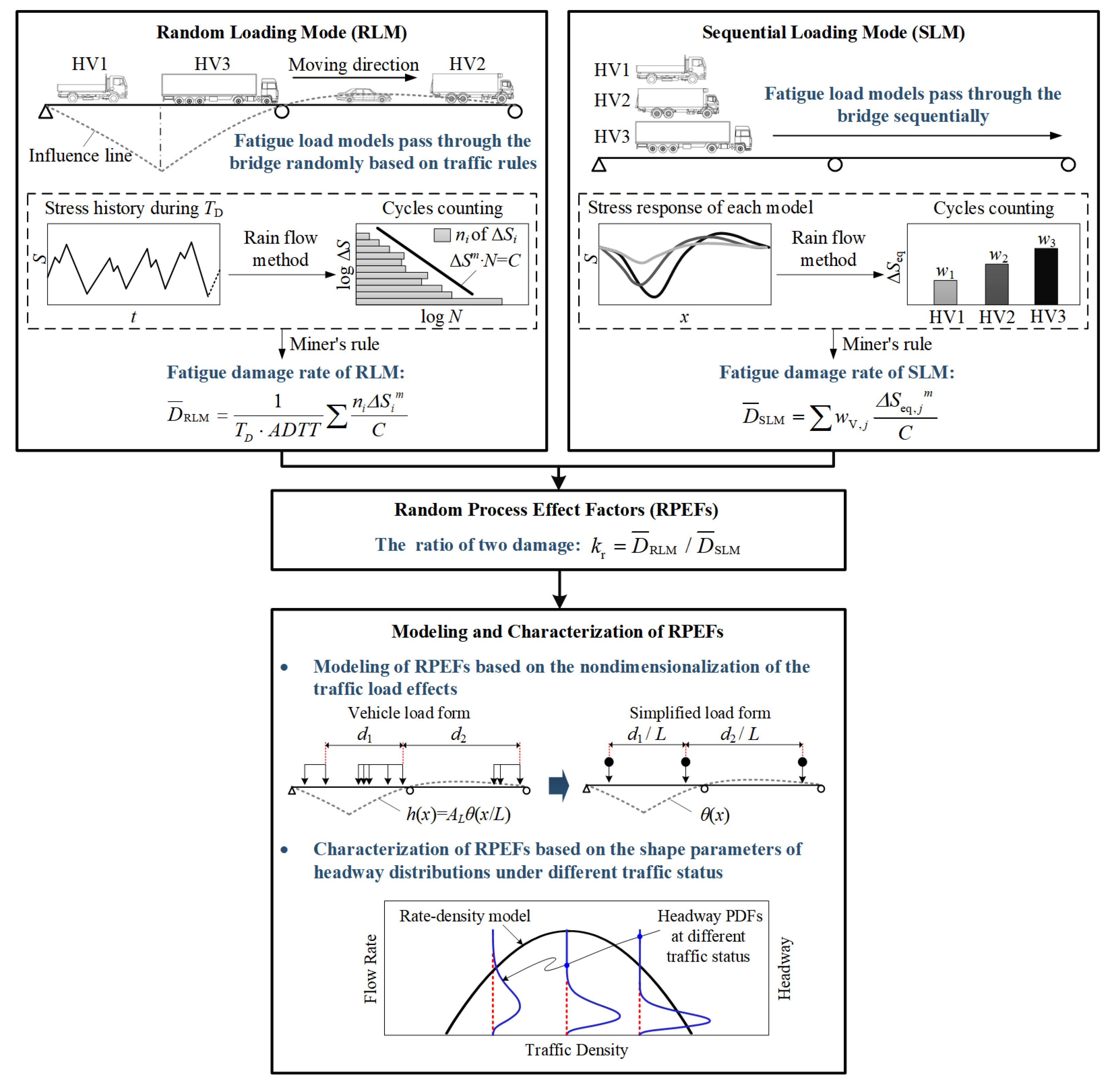
2. Concept and Framework
3. Modeling of RPEFs
3.1. Similarity Principle of Filtered Stochastic Processes and Its Inference
3.2. Functional Form of RPEFs and Its Limits
4. Numerical Analysis of RPEFs
4.1. Objectives and Solutions
4.2. Simulation Parameters
- (1)
- Fatigue load spectrum
- (2)
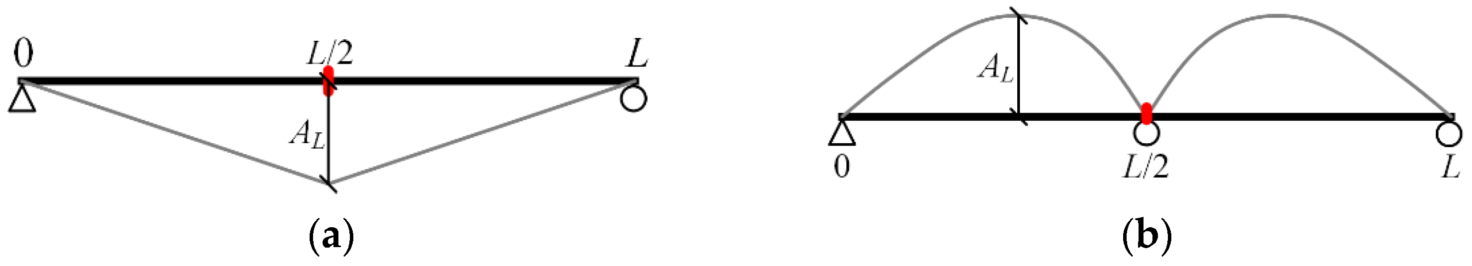
- Influence lines
- (3)
- S–N curve type
- (4)
- Vehicle headway distributions
- (5)
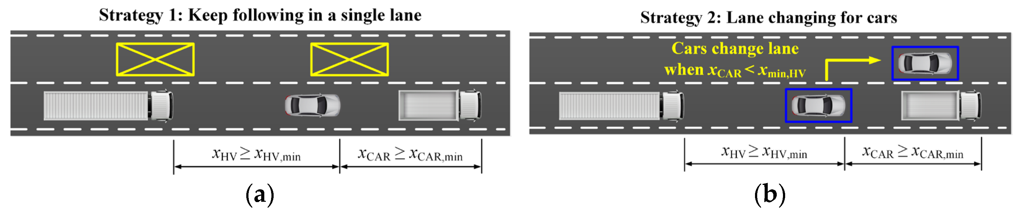
- Vehicle minimum driving spacing
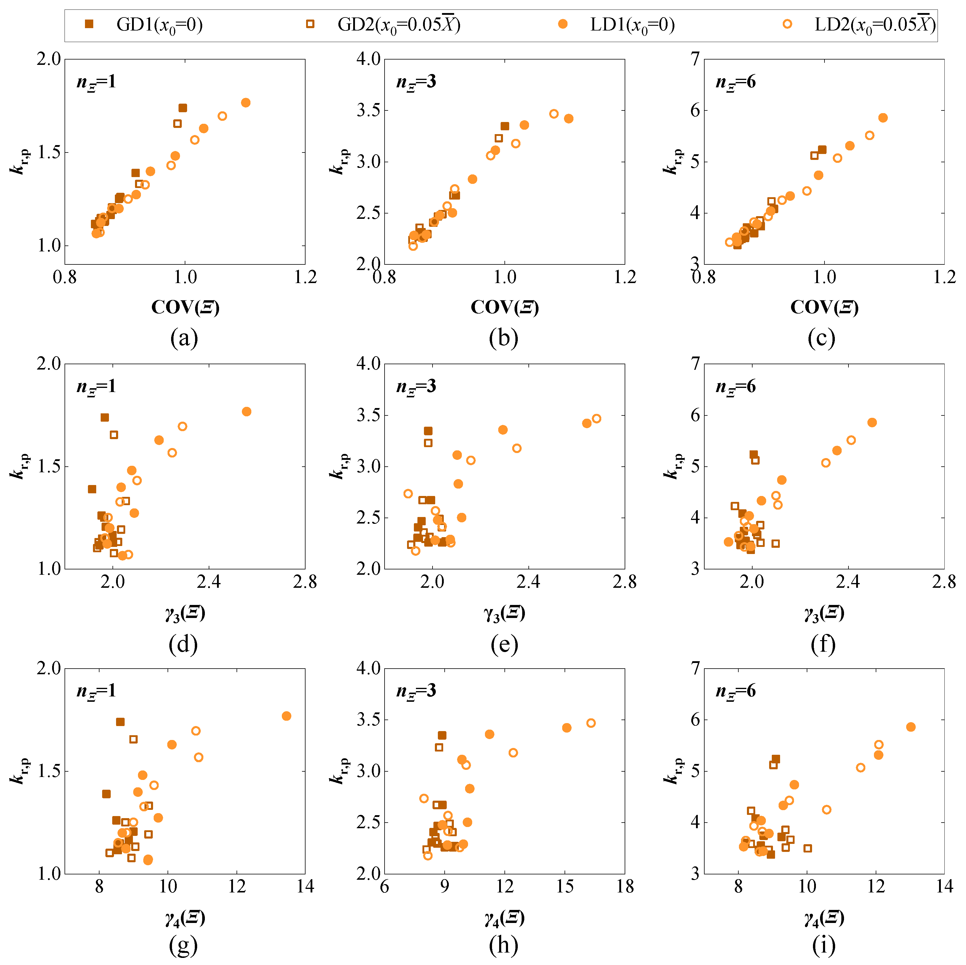
4.3. Shape Effects of Arrival Probability Model
4.4. Cluster Analysis of RPEFs Under Macroscopic Traffic Flow
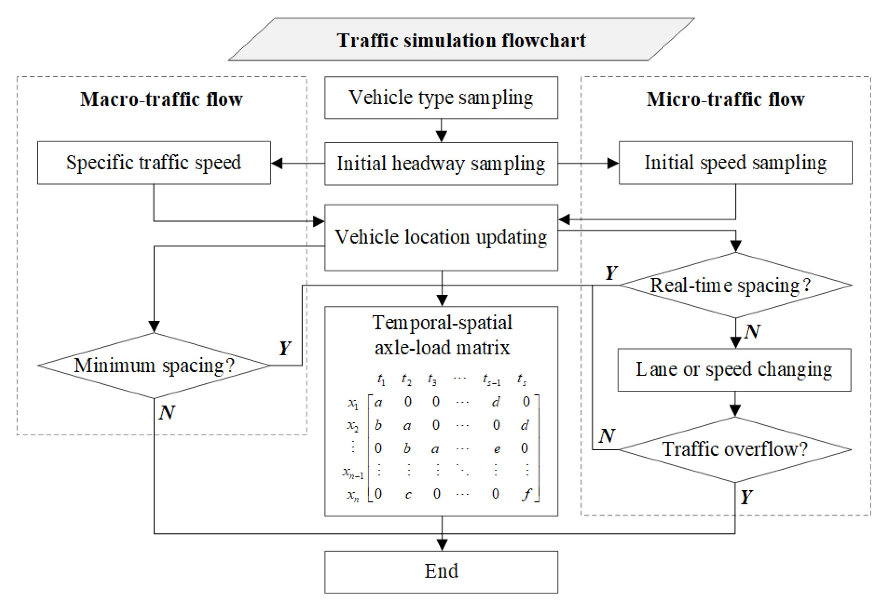
4.5. The Impact of Microscopic Traffic Behavior on RPEFs
5. Fatigue Damage Assessment Under Mixed Traffic Conditions
5.1. Equivalent RPEFs
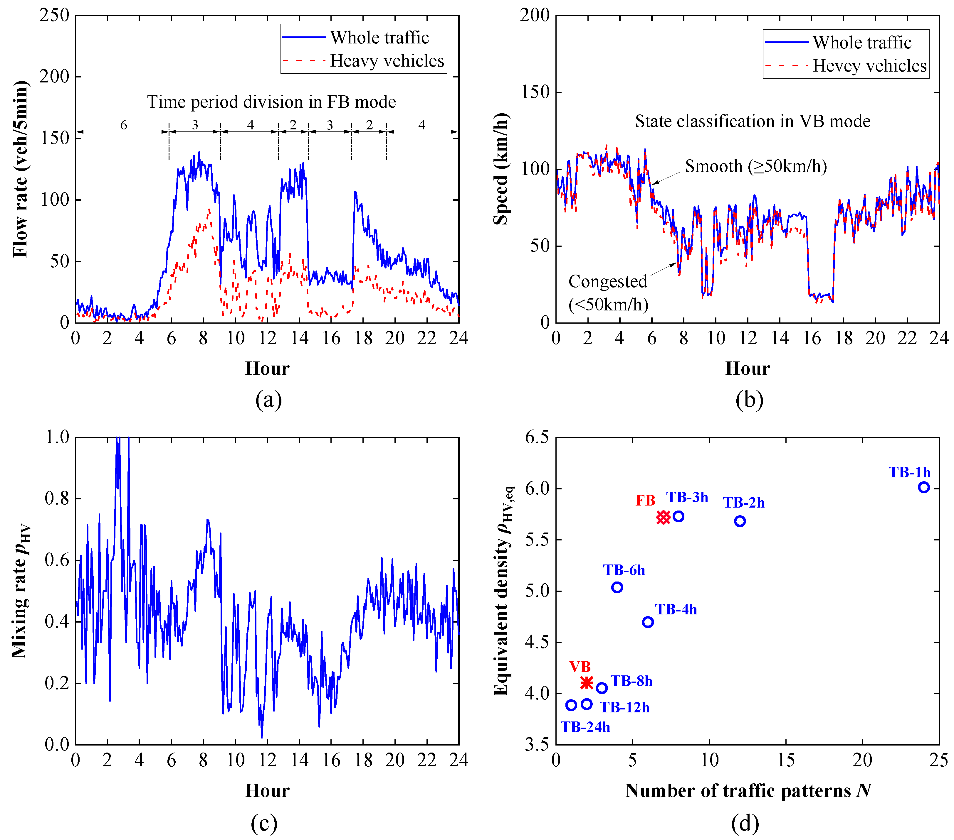
5.2. Optimization of Traffic Pattern Classification
5.3. Case Study
6. Conclusions
Author Contributions
Funding
Data Availability Statement
Acknowledgments
Conflicts of Interest
Abbreviations and Nomenclature
| CAFL | Constant Amplitude Fatigue Limit |
| COV | Coefficient of Variation |
| GVW | Gross Vehicle Weight |
| PRLM | Point Random Loading Mode |
| RPEF | Random Process Effect Factor |
| RLM | Random Loading Mode |
| SLM | Sequential Loading Mode |
| average fatigue damage per vehicle under RLM | |
| average fatigue damage per vehicle under SLM | |
| HD | spatial headway |
| HT | temporal headway |
| HHV | headway of heavy vehicle traffic |
| HW | headway of whole traffic |
| L | bridge length |
| kr | random process effect factor (damage ratio of and ) |
| kr,p | random process effect factor under point loading mode |
| kr,eq | equivalent random process effect factor under mixed traffic conditions |
| nΞ | average occurrence of vehicle loads on bridge |
| λHV | traffic density of heavy vehicle traffic |
| λW | traffic flow rate of traffic as a whole |
| ρHV | traffic density of heavy vehicle traffic |
| ρW | traffic density of traffic as a whole |
| ρHV,eq | equivalent traffic density of all traffic under mixed traffic conditions |
Appendix A
- (1)
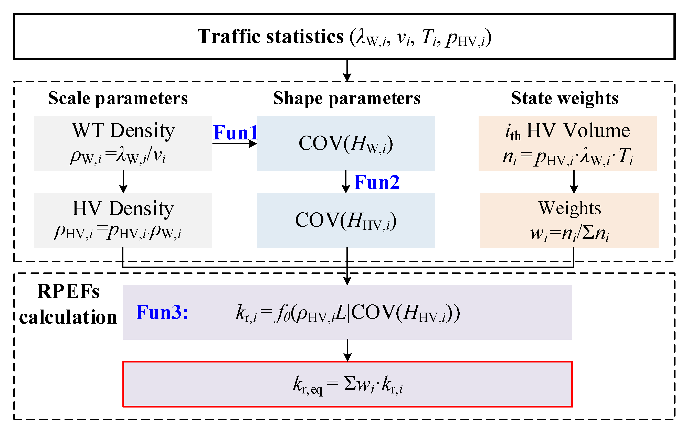
- Fun1 is a functional relationship between the coefficient of variation of headway COV(HW) and the traffic density ρW of the whole traffic flow. It is the fitted curve in Figure 13a with a correlation coefficient R2 = 0.83, and the expression is
- (2)
- Fun2 is a functional relationship between the coefficient of variation of heavy vehicle headway COV(HHV), the coefficient of variation of whole traffic headway COV(HW), and the heavy vehicle mixing ratio pHV. They are the fitted curves in Figure 13b with a correlation coefficient R2 = 0.80, and the expression is
- (3)
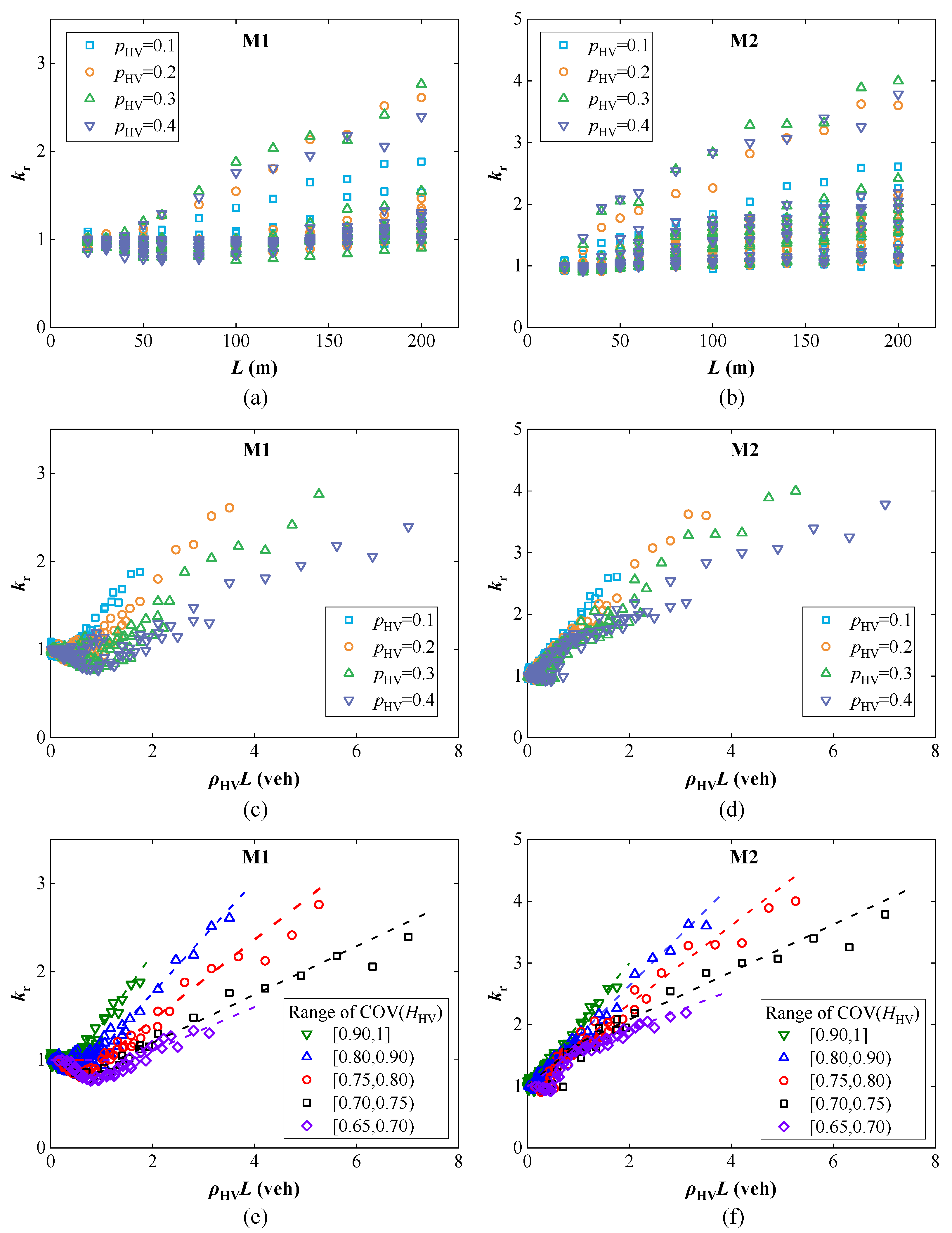
- Fun3 is a calibration curve for the kr coefficient (Figure 8e,f), developed based on classification according to influence lines and COV(HHV). Due to significant differences in trends among traffic states, Fun3 is formulated uniformly as segmented straight lines, providing the starting coordinates for each segment curve and the slope between each point. For example, (A1, B1)-K1-(A2, B2)-K2, where the starting coordinates for the first segment are (A1, B1), and for the second segment are (A2, B2). K1 represents the slope between (A1, B1) and (A2, B2) (where, K1 = (B2 - B1)/(A2 - A1)), and K2 is the slope after (A2, B2). This allows for the determination of the kr value at any point on this curve.

| Influence Line | Interval of COV(HHV) | Coordinates and Slopes |
|---|---|---|
| M1 | [0.90, 1.0] | (0, 1)-0-(0.5, 1)-0.8 |
| [0.80, 0.90) | (0, 1)-0-(0.8, 1)-0.633 | |
| [0.75, 0.80) | (0, 1)-0-(1, 1)-0.455 | |
| [0.70, 0.75) | (0, 1)-0-(1.3, 1)-0.275 | |
| [0.65, 0.70) | (0, 1)-0-(1.6, 1)-0.25 | |
| M2 | [0.90, 1.0] | (0, 1)-1 |
| [0.80, 0.90) | (0, 1)-0.816 | |
| [0.75, 0.80) | (0, 1)-0.715-(0.7, 1.5)-0.639 | |
| [0.70, 0.75) | (0, 1)-0.7-(1, 1.7)-0.385 | |
| [0.65, 0.70) | (0, 1)-0.6-(1, 1.6)-0.319 |
References
- AASHTO. AASHTO LRFD Bridge Design Specifications, 9th ed.; American Association of State Highway and Transportation Officials, Inc.: Washington, DC, USA, 2020. [Google Scholar]
- CEN. Eurocode 3: Design of Steel Structures-Part 2: Steel Bridges; European Committee for Standardization: Brussels, Belgium, 2006. [Google Scholar]
- SIA. SIA 263: Steel Construction; Swiss Society of Engineers and Architects: Zurich, Switzerland, 2003. [Google Scholar]
- Wang, Z.W.; Zhang, W.M.; Zhang, Y.F.; Liu, Z. Temperature prediction of flat steel box girders of long-span bridges utilizing in situ environmental parameters and machine learning. J. Bridge Eng. 2022, 27, 04022004. [Google Scholar] [CrossRef]
- Ding, Y.; Ye, X.W.; Su, Y.H. Wind-induced fatigue life prediction of bridge hangers considering the effect of wind direction. Eng. Struct. 2025, 327, 119523. [Google Scholar] [CrossRef]
- Dan, D.; Ying, Y.; Ge, L. Digital twin system of bridges group based on machine vision fusion monitoring of bridge traffic load. IEEE Trans. Intell. Transp. 2021, 23, 22190–22205. [Google Scholar] [CrossRef]
- Zhang, H.; Shen, M.; Zhang, Y.; Chen, Y.; Lü, C. Identification of static loading conditions using piezoelectric sensor arrays. Int. J. Appl. Mech. 2018, 85, 011008. [Google Scholar] [CrossRef]
- Huang, K.; Zhang, H.; Jiang, J.; Zhang, Y.; Zhou, Y.; Sun, L.; Zhang, Y. The optimal design of a piezoelectric energy harvester for smart pavements. Int. J. Mech. Sci. 2022, 232, 107609. [Google Scholar] [CrossRef]
- Chen, B.; Li, X.; Xie, X.; Zhong, Z.; Lu, P. Fatigue performance assessment of composite arch bridge suspenders based on actual vehicle loads. Shock Vib. 2015, 2015, 659092. [Google Scholar] [CrossRef]
- Ravichandran, N.; Losanno, D.; Pecce, M.R.; Parisi, F. Site-specific traffic modelling and simulation for a major Italian highway based on weigh-in-motion systems accounting for gross vehicle weight limitations. J. Civ. Struct. Health 2024, 14, 1739–1763. [Google Scholar] [CrossRef]
- Zhou, J.; Caprani, C.C.; Zhang, L. On the structural safety of long-span bridges under traffic loadings caused by maintenance works. Eng. Struct. 2021, 240, 112407. [Google Scholar] [CrossRef]
- Yang, D.H.; Guan, Z.X.; Yi, T.H.; Li, H.N.; Ni, Y.S. Fatigue evaluation of bridges based on strain influence line loaded by elaborate stochastic traffic flow. J. Bridge Eng. 2022, 27, 04022082. [Google Scholar] [CrossRef]
- Bruls, A.; Croce, P.; Sanpaolesi, L.; Sedlacek, G. ENV 1991-Part 3: Traffic loads on bridges: Calibration of road load models for road bridges. IABSE Colloq. Basis Des. Actions Struct. 1996, 74, 439–453. [Google Scholar]
- Nussbaumer, A.; Oliveira Pedro, J.; Pereira Baptista, C.A.; Duval, M. Fatigue Damage Factor Calibration for Long-Span Cable-stayed Bridge Decks. In Mechanical Fatigue of Metals: Experimental and Simulation Perspectives; Springer Nature: Cham, Switzerland, 2019; Volume 7, pp. 369–376. [Google Scholar]
- Maljaars, J. Evaluation of traffic load models for fatigue verification of European road bridges. Eng. Struc. 2020, 225, 111326. [Google Scholar] [CrossRef]
- Baptista, C. Multiaxial and Variable Amplitude Fatigue in Steel Bridges. Ph.D. Thesis, Swiss Federal Institute of Technology in Lausanne (EPFL), Lausanne, Switzerland, 2016. [Google Scholar]
- Wysokowski, A. Impact of traffic load randomness on fatigue of steel bridges. Balt. J. Road Bridge Eng. 2020, 15, 21–44. [Google Scholar] [CrossRef]
- Maddah, N.; Nussbaumer, A. Evaluation of Eurocode damage equivalent factor based on traffic simulation. In Proceedings of the 6th International Conference on Bridge Maintenance, Safety and Management, Milan, Italy, 8–12 July 2012. [Google Scholar]
- Maddah, N. Fatigue Life Assessment of Roadway Bridges Based on Actual Traffic Loads. Ph.D. thesis, Swiss Federal Institute of Technology in Lausanne (EPFL), Lausanne, Switzerland, 2013. [Google Scholar]
- Walbridge, S.; Fischer, V.; Maddah, N.; Nussbaumer, A. Simultaneous vehicle crossing effects on fatigue damage equivalence factors for North American roadway bridges. J. Bridge Eng. 2013, 18, 1309–1318. [Google Scholar] [CrossRef]
- Moghimi, H.; Ronagh, H.R. Impact factors for a composite steel bridge using non-linear dynamic simulation. Int. J. Impact Eng. 2008, 35, 1228–1243. [Google Scholar] [CrossRef]
- Xie, X.; Wu, D.; Zhang, H.; Shen, Y.; Mikio, Y. Low-frequency noise radiation from traffic-induced vibration of steel double-box girder bridge. J. Vib. Control 2012, 18, 373–384. [Google Scholar] [CrossRef]
- Shinozuka, M.; Matsumura, S.; Kubo, M. Analysis of highway bridge response to stochastic live loads. Doboku Gakkai Ronbunshu 1984, 1984, 367–376. [Google Scholar] [CrossRef]
- Okabayashi, T.; Yamate, H. Analysis of highway bridge response to stochastic traffic flows using non-gaussian process. Rep. Fac. Eng. Nagasaki Univ. 1985, 15, 53–60. [Google Scholar]
- Forbes, C.; Evans, M.; Hastings, N.; Peacock, B. Statistical Distributions; John Wiley & Sons, Inc.: Hoboken, NJ, USA, 2011. [Google Scholar]
- May, A.D. Traffic Flow Fundamentals; Prentice Hall: Upper Saddle River, NJ, USA, 1990. [Google Scholar]
- Chen, B.; Zhong, Z.; Xie, X.; Lu, P. Measurement-based vehicle load model for urban expressway bridges. Math. Probl. Eng. 2014, 2014, 340896. [Google Scholar] [CrossRef]
- JSSC. Recommendations for Fatigue Design of Steel Structures; Japanese Society of Steel Construction: Tokyo, Japan, 1995. [Google Scholar]
- Leonetti, D.; Maljaars, J.; Snijder, H.H. Probabilistic fatigue resistance model for steel welded details under variable amplitude loading–Inference and uncertainty estimation. Int. J. Fatigue 2020, 135, 105515. [Google Scholar] [CrossRef]
- CEN. Eurocode 3: Design of Steel Structures, Part 1-9: Fatigue; European Committee for Standardization: Brussels, Belgium, 2005. [Google Scholar]
- Zheng, X.; Zhang, H.; Shen, M.; Xie, X. Research on calibration strategy of damage equivalence factor based on critical resistance analysis indexes for road steel bridges. China Civ. Eng. J. 2023, 56, 32–42. [Google Scholar]
- Xiang, Q.; Wang, W.; Li, W. A Study on the Vehicle Minimum Time Headway. J. Southeast. Univ. 1998, 28, 79–82. [Google Scholar]
- Chen, S.R.; Wu, J. Modeling stochastic live load for long-span bridge based on microscopic traffic flow simulation. Comput. Struct. 2011, 89, 813–824. [Google Scholar] [CrossRef]
- Li, Y.; Bao, W.; Guo, X. Reliability and Probability-Based Limit State Design of Highway Bridge Structures; China Communications Press: Beijing, China, 1997. [Google Scholar]
- Maurya, A.K.; Dey, S.; Das, S. Speed and time headway distribution under mixed traffic condition. J. East. Asia Soc. Transp. Stud. 2015, 11, 1774–1792. [Google Scholar]
- Abtahi, S.M.; Tamannaei, M.; Haghshenash, H. Analysis and modeling time headway distributions under heavy traffic flow conditions in the urban highways: Case of Isfahan. Transport 2011, 26, 375–382. [Google Scholar] [CrossRef]
- Yin, S.; Li, Z.; Zhang, Y.; Yao, D.; Su, Y.; Li, L. Headway distribution modeling with regard to traffic states. In Proceedings of the 2009 IEEE Intelligent Vehicles Symposium, Xi’an, China, 3–5 June 2009. [Google Scholar]
- Chen, X. Modeling Traffic Flow Dynamic and Stochastic Evolutions. Ph.D. Thesis, Tsinghua University, Beijing, China, 2012. [Google Scholar]


| Heavy Vehicle Type | Percentage (%) | Average Axle Weight (tf) and Axle Spacing (m) | |
|---|---|---|---|
| V21 |  | 8.75 | 1.89 (3.0) 2.3 |
| V22 | 45.11 | 3.40 (4.7) 7.74 | |
| V23 | 30.30 | 5.05 (6.6) 9.84 | |
| V31 |  | 2.79 | 4.36 (2.1) 4.48 (5.8) 1.37 |
| V32 |  | 3.09 | 7.68 (5.0)13.66 (1.5) 13.74 |
| V41 |  | 4.59 | 6.85 (2.0) 7.44 (4.8) 13.97 (1.4) 15.25 |
| V42 |  | 1.82 | 4.1 (3.8) 12.03 (6.8) 11.96 (1.4) 11.87 |
| V51 |  | 1.74 | 5.55 (3.7) 12.53 (6.6) 11.47 (1.4) 10.75 (1.4) 11.23 |
| V61 |  | 1.03 | 4.24 (1.9) 4.4 (2.7) 11.29 (6.6) 9.61 (1.4) 9.71 (1.4) 10.49 |
| V62 |  | 0.78 | 5.59 (3.5) 8.42 (1.5) 7.98 (7.0) 9.59 (1.4) 9.24 (1.4) 10.3 |
| Heavy Vehicle Type | Distribution Type | First Distribution | Second Distribution | Third Distribution | ||||||
|---|---|---|---|---|---|---|---|---|---|---|
| p1 | μ1 | σ1 | p2 | μ2 | σ2 | p3 | μ3 | σ3 | ||
| V21 | Lognormal | 0.35 | 1.14 | 0.04 | 0.46 | 1.32 | 0.12 | 0.19 | 1.87 | 0.42 |
| V22 | Lognormal | 0.20 | 1.26 | 0.12 | 0.76 | 2.37 | 0.52 | 0.04 | 3.43 | 0.14 |
| V23 | Lognormal | 0.15 | 2.18 | 0.41 | 0.83 | 2.73 | 0.17 | 0.02 | 3.36 | 0.23 |
| V31 | Normal | 0.54 | 12.56 | 3.16 | 0.43 | 25.52 | 7.16 | 0.03 | 47.15 | 8.44 |
| V32 | Normal | 0.45 | 16.8 | 4.86 | 0.27 | 35.11 | 7.23 | 0.27 | 65.16 | 10.11 |
| V41 | Normal | 0.16 | 14.29 | 1.47 | 0.58 | 35.97 | 12.86 | 0.26 | 77.78 | 6.72 |
| V42 | Normal | 0.12 | 13.68 | 1.19 | 0.63 | 44.9 | 7.24 | 0.26 | 39.92 | 13.46 |
| V51 | Normal | 0.12 | 17.32 | 1.96 | 0.83 | 54.81 | 11.11 | 0.05 | 74.25 | 11.02 |
| V61 | Normal | 0.19 | 17.71 | 1.63 | 0.8 | 56.85 | 12.98 | 0.01 | 100.61 | 3.41 |
| V62 | Normal | 0.26 | 20.22 | 2.68 | 0.72 | 61.27 | 14.87 | 0.01 | 117.69 | 5.87 |
| Probability Model | Source | No. | Headway Type | α or σ | β or μ | x0 | λW (veh/h) | ρW (veh/km) | v (km/h) | COV(HW) | COV(HHV) | |||
|---|---|---|---|---|---|---|---|---|---|---|---|---|---|---|
| pHV = 10% | pHV = 20% | pHV = 30% | pHV = 40% | |||||||||||
| Gamma distribution | [9] | G1 | HT | 1.85 | 0.093 | 0 | 180.97 | 3.31 | 54.7 | 0.73 | 0.984 | 0.942 | 0.925 | 0.889 |
| G2 | HT | 1.38 | 0.114 | 0 | 297.39 | 5.12 | 58.1 | 0.85 | 0.981 | 0.965 | 0.929 | 0.905 | ||
| [34] | G3 | HT | 0.9 | 0.04 | 0 | 160.00 | 2.04 | 78.4 | 1.05 | 0.998 | 0.980 | 0.993 | 0.971 | |
| G4 | HT | 12.9 | 7.23 | 0 | 2017.67 | 66.48 | 30.4 | 0.28 | 0.912 | -- | -- | -- | ||
| [35] | G5 | HT | 1.548 | 0.263 | 0.207 | 590.80 | 13.13 | 45.0 | 0.78 | 0.955 | 0.894 | 0.887 | 0.831 | |
| [36] | G6 | HT | 1.269 | 1.225 | 0.69 | 2085.85 | 26.28 | 79.4 | 0.53 | 0.907 | 0.805 | 0.664 | -- | |
| Lognormal distribution | [9] | L1 | HT | 0.878 | 1.56 | 0 | 514.53 | 11.22 | 45.9 | 1.08 | 0.999 | 0.977 | 0.976 | 0.959 |
| L2 | HT | 0.58 | 0.83 | 0 | 1326.75 | 29.46 | 45.0 | 0.63 | 0.929 | 0.876 | 0.792 | 0.683 | ||
| [37] | L3 | HT | 0.55 | 0.882 | 0 | 1281.05 | 24.13 | 53.1 | 0.59 | 0.945 | 0.832 | 0.789 | 0.720 | |
| L4 | HT | 0.533 | 0.821 | 0 | 1374.22 | 38.91 | 35.3 | 0.57 | 0.929 | 0.825 | 0.750 | 0.639 | ||
| [38] | L5 | HD | 0.497 | 1.811 | 4.5 | 657.64 | 87.70 | 7.5 | 0.32 | 0.931 | 0.852 | 0.785 | 0.713 | |
| L6 | HD | 0.426 | 3.027 | 4.5 | 1922.99 | 36.90 | 52.1 | 0.37 | 0.907 | 0.808 | 0.690 | -- | ||
Disclaimer/Publisher’s Note: The statements, opinions and data contained in all publications are solely those of the individual author(s) and contributor(s) and not of MDPI and/or the editor(s). MDPI and/or the editor(s) disclaim responsibility for any injury to people or property resulting from any ideas, methods, instructions or products referred to in the content. |
© 2025 by the authors. Licensee MDPI, Basel, Switzerland. This article is an open access article distributed under the terms and conditions of the Creative Commons Attribution (CC BY) license (https://creativecommons.org/licenses/by/4.0/).
Share and Cite
Zheng, X.; Chen, B.; Zhang, Z.; Zhang, H.; Liu, J.; Zhang, J. Modeling and Classification of Random Traffic Patterns for Fatigue Analysis of Highway Bridges. Infrastructures 2025, 10, 187. https://doi.org/10.3390/infrastructures10070187
Zheng X, Chen B, Zhang Z, Zhang H, Liu J, Zhang J. Modeling and Classification of Random Traffic Patterns for Fatigue Analysis of Highway Bridges. Infrastructures. 2025; 10(7):187. https://doi.org/10.3390/infrastructures10070187
Chicago/Turabian StyleZheng, Xianglong, Bin Chen, Zhicheng Zhang, He Zhang, Jing Liu, and Jingyao Zhang. 2025. "Modeling and Classification of Random Traffic Patterns for Fatigue Analysis of Highway Bridges" Infrastructures 10, no. 7: 187. https://doi.org/10.3390/infrastructures10070187
APA StyleZheng, X., Chen, B., Zhang, Z., Zhang, H., Liu, J., & Zhang, J. (2025). Modeling and Classification of Random Traffic Patterns for Fatigue Analysis of Highway Bridges. Infrastructures, 10(7), 187. https://doi.org/10.3390/infrastructures10070187