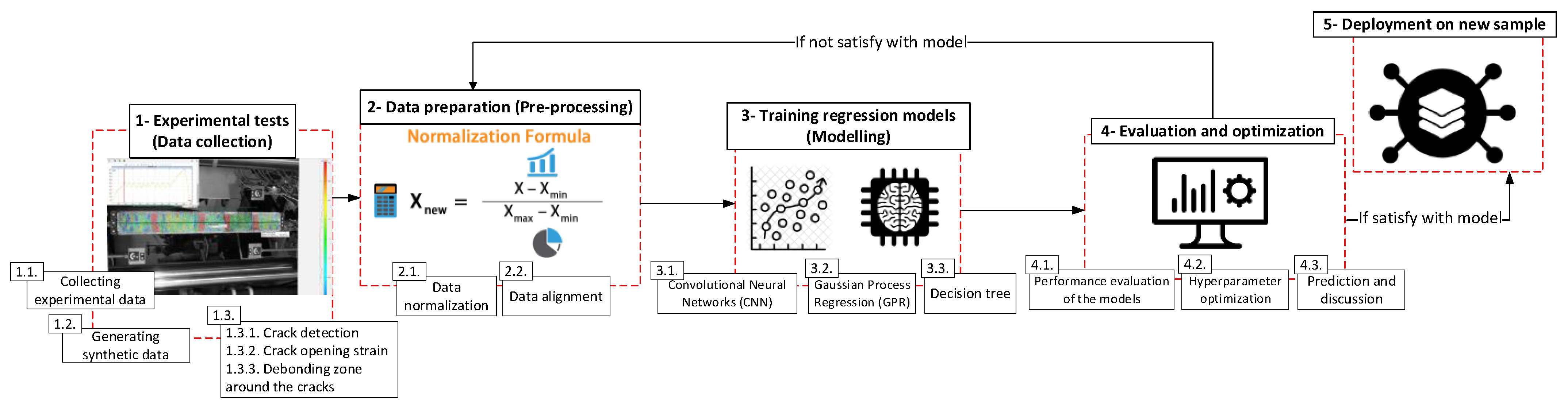
Machine learning regression is a versatile tool for uncovering complex correlations between obvious and embedded data; however, generated datasets play a key role in developing regression models. In this study, the parameters that served as the input dataset were: surface deformations monitored by DIC, the reinforcement ratio , , and as the tensile strength of concrete. The output was the response for local strain on the embedded rebar.
Four machine learning regression algorithms, including neural network (NN), Gaussian process regression (GPR), decision tree, and ensemble model, were used to generate regression models and predict strains on embedded reinforcement. Before training the models, the prepared datasets were divided into training and test groups at an 80/20 ratio to find the most efficient algorithm. It needs to be mentioned that the whole dataset collected from 2N100 was not observed in the training phase and was kept with test dataset to evaluate the performance of the model trained by the hybrid learning approach. Finally, the prepared dataset was pre-processed with data normalization along with shuffling to avoid bias towards a specific dataset.
4.2. Verification of Trained Models, Hyperparameter Optimization, and Statistical Performance Measures
Machine learning models feature several hyperparameters that can be tweaked to alter the algorithm’s performance. Thus, the accuracy of training models mainly depends on how well the hyperparameters have been tuned. However, even with the same ML model, one combination of hyperparameters is not always the best for different training datasets.
Neural networks (NN) consist of fully connected layers, including hyperparameters such as the number of layers, size of layers, and activation function. Therefore, the application of NN in data regression analysis with different preset hyperparameters approaches the lowest feasible values of the root-mean-square error (RMSE) by optimizing the model. The defined loss function was the mean square error (MSE), as in most regression models in the literature review, and the “Adam” optimizer was used for “gradient descent back-propagation” with a learning rate of 0.0001. Then, the designed models were trained for 1000 iterations.
Table 5 illustrates the RMSE values corresponding to different NN models to find the lowest obtained RMSE in both the validation and test datasets generated by the SGs andhybrid approach. For the experimental training dataset, an NN with three fully connected layers, ten nodes in each, and “tanh” as the activation function was found as the optimized model. In addition, for the hybrid training dataset, an NN with three fully connected layers with 100 nodes in each and “ReLU” as the activation function was found as the optimized model.
Searching for the best combination of hyperparameters is time-consuming and tedious. That is why, regarding the state-of-the-art technique, only NNs with two and three fully connected layers were studied to find the optimized hyperparameters. For the other three algorithms, Bayesian optimization [
16], which is a sequential design strategy for global optimization of black-box functions, was applied because it is more efficient.
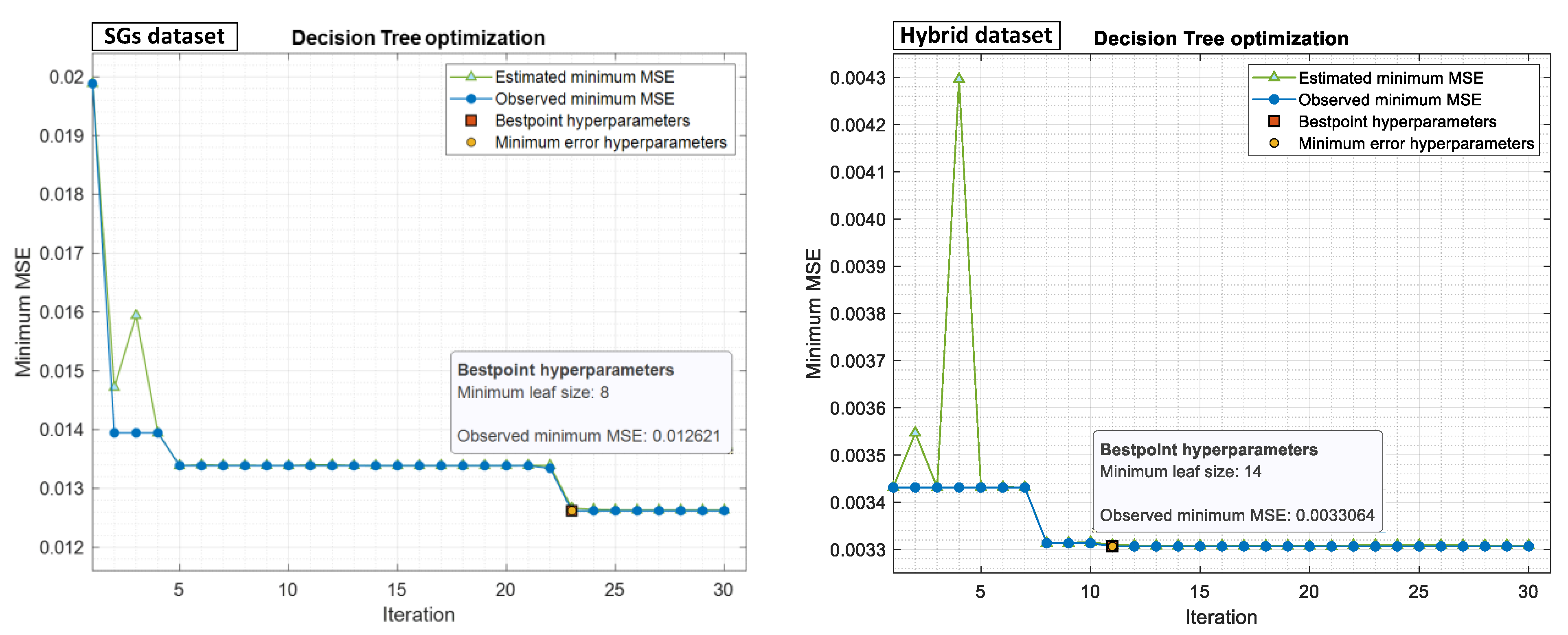
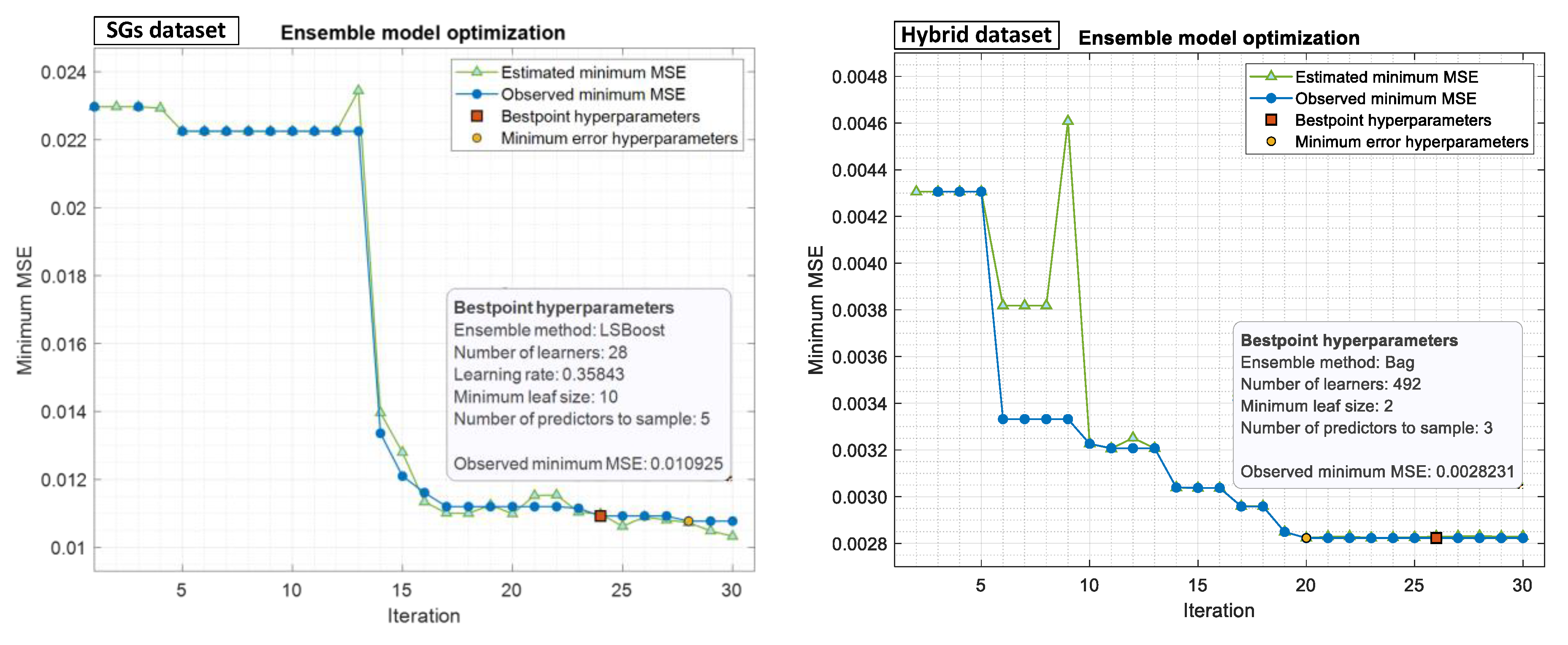
Decision Tree (DT) is a hierarchical series of binary decisions in a tree-structured model. It contains three types of nodes, including root, interior, and leaf nodes, with hyperparameters including depth of tree and minimum leaf size (also called max leaf nodes). Minimum leaf size will allow the branches of a tree to have varying depths, which is a way to control the model’s complexity. Therefore, to obtain optimized hyperparameters, the best minimum leaf size was searched using the Bayesian optimization method in the range of 1 to
, approaching minimum MSE.
Figure 13 shows the minimum leaf size obtained using the Bayesian optimization method for both prepared datasets.
It needs to be mentioned that “observed minimum MSE” means the observed minimum MSE computed so far by the optimization process. “Estimated minimum MSE” corresponds to an estimate of the minimum MSE computed by the optimization process considering all the sets of hyperparameter values tried so far and including the current iteration. In addition, “best point hyperparameters” indicates the iteration corresponding to the optimized hyperparameters, and “minimum error hyperparameters” indicates the iteration corresponding to the hyperparameters that yield the observed minimum MSE.
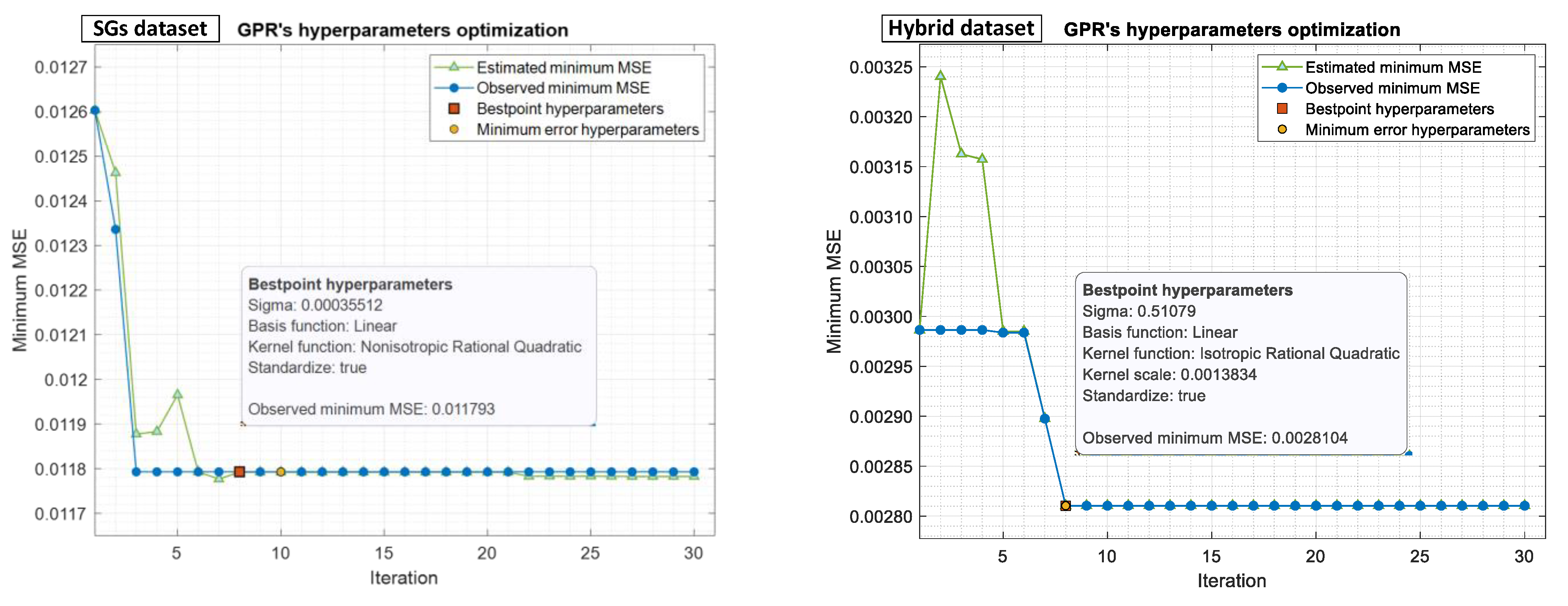
Gaussian Process Regression (GPR) is a nonparametric Bayesian approach for regression analysis that creates a significant impression in machine learning. There are several benefits to GPR, including working well on small datasets and providing uncertainty measurements on predictions. Existing hyperparameters need to be optimized, including basis function, kernel function, and scale, together with the noise standard deviation used by the algorithm, called sigma. Hyperparameter optimization was performed in 30 iterations or less, searching ranges using the Bayesian optimization method for both the SG and hybrid datasets, as shown in
Figure 14.
Sigma: 0.0001–2.1309
Basis function: Constant, Zero, Linear
Kernel function: Nonisotropic Exponential, Nonisotropic Matern 3/2, Nonisotropic Matern 5/2, Nonisotropic Rational Quadratic, Nonisotropic Squared Exponential, Isotropic Exponential, Isotropic Matern 3/2, Isotropic Matern 5/2, Isotropic Rational Quadratic, Isotropic Squared Exponential
Kernel scale: 0.001731–1.731
Ensemble model is a technique that combines multiple models and then finds the best combination to produce improved results. For this aim, bootstrap aggregation (bagging) [
17] and least-squares boosting [
18] models were used to train the regression models. Then, Bayesian optimization was used to test the different combinations of hyperparameters for both the SG and hybrid datasets to find the optimized hyperparameters in the range of 10–500 learners, with a learning rate in the range of 0.001–1 and a minimum leaf size in the range of 1 to
, as shown in
Figure 15.
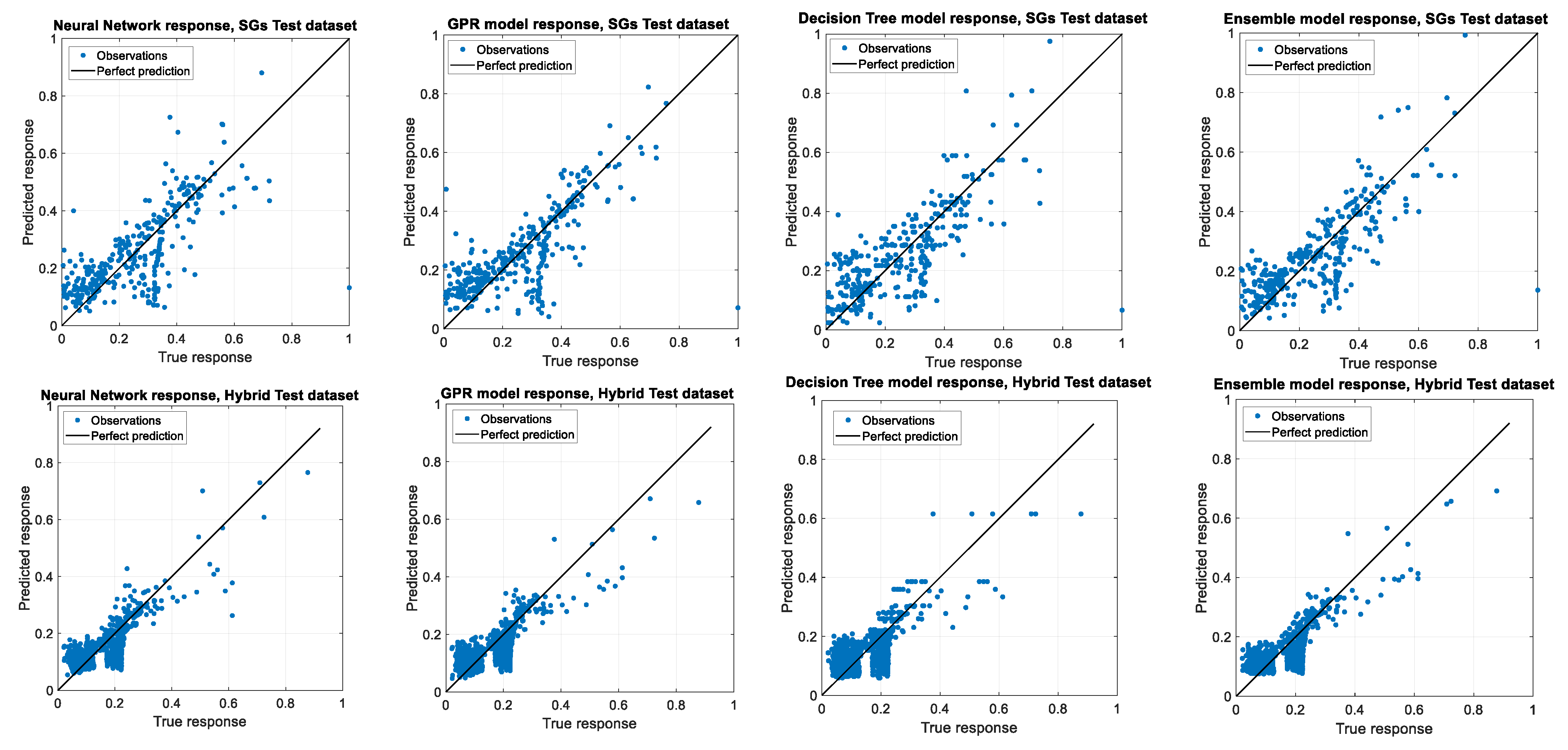
The predictions by the four optimized models compared with true values in both the experimental (SG) and hybrid datasets, according to statistical parameters.
Figure 16 shows the graphs comparing the true and predicted responses by the four optimized regression models, and
Table 6 presents the summary of the validation and accuracy tests to find the most efficient models trained by each experimental and hybrid training dataset.
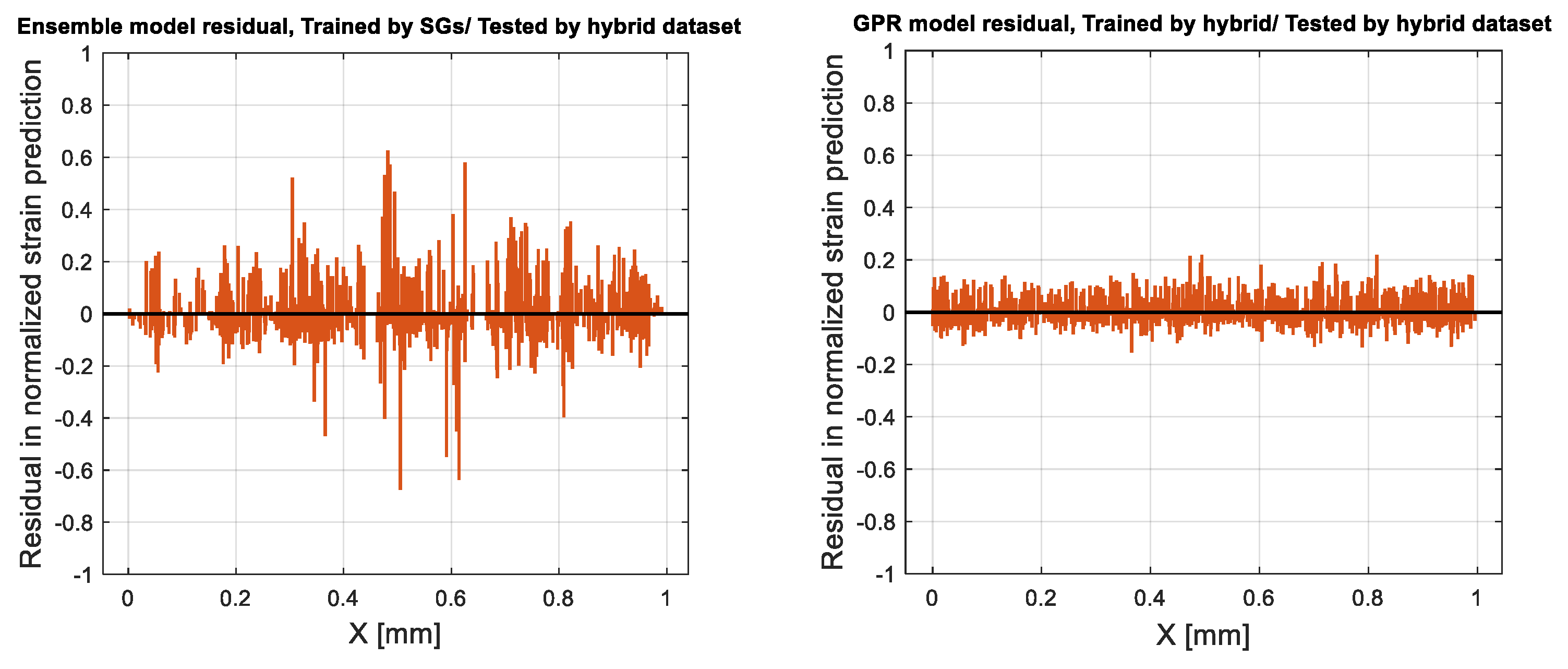
As presented in
Table 6, the ensemble model and GPR showed better performance on the training datasets generated experimentally (SG) and by the hybrid learning approach, respectively. To compare the performance of these two ML regression approaches, the residuals in normalized strain predictions are illustrated in
Figure 17. Residuals represent the difference between any data point and the regression line, which can be called “errors,” and are expressed as the difference between the predicted and observed values.
The role of concrete type and cross-sectional area in the predicted results was studied using the optimized models.
Figure 18 shows the box plots providing a visualization of residuals in normalized predictions by both optimized models for each concrete type and cross-sectional areas. The bottom and top of each box are the 25th and 75th percentiles of the predictions, respectively. The distance between the bottom and top of each box is the interquartile distribution range (IQR), which is the spread of the middle 50% of the data values. The line in the middle of each box is the prediction median; in this case it was under zero, which showed that the predictions were mostly underestimated. The whiskers are lines extending above and below each box from the end of the interquartile range to the furthest observation within the whisker length, which is equal to 1.5*IQR. Observations beyond the whisker length were marked as outliers.
Overall, the GPR model trained with a hybrid learning approach showed the best performance among all the studied models.
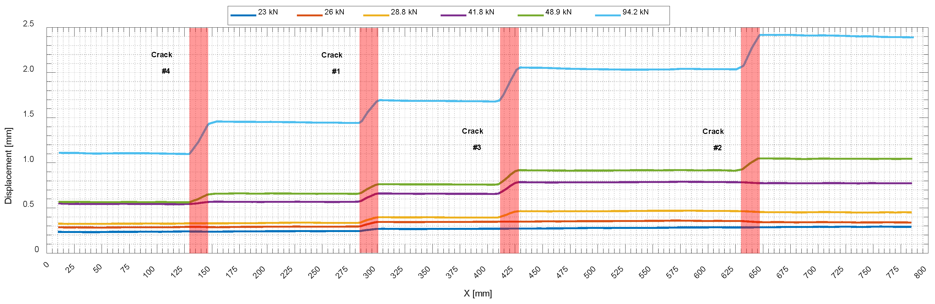
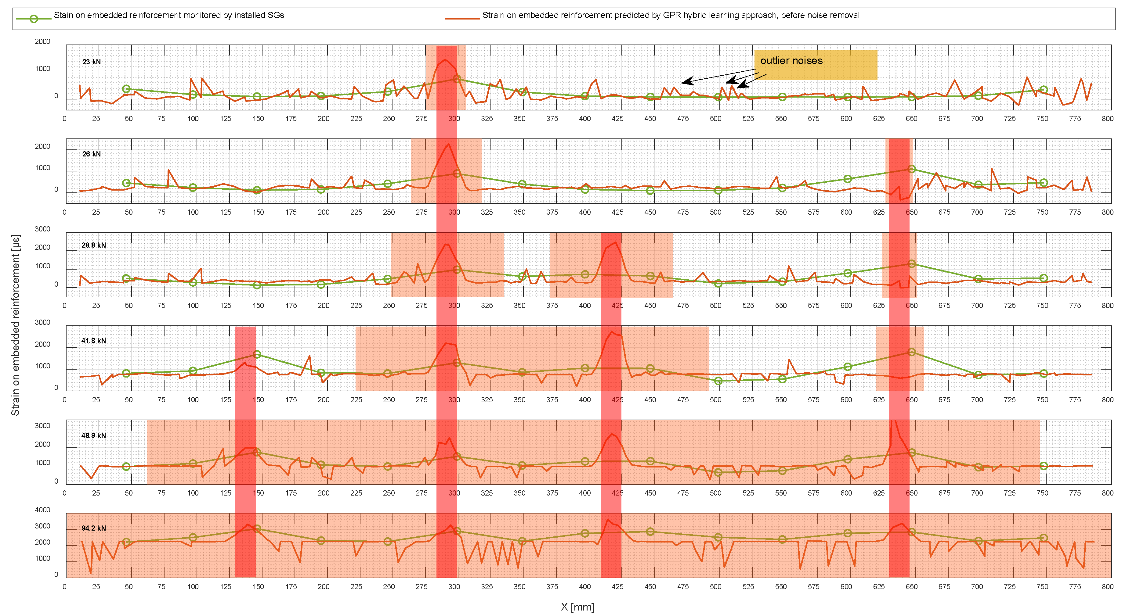
Figure 19 shows the predicted strain by the GPR model using a hybrid learning approach on embedded reinforcement for 2N100 under different loading levels. As a reminder, the obtained datasetfrom this specimen was not observed in the training phase and the predicted strain presented alongside the data collected from the installed SGs was used to verify the performance of the proposed method. There was obviously some outlier noise in the predicted values, which could be eliminated to improve the results by post-processing the predictions.
4.3. Data Improvement and Outlier Removal Using Hampel Identifier
The Hampel identifier is a statistical method used to remove outlier noise and improve the robustness of the obtained vector of prediction. The task was to perform noise removal on the predicted strain, represented by the strain as a sampled value along with the spatial location on the defined domain of the specimen. Of the total number of dataset points considered “n”, the spatial location and sampled value at the data node are given by and , respectively.
In spatial location
, in a sequence of X
1, X
2, X
3, …,
, a one-dimensional kernel with length of
is defined as a sliding window. Then, Equations (8) and (9) are used to calculate the point-to-point median
and standard deviation
in six surrounding samples, with three samples
in each side.
Therefore, outlier noise can be identified when the difference between the sampled value and local median is higher than
,
t = 3 [
19]; then, replaced with the median,
, as given by Equation (10):
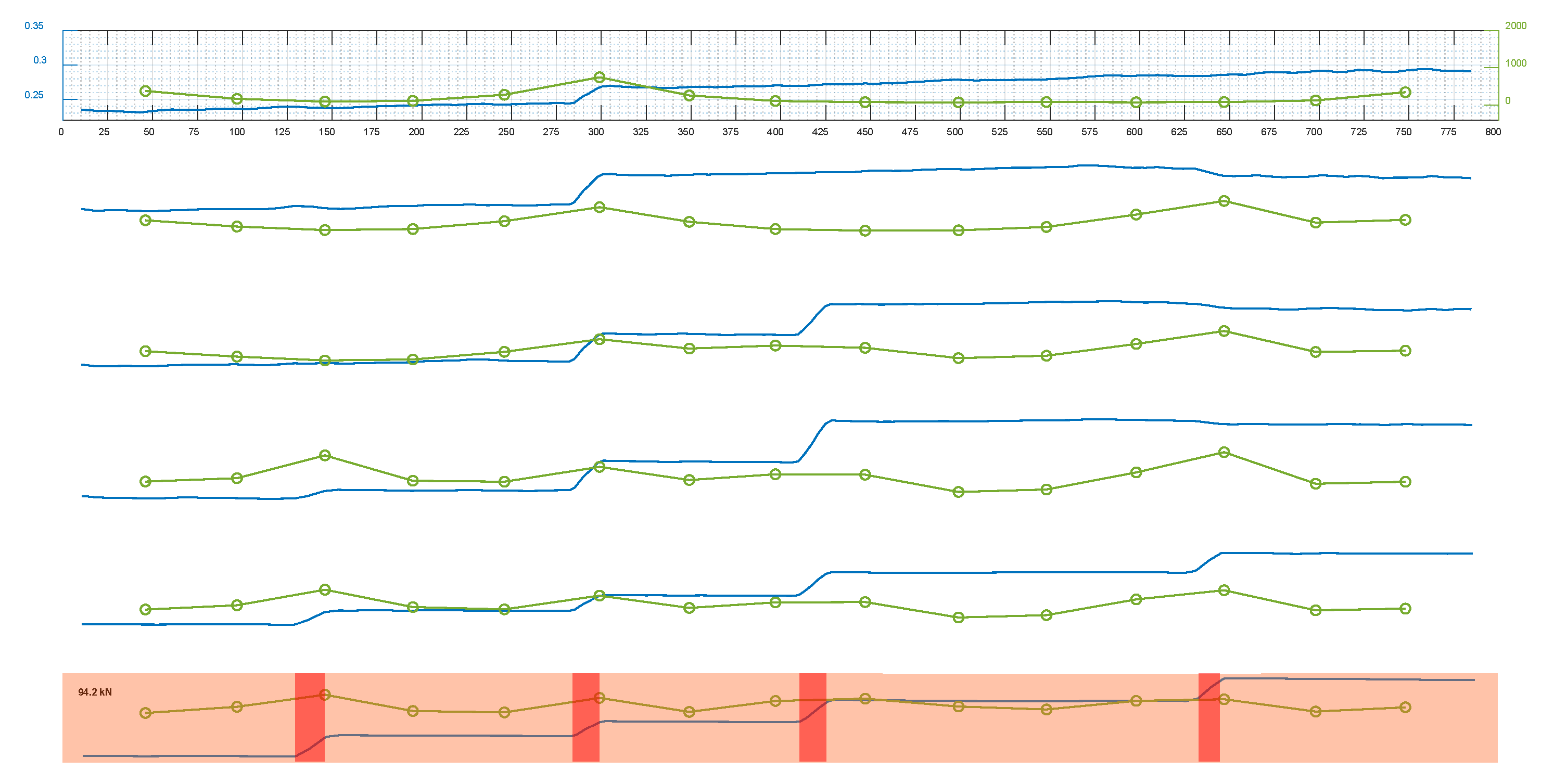
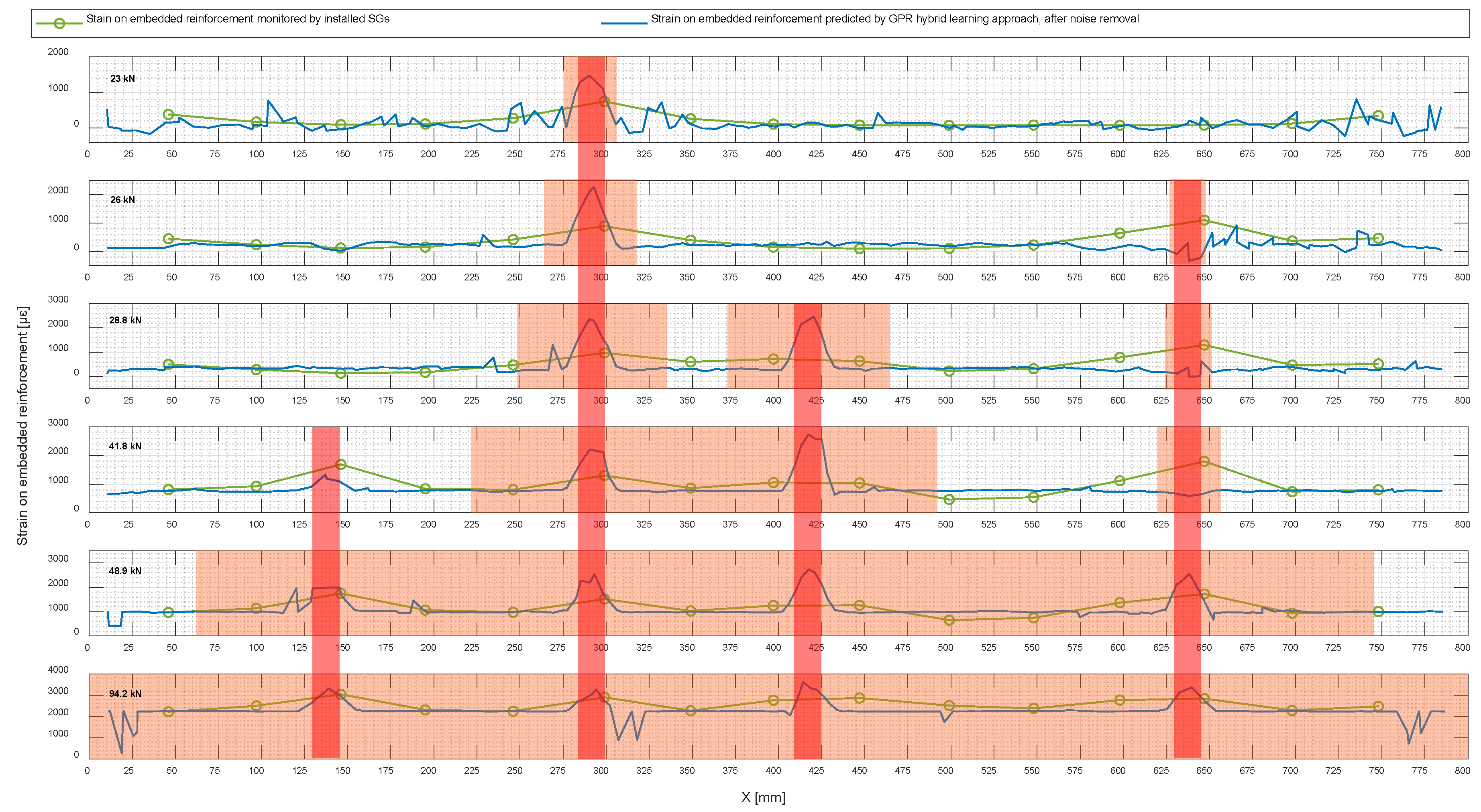
Figure 20 shows the noise-removed prediction of strain in embedded reinforcement using the hybrid learning approach alongside that obtained by monitoring the installed SGs.


