Article

Multi-Context Point Cloud Dataset and Machine Learning for Railway Semantic Segmentation

1
Unité de Recherche SPHERES, Geomatics Unit, University of Liège, 4000 Liège, Belgium
2
College of Geomatic Sciences and Surveying Engineering, Hassan II Institute of Agronomy and Veterinary Medicine, Rabat 10101, Morocco
*
Author to whom correspondence should be addressed.
Infrastructures 2024, 9(4), 71; https://doi.org/10.3390/infrastructures9040071
Submission received: 22 February 2024 / Revised: 21 March 2024 / Accepted: 28 March 2024 / Published: 9 April 2024

Abstract

:
Railway scene understanding is crucial for various applications, including autonomous trains, digital twining, and infrastructure change monitoring. However, the development of the latter is constrained by the lack of annotated datasets and limitations of existing algorithms. To address this challenge, we present Rail3D, the first comprehensive dataset for semantic segmentation in railway environments with a comparative analysis. Rail3D encompasses three distinct railway contexts from Hungary, France, and Belgium, capturing a wide range of railway assets and conditions. With over 288 million annotated points, Rail3D surpasses existing datasets in size and diversity, enabling the training of generalizable machine learning models. We conducted a generic classification with nine universal classes (Ground, Vegetation, Rail, Poles, Wires, Signals, Fence, Installation, and Building) and evaluated the performance of three state-of-the-art models: KPConv (Kernel Point Convolution), LightGBM, and Random Forest. The best performing model, a fine-tuned KPConv, achieved a mean Intersection over Union (mIoU) of 86%. While the LightGBM-based method achieved a mIoU of 71%, outperforming Random Forest. This study will benefit infrastructure experts and railway researchers by providing a comprehensive dataset and benchmarks for 3D semantic segmentation. The data and code are publicly available for France and Hungary, with continuous updates based on user feedback.

1. Introduction

Railway infrastructure plays a pivotal role in modern transportation systems, necessitating continuous innovation and precise management and maintenance [1]. The integration of advanced technologies, such as mobile LiDAR (Light Detection and Ranging), into railway applications has introduced transformative capabilities to the industry. To fully leverage these technologies, data processing methods, like semantic segmentation, are essential for understanding the complex and dynamic railway environment. Semantic segmentation, a fundamental component of computer vision, enables the categorization of each pixel in an image or point in a point cloud into predefined classes, facilitating scene understanding. In this context, machine learning has emerged as a promising approach. Deep neural networks, known for their ability to extract intricate patterns and representations from extensive datasets, offer the potential to automate critical tasks within the railway domain [2,3].
However, the effective application of machine learning in the railway environment depends on a crucial factor: the availability of annotated data. Unlike urban contexts, where several annotated datasets and benchmark are available [4,5,6,7,8], the railway environment lacks comprehensive benchmarks and annotated datasets tailored specifically to railway applications. The lack of annotated data presents a significant challenge for machine learning models development and evaluation. To train and validate semantic segmentation models effectively, labelled data, representing the diverse range of objects and structures found along railway tracks, including tracks, signals, poles, overhead wires, vegetation, and more, are required [9,10].
Moreover, as railways turn to machine learning (ML), there is a rising need for models that are accurate and easy to interpret. Using complex models, especially in safety-critical areas like railways, raises concerns about interpretation. Traditional ML models are vital for building trust, especially in tasks like semantic segmentation, in the railway environment. Additionally, the challenge extends beyond data labelling; it also involves the establishment of benchmarks that enable researchers and practitioners to objectively assess model performance. Benchmarks serve as standardized metrics for the quantitative evaluation and comparison of novel algorithms. In the absence of a railway-specific benchmark, the assessment of model performance becomes subjective and ad hoc, hindering progress and the adoption of machine learning solutions in railway applications.
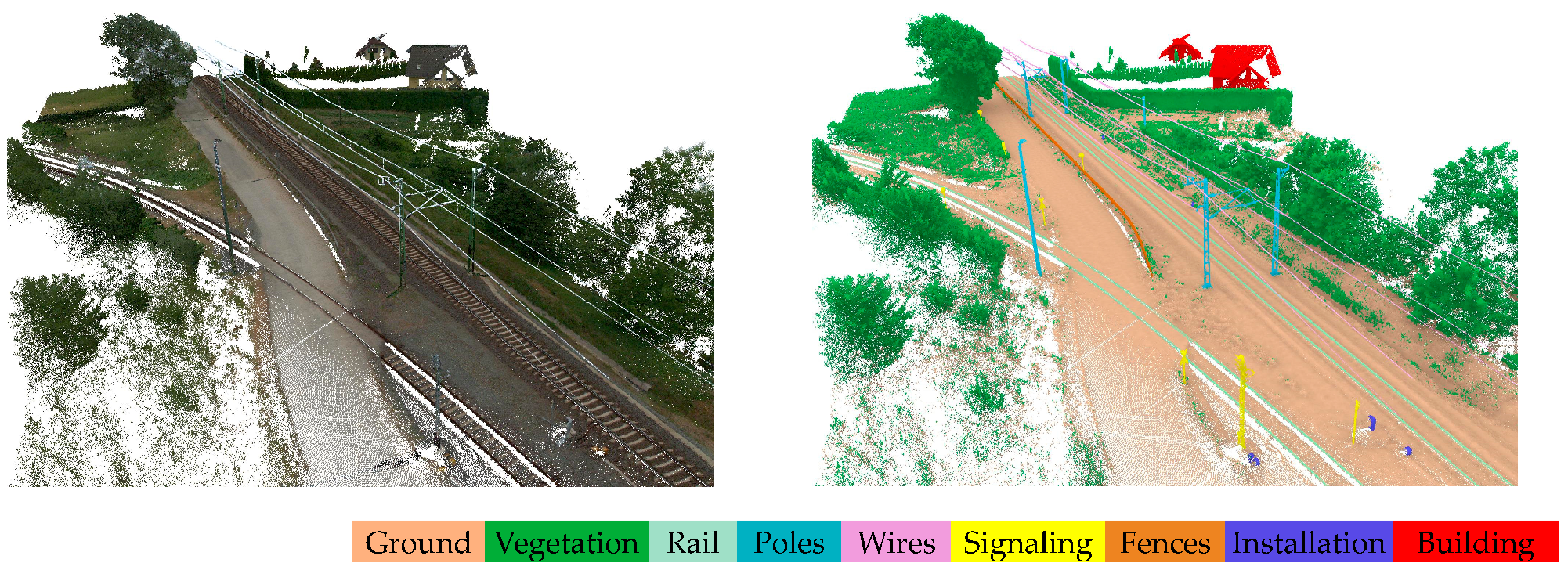
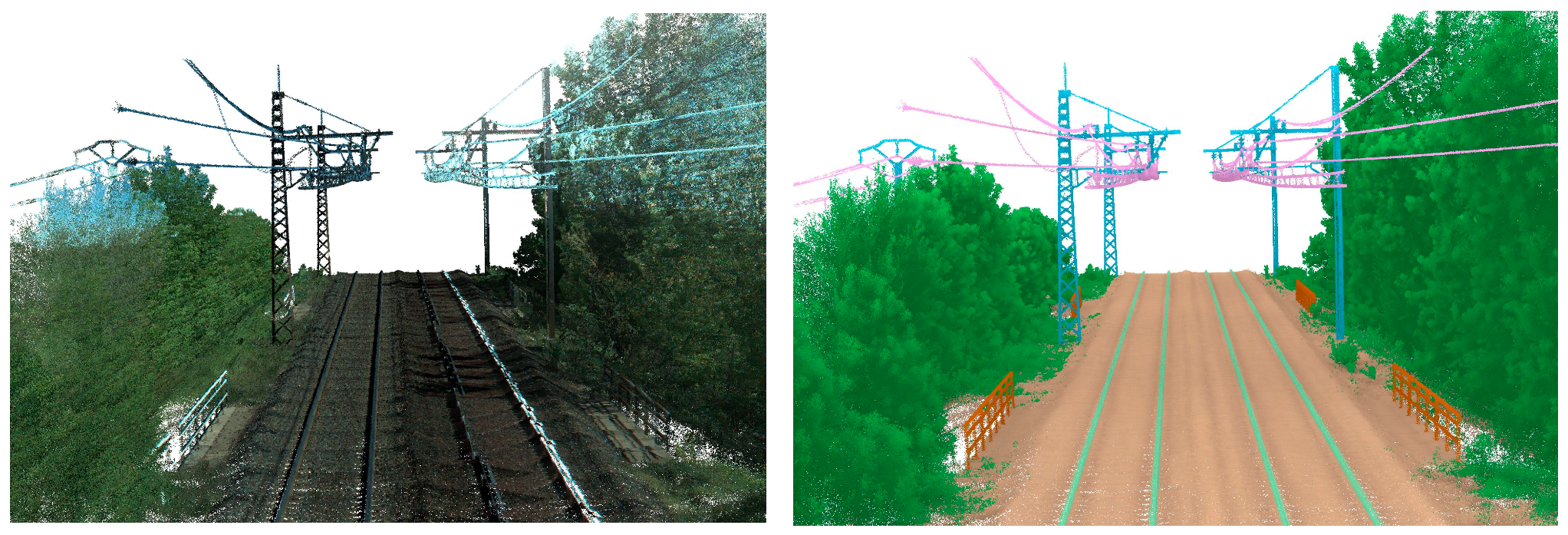
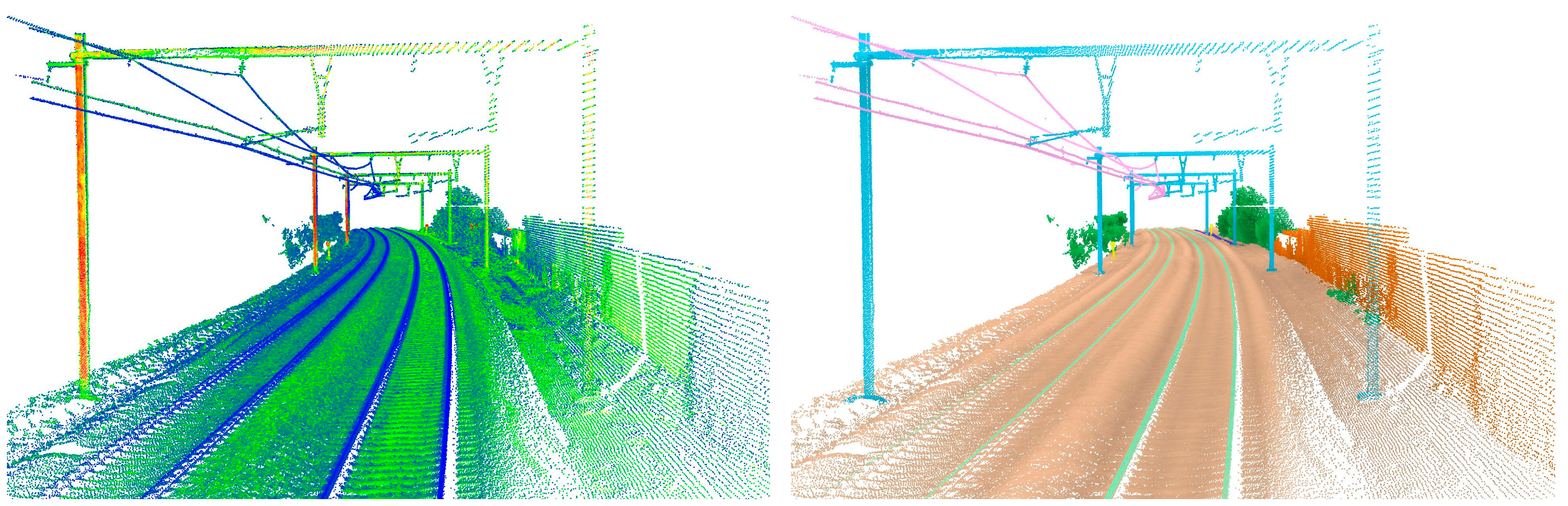
In response to this challenge, we introduce the Rail3D dataset, which aims to address the shortage of annotated data specifically tailored to railway applications. Rail3D comprises extensive point cloud data collected across diverse railway contexts in Hungary, France, and Belgium, covering approximately 5.8 km. This dataset not only mitigates the lack of annotated data but also serves as a foundational benchmark for semantic segmentation. The public availability of Rail3D represents a significant step toward fostering collaboration and innovation in the railway industry. We invite researchers, practitioners, and enthusiasts to explore, enhance, and contribute to this dataset, advancing the development of deep learning solutions that enhance the safety, efficiency, and sustainability of railway infrastructure on a global scale.
In the railway sector, where decision-makers might not be machine learning experts, the clarity and reliability of models are paramount [10]. Benchmarking LightGBM, Random Forest, and the deep-learning-based KPConv allows us to assess the effectiveness of both traditional machine learning and advanced deep learning techniques. This comparative analysis is vital for selecting a model that not only delivers high performance but is also interpretable and aligns with safety-critical standards in railway applications. Through this benchmarking process, we aim to identify a model that combines accuracy and efficiency, ensuring it can be effectively used and trusted in the context of railway infrastructure management.
The main objective of this paper is to develop a large scale and multi-context 3D point cloud dataset for railway semantic segmentation tasks and assess models’ performance on it. The contributions of our work are as follows:
  • Present a multi-context railway point cloud dataset for semantic segmentation: We introduce Rail3D, a unique dataset for railway environments. Its special because it covers a wide range of railway scenes from three countries, helping to fill the gap in available data for training machine learning models in this field.
  • Evaluate three state-of-the-art semantic segmentation models: We compare three state-of-the-art models for understanding railway scenes: KPConv, LightGBM, and Random Forest. This helps find the best tool for the task, considering what is most important in railways: accuracy and safety.
  • Assess the generalization capabilities of the best performing model: We check how well the best model works in different places. This is important to make sure the model is reliable and can be used in other real-world railway settings.
The rest of the paper is organized as follows: Section 2 presents current semantic segmentation techniques, with a special focus on railway applications and available datasets. Section 3 outlines the specifics of the subset we curated to develop Rail3D, explains how we annotated the data, and introduces the three baseline methods selected for our analysis. Section 4 details the experiments we conducted and their outcomes. Section 5 discusses what we found and ideas for future research.

2. Related Works

The availability of datasets for training has so far played a key role in the progress and comparison of ML models. These allow scene understanding across several tasks, including classification, semantic/instance/panoptic segmentation, and object detection, etc. In the following subsections, we summarize the state of the art of semantic segmentation, we investigate the existing application in railway contexts, and present the available datasets.

2.1. Semantic Segmentation

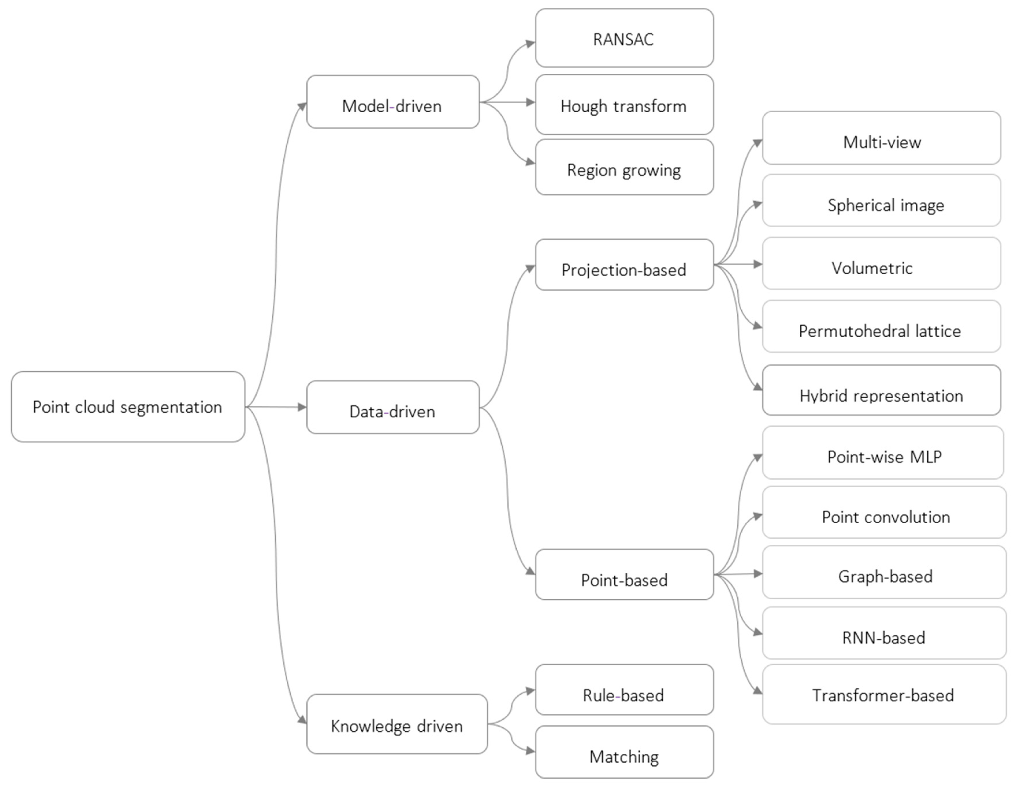
In the dynamic field of 3D point cloud semantic segmentation, significant advancements have been made through various approaches [11]. Model-driven methods, including RANSAC [12], Hough Transform, and region growing, continue to provide a solid foundation for segmenting point clouds, offering robustness in fitting geometric shapes and handling locally homogeneous properties. Meanwhile, knowledge-driven methods [13,14], incorporating explicit rules and matching strategies, are often used to enhance segmentation results in tandem with other approaches. Rule-based algorithms follow a set of predefined rules to categorize points, offering simplicity and computational efficiency [15]. Matching-based methods, on the other hand, excel in accuracy and robustness by matching the point cloud to a database of 3D models. These methods are particularly useful in scenarios where precise object recognition is essential, but they can be computationally intensive and require extensive model databases. Knowledge-driven methods often complement data-driven and model-driven approaches by refining segmentation results, ensuring that the identified objects align with domain-specific knowledge or predefined rules.
Finally, data-driven methods [11] have gained popularity, using machine and deep learning techniques to extract features and classify points. These data-driven methods span projection-based strategies, including multi-view [16,17,18,19,20,21], and spherical image approaches [22,23,24,25], as well as volumetric [26,27,28,29] and lattice-based representations [30,31,
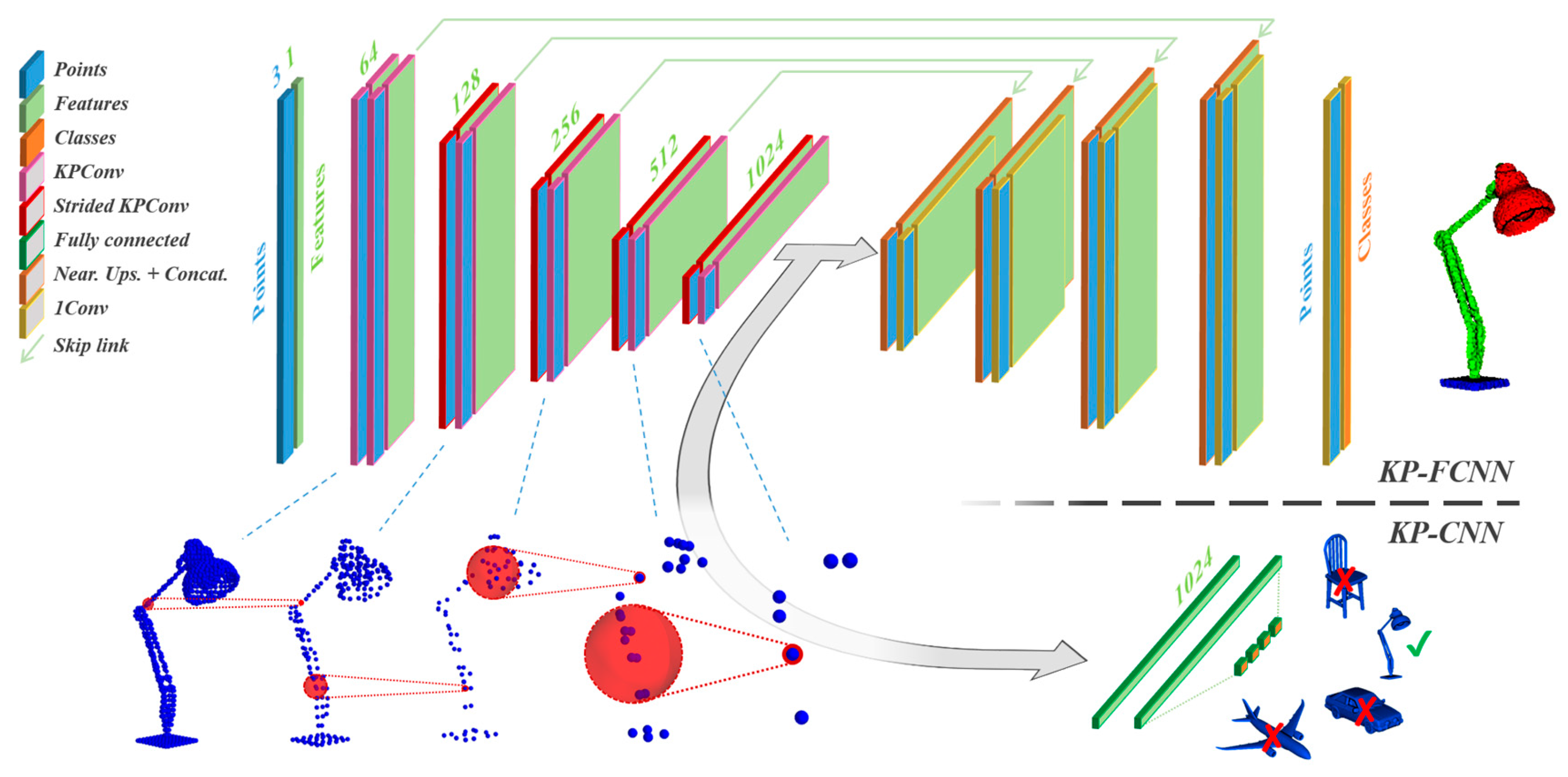
32], with hybrid representations combining their strengths. Point-based methods have made significant strides, introducing neural network architectures like PointNet and PointNet++ [33,
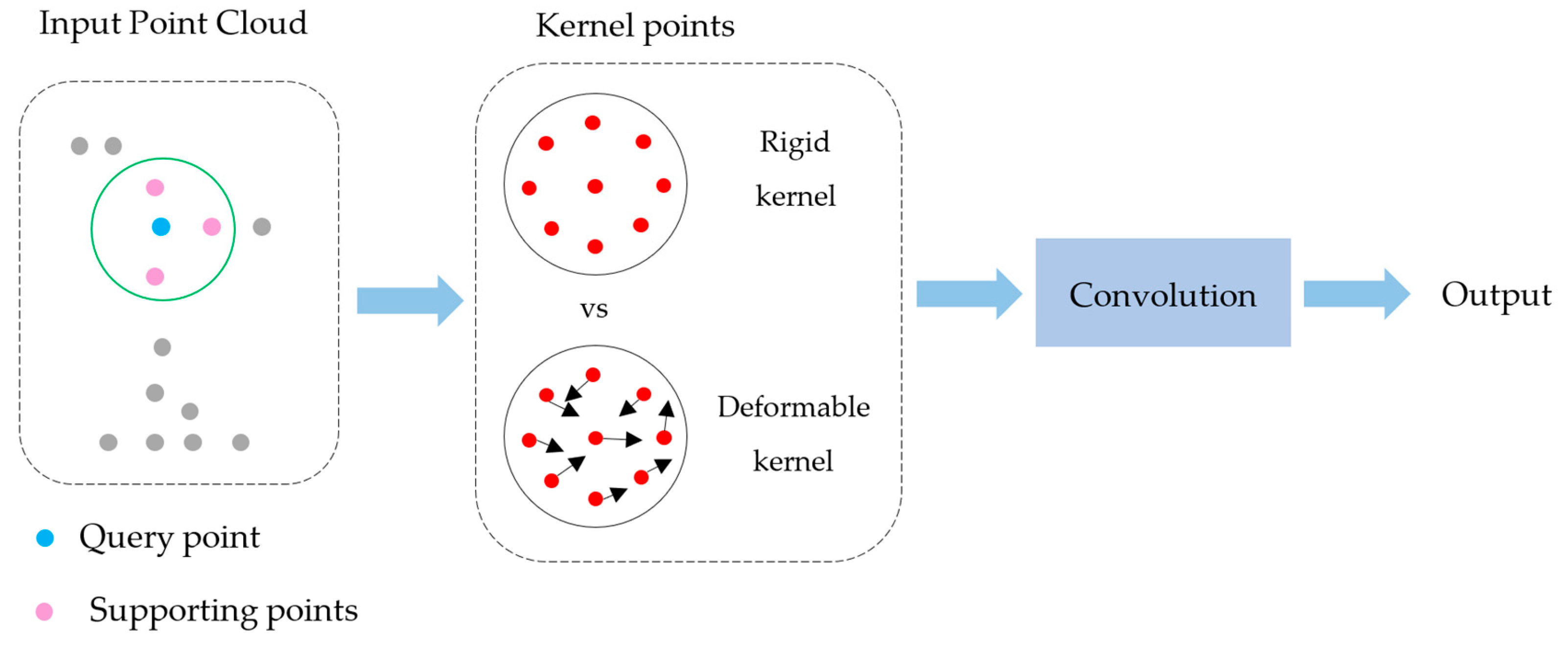
34], point convolution networks [35,36], and Graph Neural Networks [37,38,39,40] to capture complex relationships and dependencies within point clouds. Recently, transformer-based methods [41,42,43,44] have emerged as state-of-the-art, using attention mechanisms to model global dependencies in point clouds. Figure 1 summarize these semantic segmentation methods.
The most recent advances in 3D semantic segmentation include self-supervised learning, multi-task learning, transformer networks, foundation models, and 3D-LLMs. Self-supervised learning methods can train models without the need for labelled data [45]. This can be helpful for reducing the cost and effort of training 3D semantic segmentation models, especially for large-scale applications. Multi-task learning methods train models to perform multiple tasks simultaneously, such as object detection and scene understanding [46]. This can help 3D semantic segmentation models to learn better representations of the data, which can lead to improved performance on all the tasks. Transformer networks are a type of neural network architecture that has been shown to be effective for 3D semantic segmentation [41]. They can learn long-range dependencies in point clouds, which can be helpful for better results. Foundation models, such as SAM [47], are Large Visual Models (LVMs) that have been trained on a massive dataset of images and text. Foundation models can be used to train 3D semantic segmentation models in a variety of ways, such as by training a downstream model on top of the foundation model. Finally, the 3D-LLMs [48] is a new type of large language model that is specifically designed to understand and reason 3D data. 3D-LLMs can be used to perform a variety of 3D-related tasks, such as 3D captioning, 3D questions answering, and 3D-assisted dialog.

2.2. Semantic Segmentation for Railways

Even if semantic segmentation has gained progress, particularly in urban environment, applications in the railway context remain limited. Arastounia [49] developed an automated method to recognize key components of railroad infrastructure from 3D LiDAR data. The used dataset covers a 550 m section of Austrian rural railroad and contains thirty-one keys element with only XYZ coordinate information. The method segmented rail tracks, contact cables, catenary cables, return current cables, masts, and cantilevers based on their physical characteristics and spatial relationships. Recognition involved analyzing local neighborhoods, objects shape, topological relationships, and employing algorithms like KD tree’s structure [50] and FLANN’s nearest neighbor search [51] for computational efficiency. The approach achieved 96.4% accuracy and an average of 97.1% precision at point level. Despite the high metrics, this methodology cannot be generalized, the parameters need to be adjusted, and it remains particularly sensitive to occlusion. Additionally, the used data is not publicly available.
Heuristic methods have a long history, but learning-based approaches are becoming more prevalent. The latter aim to lessen reliance on parameters and enhance generalization capabilities. Chen et al. [52] proposed a method for automatically classifying railway electrification assets using mobile laser scanning data. They used a multi-scale Hierarchical Conditional Random Field (HiCRF) model to capture spatial relationships, improving classification accuracy compared to local methods. The model achieved an overall accuracy of 99.67% for ten objects classes. The authors in [53] proposed a deep learning-based methodology for the semantic segmentation of railway infrastructure from 3D point clouds. PointNet++ and KPConv were evaluated in four diverse scenarios, exhibiting a remarkable ability to adapt to varying data quality and density conditions. Notably, it achieved a mean accuracy of 90% when assessed on a 90 km long railway dataset used for both training and testing. They also evaluated the pros and cons of their approach, identifying the impact of intensity values as input features on segmentation results. Their best-performing tested architecture achieves a mean Intersection over Union (mIoU) of 74.89%. Furthermore, the methodology demonstrated its versatility by maintaining robust performance across different assets, such as rails, cables, and traffic lights, with an F1-score above 90% in all cases. Bram et al. [54] used PointNet++, SuperPoint Graph, and Point Transformer as three main deep learning models to perform semantic segmentation of railways catenary arches. The models were trained and assessed on the Railways Catenary Arches dataset with 14 labelled classes. PointNet++ achieved the best performance with over 71% in Intersection over Union (IoU).
The common disadvantage of these studies is that they do not evaluate their methods on the same dataset, in the same context, or with the same number of classes. This makes it almost impossible to make a fair comparison between all these studies, which do not, in general, make their data publicly available.

2.3. Railways Dataset

In the context of railway scene understanding, several image datasets have been developed. RailSem19 [55] offers 8500 annotated sequences from a train’s perspective, including crossings and tram scenes. FRSign (French Railway Signaling) [56] contains over one hundred thousand images annotated over six French railway traffic lights with acquisition details (time, date, sensors information, and bounding boxes). RAWPED [57,58] is dedicated to pedestrian detection in railway scenes. GERALD [59] features five thousand images and annotations for German railway signals. OSDaR23 [60], a multi-sensor dataset, captures various railway scenes with an array of sensors. These datasets are vital for developing and testing algorithms for railway scene analysis, promoting safety and automation in the industry. Compared to image datasets, there is a shortage of open 3D point cloud datasets. To date, we found the following:
  • WHU-Railway3D: Introduced by Wuhan University of Science and Technology in 2023, this is a new railway point cloud dataset. It covers 30 km, contains four billion points, and is annotated using 11 classes. Its great advantage is that it covers three different environments, including urban, rural, and plateau. Each environment covers approximately 10 km: the urban railway dataset spans 10.7 km, captured using Optech’s Lynx Mobile Mapper System in central China; the rural railway dataset, covering approximately 10.6 km, was collected through an MLS system with dual HiScan-Z LiDAR sensors; and, lastly, the plateau railway dataset, spanning around 10.4 km, was obtained using a Rail Mobile Measurement System equipped with a 32-line LiDAR sensor [61].
  • Catenary Arch Dataset: Covering an 800 m stretch of railway track near Delft, Netherlands, this dataset captures fifteen catenary arches in high detail [62]. The data collection process involved the use of a Trimble TX8 Terrestrial Laser Scanner (TLS). This dataset provides the XYZ coordinates of points but does not include color information, intensity, or normal for the points. It is referenced within the Rijksdriehoeksstelsel coordinate system using meters as units. The number of points per arch varies from 1.6 million to 11 million, and each point is manually labelled into 14 distinct classes [62].
  • OSDaR23: The Open Sensor Data for Rail 2023 dataset offers a comprehensive multi-sensor perspective of the railway environment, recorded in Hamburg, Germany during September 2021 [60,63]. It uses a railway vehicle equipped with an array of sensors, including lidar, high and low resolution RGB cameras, an InfraRed camera, and a radar. The data were acquired through a Velodyne HDL-64E lidar sensor operating at a 10 Hz frequency. These lidar data are further enriched with annotations of various object classes (20), such as trains, rail tracks, catenary poles, signs, vegetation, buildings, persons, vehicles, etc.
  • Others dataset: Several other datasets have been used for railway scene understanding tasks, but they are not publicly available or irrelevant. They include the Austrian rural railroad [49], UA_L-DoTT [64], Vigo dataset [2,53], TrainSim [65], INFRABEL-5 [66], Railway SLAM Dataset [67], MUIF [68] by the Italian Railways Network Enterprise (RFI), and MOMIT [69].
Existing 3D point cloud datasets for railway scene understanding are often restricted in size, variety, and semantic class, limiting their practical applicability. Our Rail3D dataset addresses these limitations by providing a comprehensive collection of railway environments from Hungary, France, and Belgium. This multi-context approach includes diverse railway landscapes, with various railway types, track conditions, and densities. Table 1 summarizes the datasets and their key specifications.

3. Materials and Methods

This section details the process of labelling the dataset and the methods of benchmarks. We begin by describing the data specifications and then the used classes and how the annotation process was performed. Then, we describe the three methods for semantic segmentation in railway environments.

3.1. Dataset Specification

The Rail3D dataset is the first multi-context point cloud dataset for railways semantic understanding. It is composed of three distinct datasets from Hungary, France, and Belgium, providing a diverse representation of railways. For this, we annotated three datasets named HMLS, SNCF, and INFRABEL. The firsts two datasets are publicly available, while the third one was provided by Infrabel, the Belgian railway infrastructure manager, under a confidentiality agreement. The datasets were acquired using different LiDAR sensors, ensuring a wide range of point densities and acquisition conditions. This diversity is crucial for developing robust and generalizable models for railway scene understanding. The specifications of each dataset are detailed in the subsections below.

3.1.1. Hungarian MLS Point Clouds of Railroad Environment

This LiDAR dataset represents a collection acquired by the Hungarian State Railways using the mobile mapping system (MMS)—Riegl VMX-450 high-density. These LiDAR scans were conducted from a railroad vehicle recording data at a rate of 1.1 million points per second. It exhibited high precision, with an average 3D range accuracy of 3 mm and a maximum threshold of 7 mm, ensuring high-quality data capture. The positional accuracy of the acquired point clouds averaged 3 cm, with a maximum threshold of 5 cm. This dataset not only contains georeferenced spatial information in the form of 3D coordinates but also incorporates intensity and RGB data, enhancing its utility for diverse applications. The dataset adheres to the Hungarian national spatial reference system, designated as EPSG:23700. Originally, three distinct datasets were thoughtfully selected, each representing different topographical regions within Hungary. The original data can be found in [70].

3.1.2. French MLS Point Clouds of Railroad Environment

The SNCF LiDAR dataset is a valuable resource provided by SNCF Reseau, the French state-owned railway company. This dataset comprises approximately 2 km of rail-borne LiDAR data, representing a non-annotated subset of a more extensive collection. The geospatial reference system employed for this dataset is RGF93-CC44/NGF-IGN69, ensuring its alignment with regional mapping standards and geographic referencing. The dataset is primarily presented in compressed LAZ format with a total of 16 tiles publicly available under the Open Database License (ODbL).

3.1.3. Belgian MLS Point Clouds of Railroad Environment

For several years, Infrabel, the Belgian railway infrastructure manager, was using LiDAR technology to acquire data over the country’s railways network. The lidar acquisition process involves mounting a Z + F 9012 lidar sensor on the front part of a train (EM202 vehicle) and recording the point cloud data as the train travels along the tracks. The train collects data for every railway line in Belgium at least twice a year. This is highly relevant for 3D change detection, which we will be looking at in our next studies. In addition to LiDAR, four cameras are used to capture the colors, two at the front and two at the back. However, for this application, we only used the point cloud without intensity and without colors. The point clouds were encoded in LAS format and the coordinates were in Lambert Belge 72. We chose three different areas in Belgium: Brussels, mid-way between Brussels and Ghent, and the south of Ghent. Each of these contexts presented a different challenge, either in terms of occlusion, complexity, or unbalanced classes.
As a summary, we provide, in Table 2, an overview of the Rail3D datasets, detailing key metrics such as total points, total length, attributes, and the number of tiles per set (for train, validation, and test). Overall, for each railway scene, the training data accounted 60%, the validation data accounted for about 20%, and the test data accounted for about 20%.

3.2. Classes Typology

To choose class labels, we combined literature reviews [2,53] with insights from railway industry experts from Infrabel. This approach helped us to identify classes critical for railway infrastructure applications, ensuring our labels reflect both academic and practical considerations. This resulted in the following list of classes and their corresponding objects as illustrated in Figure 2:
  • Ground (label 1): represents various ground surfaces, including rough ground, cement, and asphalt.
  • Vegetation (label 2): covers all types of vegetation present in the railway environment, such as trees and median vegetation.
  • Rail (label 3): refers to the physical track structure.
  • Poles (label 4): includes all types of poles found along the railway, such as catenary poles and utility poles.
  • Wires (label 5): covers various overhead wires, including catenary wires, power lines, and communication cables.
  • Signaling (label 6): represents all types of railways signaling equipment, such as traffic lights and traffic signs.
  • Fence (label 7): includes several types of fences and barriers used along the railways, such as security fences, noise insulation panels, and guardrails.
  • Installation (label 8): refers to larger structures that are part of the railway infrastructure, such as boxes and passenger cabins.
  • Building (label 9): covers all types of buildings located within the railway corridor, such as houses, warehouses, and stations.

3.3. Data Annotation

The quality of the annotation is a determining factor for a good dataset, as well as for all the successive tasks. As shown by Silvia et al. (2023)’s results in [71], the annotation differs from one person to another, even for the same scene and with the same class definition. This has a significant impact on the results of deep learning semantic segmentation models, with a relationship of R2 = 0.765 between the points labelled in concordance and the F1-score. Even if the discordances do not exceed 1% in general, we tried to perform an entirely manual annotation, without using any automatic algorithms. The annotation was performed on CloudCompare [72] (version 2.13.0) using the QCloudLayers tool and was controlled by a second and a third annotator. They were given guidelines to help them with the annotation process, but it was up to them to make the final decision on the class label for each point. Table 3 details points per class, revealing dominant vegetation and ground classes. The minority classes, like signals and buildings, may pose challenges for the semantic segmentation models.
In Figure 3, Figure 4 and Figure 5, we show samples of our annotation. Each color code represents a class, as indicated in the legend.

3.4. Baseline Methods

In this subsection, we explore three baseline models for semantic segmentation of our Rail3D dataset: KPConv, LightGBM, and 3DMASC. KPConv, known for its novel convolution operation tailored for point clouds, stands out for its efficiency in semantic segmentation tasks and it shows high performance over several datasets [6,8,73]. LightGBM, a gradient-boosting framework, is chosen for its accuracy and high efficiency, particularly when dealing with handcrafted features from point clouds [74]. 3DMASC, the most recent one, offers an accessible and explainable approach for point cloud classification, managing diverse datasets effectively [75]. While KPConv has shown exceptional performance in various benchmarks, LightGBM and 3DMASC are well-established in the literature, offering robust solutions for point cloud classification. Our choice of these models is based on their proven capabilities and the recent advancements they represent in the field.

3.4.1. Deep Learning Baseline

To evaluate semantic segmentation models using our datasets, we investigated the Kernel Point Convolution (KPConv) [36]. KPConv offers a novel convolution operation specifically designed for point clouds. It departs from traditional grid-based convolutions by utilizing kernel points to define local support regions. These kernel points possess learnable weights and capture the spatial relationships between points within their area of influence. Deformable KPConv further enhances this capability by adapting the location of kernel points according to the point cloud’s geometry (Figure 6). We opted for KPConv due to its ability to efficiently handle point cloud data and its demonstrated success in semantic segmentation tasks [7].
The KP-FCNN model is built as a fully convolutional network designed for point cloud semantic segmentation. Its encoder has five layers; each layer has two convolutional blocks. The first block in each layer reduces the size of the input, except for the very first layer. These blocks are like ResNet blocks but use KPConv for the convolution process, along with batch normalization and leaky ReLU activation. After the encoding process, global average pooling collects the features, which are then passed through fully connected and SoftMax layers, like how traditional image CNNs work. The decoder part of the model uses nearest neighbor upsampling to improve the detail of point-wise features, using skip connections to combine features from both the encoder and decoder at different points. The KP-FCNN architecture is detailed in the bellow illustration in Figure 7.
To handle the large size of point clouds, the model works with smaller portions of the point cloud, shaped into spheres with a set radius. This method helps manage the large amount of data effectively. Our use of the model follows the original training guidelines, including how big the input spheres are and how the kernel points are arranged. However, we simplified the input features to just a constant value (equal to 1) that represents the shape of the data points. This simplification, along with using a sphere-based method for testing and a voting system to decide the final segmentation, helps keep the segmentation accurate even with the large size and complexity of railway point clouds.

3.4.2. Machine Learning Baseline

The extraction of meaningful information from raw 3D point cloud data is crucial for the effective application of machine learning algorithms in classification tasks. We opted into the use of handcrafted features, which are carefully selected descriptors that encapsulate the geometric, spectral, and local dimensional characteristics of the point cloud. The process of feature selection and extraction is important for enhancing the capability of machine learning models to conduct accurate classifications. By selecting the right handcrafted features, the classification algorithms (Random Forest and LightGBM) can achieve a more robust understanding and interpretation of the complex railway assets. We followed the general steps:
  • Feature identification: this selection process aims to identify a set of informative attributes that effectively capture the characteristics of the points and their surrounding context. These attributes can be derived from various sources including the point cloud’s geometry, spectral information, and local dimensionality. Common geometrical features include eigenvalues of the neighborhood covariance matrix which help identify local shapes like lines, planes, contours, edge, and volume. Additionally, point density and verticality estimations can be informative for classification. In the case of lidar data, features based on multiple returns, such as the number of returns or return ratio, are valuable for distinguishing ground, buildings, and vegetation. Height variations (e.g., Z range) and radiometric information like backscattered intensity further enhance classification, especially when dealing with objects that share similar geometries.
  • Feature extraction: it involves analyzing a point’s local neighborhood to capture its geometric properties. The choice of neighborhood type, whether spherical, cylindrical, or cubic, along with the decision to compute descriptive features at single or multiple scales significantly influences the classification outcome. Multi-scale analysis has shown greater descriptive power, capturing scene elements of varying sizes and the geometric variations of objects more effectively. While optimal parameterization, including neighborhood type, number of scales, and scale radius, is crucial, automatic scale selection based on minimizing redundancy and maximizing classification accuracy is an active area of research.
  • Feature selection: high-dimensional data can harbor irrelevant or redundant features that inflate model complexity and hinder learning. Selection methods aim for an optimal feature subset, maximizing informativeness while minimizing redundancy. Filter-based methods rank features using relevance scores (e.g., Fisher’s index or information gain index) but may miss feature synergies. Wrapper and embedded methods integrate the classifier, using accuracy (wrapper) or feature importance (embedded) for selection [75].
  • Classification: this involves assigning labels to individual points within a 3D point cloud. Common approaches include instance-based methods like k-nearest neighbors (kNN) and Support Vector Machines (SVMs), as well as ensemble methods like Random Forests (RFs) and gradient-boosting algorithms like LightGBM. RFs remain popular due to their ease of use, robustness to overfitting, and ability to provide feature importance metrics. However, these individual point classifiers, including RFs, struggle to incorporate spatial context beyond what is captured in the feature vector. Contextual classification methods address this by explicitly modelling relationships between neighboring points during training. While techniques like Conditional Random Fields (CRFs) can achieve higher accuracy by leveraging spatial context, they are computationally expensive and may not perfectly capture complex relationships due to training data limitations. Our tests leverage the strengths of LightGBM, a powerful gradient-boosting algorithm, and Random Forest, while indirectly incorporating contextual knowledge through carefully chosen feature descriptors.
Our first chosen 3D point cloud classification approach relies on handcrafted features and the LightGBM Classifier, a highly efficient and accurate gradient-boosting framework. We have carefully outlined a set of steps to improve classification performance (Figure 8). Given an annotated point clouds set, we extracted features, focusing on attributes like spatial distribution and local context. We used established features based on eigenvalues, as summarized in Table 4. To manage the unordered and varying density of 3D point clouds, we utilize a multi-scale and efficient spherical neighborhood for feature computation. Then, a concatenation step of features was performed before training the classifier. Based on the features’ importance results and the performance metrics, we can even use the model directly or once it has been retrained again with only the most important features.
The eigenvalues λ 1 λ 2 λ 3 R and the corresponding eigenvectors e 1 , e 2 , e 3 R 3 of the neighborhood covariance matrix, defined by equation bellow. Where p is a given point and p ¯ is the centroid of the neighborhood N (the sphere points) [78]:
C o v   N = 1 N p N ( p p ¯ ) ( p p ¯ ) T .
The DIP feature extracted from principal components analysis (PCA) refers to the orientation or inclination of the surface at a point in the point cloud, relative to a vertical reference. Specifically, the DIP measures how much a surface “dips” away from the horizontal plane. NORMDIP (Normal Dip Angle) refines the concept of DIP by considering the angle of the surface’s inclination (or dip) relative to the normal (perpendicular) vector of the point cloud’s surface at that point. This feature requires that the point cloud has Normal calculated for each point, which represent the perpendicular direction to the surface at each point.
The use of multi-scales is essential for capturing the variability within railway scene point clouds. This method, in contrast with single-scale approaches, enhances classification performance by adapting to the diverse sizes and shapes present in the data. The selection of scales was systematically parameterized to account for object diversity and neighborhood configurations, optimizing feature extraction across different scales. For feature extraction, we utilized eigenvalues from the neighborhood covariance matrix of each point to evaluate the point cloud geometry, focusing on attributes such as linearity, planarity, sphericity, etc. (see Table 4). Feature selection was conducted using embedded strategies, notably leveraging Random Forest-based metrics to identify the most informative features (feature importance). The classification phase employed LightGBM, chosen for its gradient-boosting capabilities and efficiency in processing the selected features. The parameters for LightGBM were determined through a grid search.
The second model is 3DMASC [75], which represents an accessible and explainable method for point cloud classification. It manages several attributes, scales, and point clouds, enabling the processing of diverse point cloud datasets, including those with spectral and multiple return attributes. The feature extraction process incorporates classical 3D data multi-scale descriptors, novel spatial variation features, and dual-cloud features, ensuring a comprehensive capture of both geometrical and spectral information. Subsequent steps in scale selection and feature fusion contribute to enhanced classification performance. The method is based on Random Forest as a classification model and CloudCompare for feature extraction, selection, importance, and classification. These are calculated either based on a spherical neighborhood or the k-nearest neighbors. Table 4 showed a summary of the features we used for this test. In Random Forest classification, feature importance is determined theoretically by evaluating how each feature contributes to reducing uncertainty or impurity in the model’s predictions across all decision trees within the forest. This process involves calculating the decrease in impurity, often measured using the Gini impurity or entropy, attributed to each feature at every split point in each tree. The model aggregates these decreases across all trees to assign an importance score to each feature. The more a feature decreases impurity on average across all trees, the more important it is. This method allows us to identify which features play a crucial role in the model’s decision-making process, highlighting their relative importance in predicting the target label.

4. Experiments and Results

This section evaluates the three chosen state-of-the-art chosen methods (KPConv, LightGBM, and 3DMASC). The first subsection describes the implementation of each method to ensure replicability. The second subsection discusses the metrics used for evaluation as well as the results of the different tests performed in our study.

4.1. Implementation

These experiments required the creation of python code and the implementation of the original experiments. For 3DMASC, from feature extraction to inference, it was performed using the 3DMASC’s CloudCompare Plugin and following the training procedure in [75]. Whereas, for KPConv, we utilize PyTorch original implementation. For the training experiment we used the same procedure as in [77]. For LightGBM, we used CloudCompare Plugin for feature extraction and feature importance. Then, we created Python scripts using the LightGBM framework (version 4.3.0) for classification. The code is available at https://github.com/akharroubi/Rail3D, accessed on 14 December 2023. We adopted the training procedure in [79]. All these codes were accessed on 14 January 2024 and experiments were conducted on a workstation with a NVIDIA GeForce RTX 3090 graphics card and an i9-10980XE CPU @ 3.00 GHz with 256 GB RAM.
For the first experiment, we used KPConv without any changes to the network architecture [77]; only the hyperparameters were adapted. We used 15 kernel points with an input sphere radius of 2.5 m and a first subsampling grid size of 0.06 m to capture fine details. The convolution radius was set to 2.0 m, with a deformable convolution radius of 4.0 m for flexible feature learning. The kernel point influence was ‘linear’, and the aggregation mode was ‘sum’. We initialized the feature’s dimension at 128 and employed batch normalization with a momentum of 0.02. The model was trained for a maximum of 400 epochs, with a learning rate of 1 × 10⁻², a batch size of 5, epoch steps of 500, and a validation size of 50, optimizing for both accuracy and efficiency. In contrast to the original article, however, we did not add any input features (only X, Y, and Z coordinates), except for a constant feature equal to one, which encoded the geometry of the input points.
For the LightGBM experiment, we used the original training strategy as in [79]. When selecting a method for neighborhood extraction from point clouds, we considered cylindrical, nearest neighbor (k-NN), and spherical approaches. We chose the spherical neighborhood method. This decision was informed by research indicating that cylindrical neighborhoods can be more advantageous in extracting useful features from point clouds [78]. The spherical method was selected for its ability to uniformly capture the local structure around a point in all directions, providing a more balanced and comprehensive understanding of the point’s immediate environment. This approach ensures that the features extracted are representative of the point’s spatial context. For the parameters, we set the boosting_type to ‘gbdt’ for gradient-boosting decision tree, with num_leaves at 100 and max_depth at 30 to allow for complex model learning. The learning_rate was set to 0.05, with n_estimators at 100 for the number of boosting rounds. We also configured subsample_for_bin at 200, subsample at 0.8 for the subsample ratio of the training instance, and min_child_samples at 20 to ensure sufficient data for each tree. The class_weight was set to “balanced” to address class imbalance. We used the dataset split detailed in Table 2 for training, validation, and testing across all models, ensuring consistency in model evaluation and comparison.
For the 3DMASC experiment, we used the Random Forest method with a spherical neighborhood for feature extraction and four scales (0.5 m, 1 m, 1.5 m, and 2 m). We set the max_depth of the trees to 30 and limited the max tree count to 150, allowing the model to learn detailed features without becoming overly complex. The min sample count was set to 10, ensuring that each leaf had enough samples to make reliable decisions. The 3DMASC plugin utilizes Random Forests to inherently assign importance scores to each of the 60 features (10 features at 4 scales) employed in the analysis. To enhance the interpretability of these scores, the plugin addresses redundancy through a two-step selection process. First, a bivariate pre-selection based on information gain (IG) and Pearson’s correlation removes highly correlated features, resulting in a set with clearer importance scores. Second, the plugin implements an embedded backward selection using the RF feature importance. This process iteratively removes features with the lowest importance while monitoring the impact on model performance via Out-of-Bag (OOB) scores. The selection stops when removing a feature significantly decreases the OOB score, identified through a sliding window approach. This approach within 3DMASC combines filter-based pre-selection for interpretability with embedded selection to capture feature interactions within the RF model [75].

4.2. Evaluation

We performed both qualitative and quantitative evaluations of the semantic segmentation results. For the class-level evaluation, we used the Intersection over Union (IoU) as a metric. As a global indicator, we employed the overall accuracy (OA) and mean of the Intersection over Union (mIoU) [80]. The following equations were used to compute each of these metrics:
I o U = T P T P + F N + F P
O A = T P + T N T P + T N + F P + F N
m e a n I o U = I o U n N
where TP, TN, FP, and FN refer to true positives and negatives, false positives, and negatives, respectively. N represents the total number of classes.
According to Table 5, which shows the results on HMLS subset, LightGBM demonstrates an overall accuracy (OA) of 0.94 positioned between the 3DMASC (RF) and KPConv approaches, which achieved OAs of 0.93 and 0.97, respectively. LightGBM also achieves a mean Intersection over Union (mIoU) of 0.60, demonstrating noteworthy proficiency in precisely delineating diverse semantic classes; it displays competitive efficacy across various categories, particularly in classes like Vegetation and Wires. However, KPConv outperforms both RF and LightGBM, particularly in classes like Ground, Rail, and the minority classes.
The results on SNCF subset show that the LightGBM method demonstrates an overall accuracy (OA) of 0.93 in the semantic segmentation task, positioned between the Random Forest (RF) and KPConv approaches, which achieved OAs of 0.91 and 0.97, respectively. LightGBM also achieves a mean Intersection over Union (mIoU) of 0.67, highlighting notable performance in accurately segmenting various semantic classes. It exhibits competitive performance across various semantic classes, with notable strengths in classes such as Rail. However, KPConv outperforms both RF and LightGBM method, particularly in classes like Ground and Signaling in Table 6.
On the Infrabel subset, the LightGBM method demonstrates an overall accuracy (OA) of 0.97, confirming its position between the Random Forest (RF) and KPConv approaches, which achieved OAs of 0.96 and 0.99, respectively. LightGBM also achieves a mean Intersection over Union (mIoU) of 0.71, indicating significant performance in accurately segmenting various semantic classes. It exhibits competitive performance across a variety of semantic classes, with notable strengths in classes such as Vegetation and Wires. However, KPConv outperforms both the RF and LightGBM methods, particularly in classes like Poles and Installation in Table 7.
Feature importance analysis revealed that the Normal dip (Dip Angle) at scales of 2 m emerged as the one of the most important features, indicating their significant role in the classification accuracy. Following these, verticality at 2 m scale was also identified as key contributor to the model’s performance. These findings, visualized in our feature importance Figure 9, underscore the value of these specific features in enhancing the semantic segmentation of railway scene point clouds.
Since KPConv achieved the best performance results, we evaluated its generalization over other datasets. We conducted a series of additional experiments; we trained the model using only HMLS and assessed its performance on SNCF and INFRABEL datasets. Subsequently, we trained a larger model (KPConv**) utilizing all three datasets and evaluated its performance on the test subset. The results demonstrated a significant improvement in model generalizability when trained on a multi-context dataset. This highlights the importance of incorporating diverse data from various railway environments to develop models that can effectively handle real-world scenarios and adapt to different contexts. The results of these tests are summarized in the table below. The KPConv model trained only on HMLS gave results of 0.61 in mIoU on SNCF and 0.55 in mIoU on INFRABEL. This is mainly because the railway contexts, in general, are quite similar. But, the results were much improved when we used the whole dataset. We reached 0.76 mIoU for SNCF and 0.64 mIoU for INFRABEL. The bad result given by KPConv on the Fences class is due to its misclassification as a building even though it does not exist in INFRABEL. Also, KPConv** gave a result of almost 0 IoU in the Signaling class, as this feature was classified into the Pole class. Table 8 summarize these findings.
KPConv training was monitored by tracking both training loss and accuracy (Figure 10 and Figure 11). The training loss indicates the model’s ability to learn from the provided data, decreasing as the model fits the training examples. Conversely, accuracy reflects the model’s performance in correctly classifying points during training. A continuously decreasing loss accompanied by a rising accuracy towards a plateau suggests the model is effectively learning the semantic relationships within the point cloud data. Meanwhile, the loss ideally exhibits a continuous decrease as the model learns from the data; occasional spikes or fluctuations may occur.
In the following figure we visually show samples of the point cloud, ground truth inputs, and the results of KPConv, LightGBM, and 3DMASC, successively.
More qualitative results are presented in Appendix A for the HMLS subset, in Appendix B for the SNCF, and in Appendix C for Infrabel. Each include scenes, with the ground truth, KPConv predictions, KPConv errors, 3DMASC predictions, and 3DMASC errors. We have not visually identified any significant differences between 3DMASC and LightGBM, even though the latter gives better quantitative results. Figure 12 highlights the problem of the misclassification of a fence next to railway tracks, which was classified as a building. This problem is due to the imbalance between these two classes, given that buildings are a minority but also that this type of fence can only be found in the INFRABEL dataset. All three approaches faced the same difficulty, with KPConv being the most accurate; visually, we cannot see difference between the 3DMASC and LightGBM results.

5. Discussion

This work addresses two complementary aspects: firstly, the proposal of three subset representing different contexts of railway environments and, secondly, the introduction of three baselines to addressing semantic segmentation challenges. Regarding the proposed dataset, it presents the first comprehensive dataset for semantic segmentation in railway environments, covering three distinct railway contexts from Hungary, France, and Belgium. These datasets provide rich resources for applications in railway environments. With a significant annotation of over 288 million points, the created datasets stand out in both size and diversity compared to existing datasets. This extensive volume of annotated points enhances the dataset’s ability to cover a wide range of situations and variations within railway environments. Furthermore, the datasets developed across these railway environments ensure effective learning for machine learning models, confirming their generalization to different contexts. This was confirmed by the results obtained in Table 8.
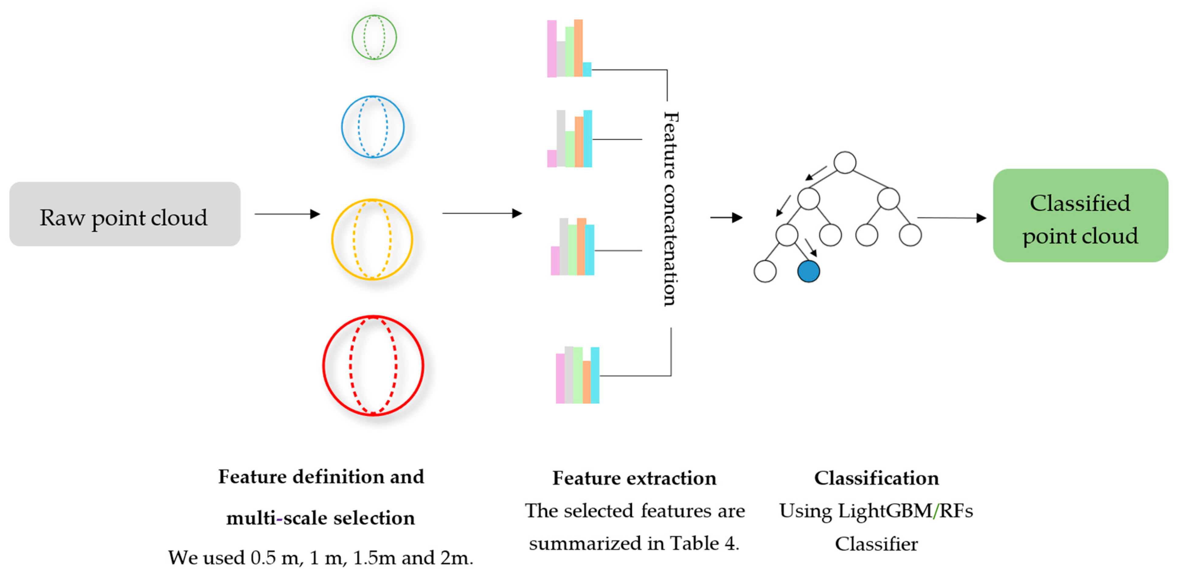
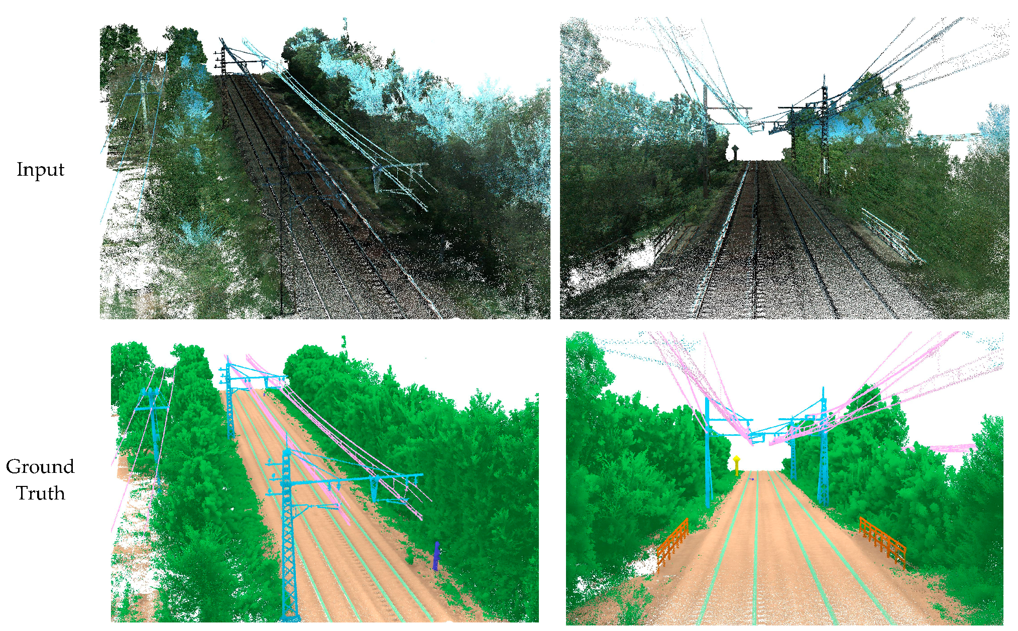
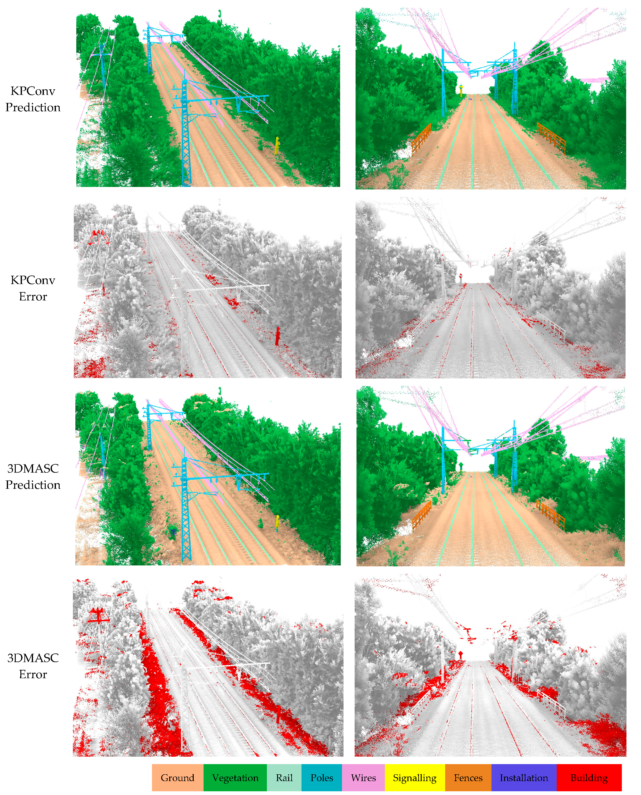
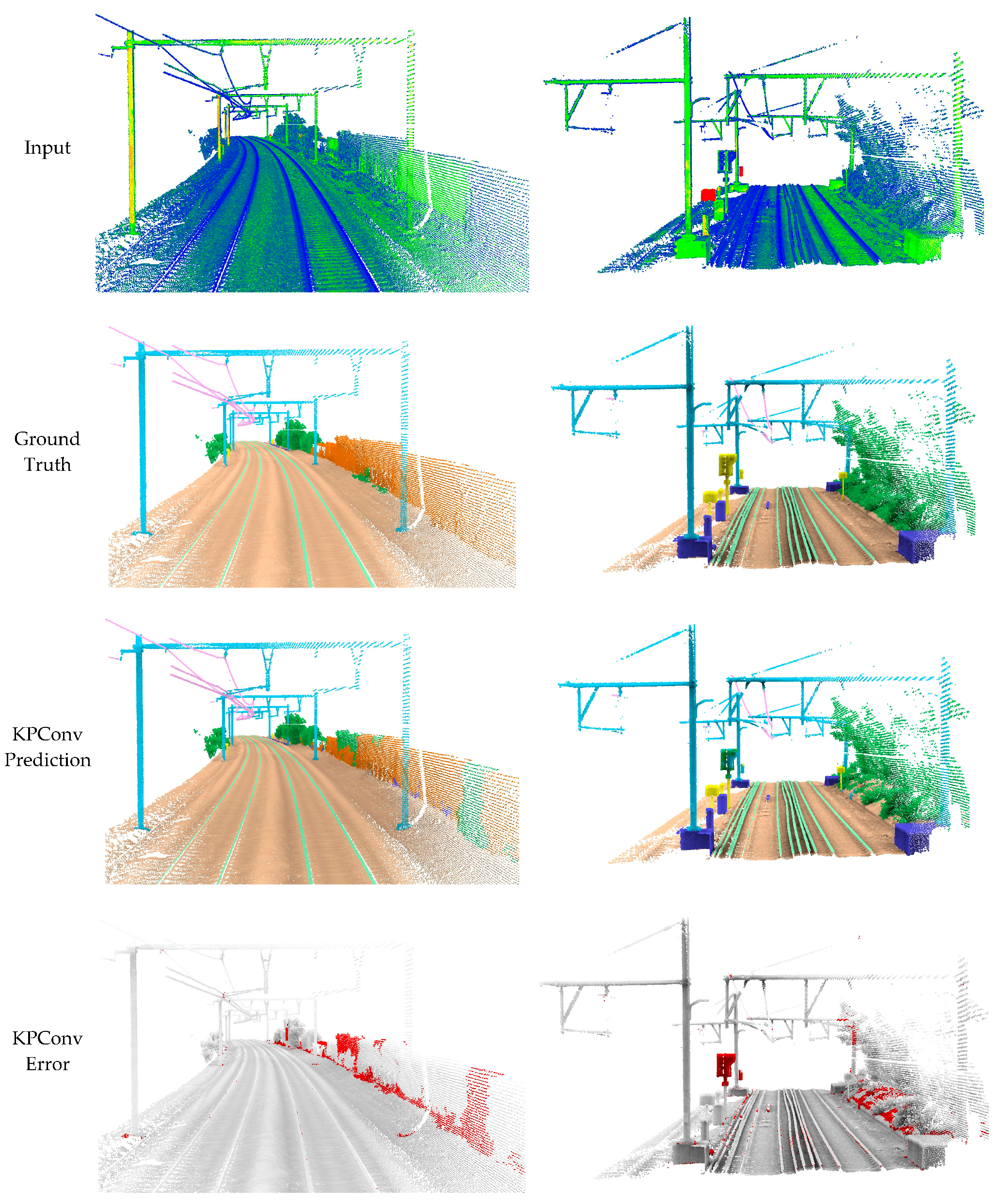
The comparison between KPConv-, 3DMASC-, and LightGBM-based results provides valuable insights about the performance of different classification methods for large-scale rail borne point cloud data. The results of the comparison indicate that, while KPConv may excel in capturing intricate local geometric features, LightGBM highlights promising performance in handling large-scale datasets with its computational efficiency. 3DMASC, although a reliable method, may exhibit limitations in dealing with the complexity and unbalanced nature of railways point cloud data. Furthermore, LightGBM offers superior computational efficiency and faster training times compared to traditional Random Forests. The performance of different methods was assessed through a combination of qualitative and quantitative evaluations. Across Table 5, Table 6 and 
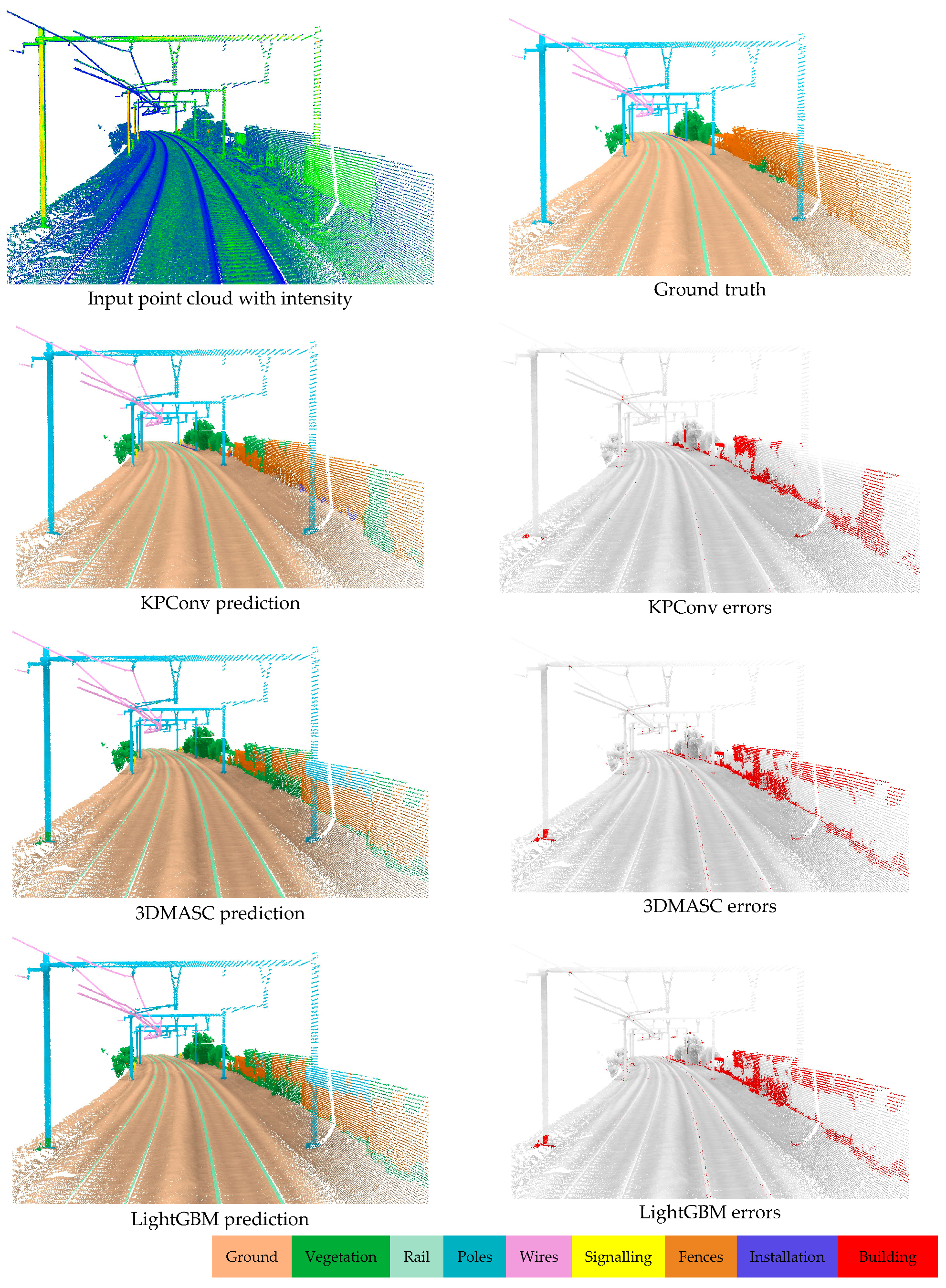
Table 7, the LightGBM method consistently gave good performance in semantic segmentation, with overall accuracies (OAs) ranging from 0.93 to 0.97 and mean Intersection over Union (mIoU) values from 0.60 to 0.71. Notably, the LightGBM approach highlights efficient results within a brief timeframe, 100 time faster than 3DMASC, emphasizing its practical applicability. This is because LightGBM is designed to be highly parallelizable while 3DMASC is not. Parallelization allows LightGBM to divide the training task into multiple smaller tasks, which can be run on multiple cores or CPUs simultaneously. While demonstrating competitive accuracy, particularly excelling in classes like Rail, Vegetation, and Wires, the machine learning method consistently falls slightly behind the performance of KPConv. The latter’s superior accuracy, especially in specific classes, suggests areas for potential refinement in the handcrafted feature method, highlighting the ongoing challenge of balancing speed and precision in semantic segmentation tasks. The qualitative results obtained using various methods have confirmed the quantitative findings. The traditional ML methods yielded qualitative results closely aligned with the ground truth across all three subsets. This underscores the good selection of geometric features, indicating a positive impact on differentiating railway objects. While color and intensity are often valuable features that can enhance classification performance, we opted to exclude them from our study for two primary reasons. Firstly, the color data acquired exhibited inferior quality due to variations in acquisition times and seasons, leading to heterogeneity between contexts. Secondly, the intensity values lacked calibration across the three contexts, as different lidar sensors were employed. To validate our choice of relying exclusively on spatial coordinates (x, y, and z) as input, we conducted a test using KPConv that verified the adverse effect of color and intensity on classification accuracy within our specific case study (refer to Figure 13). One solution to correct this sky-colored points effect would be to perform a pre-processing step, as suggested in [81].
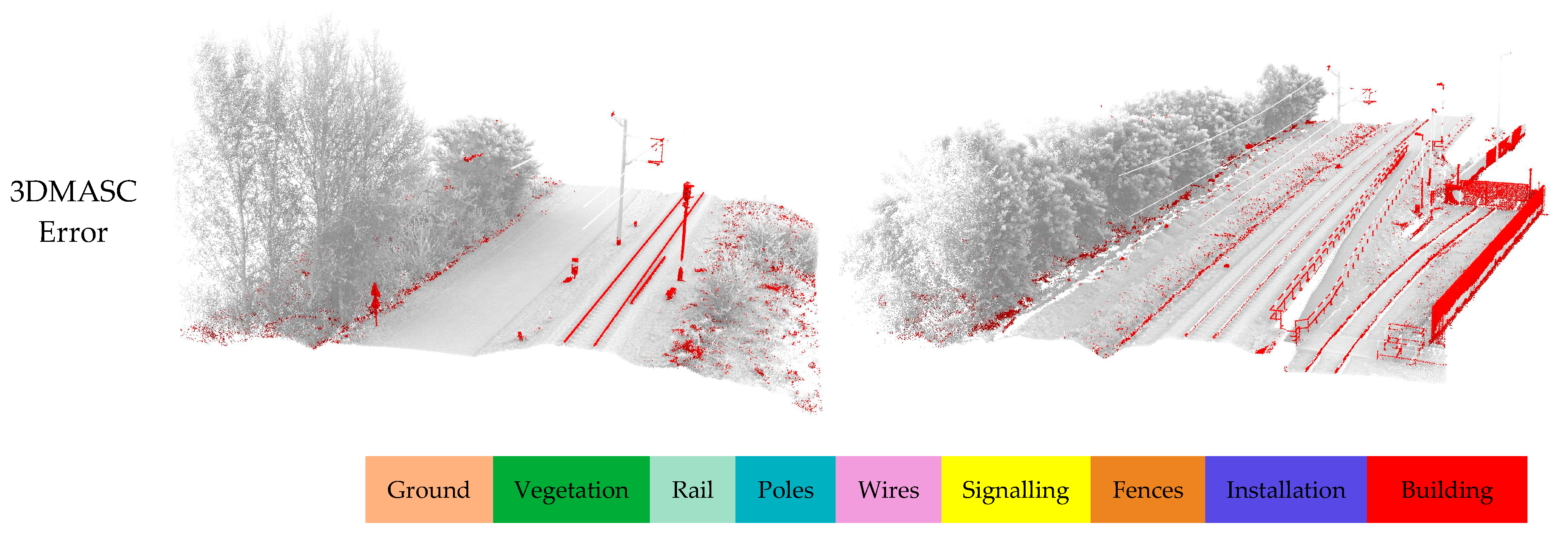
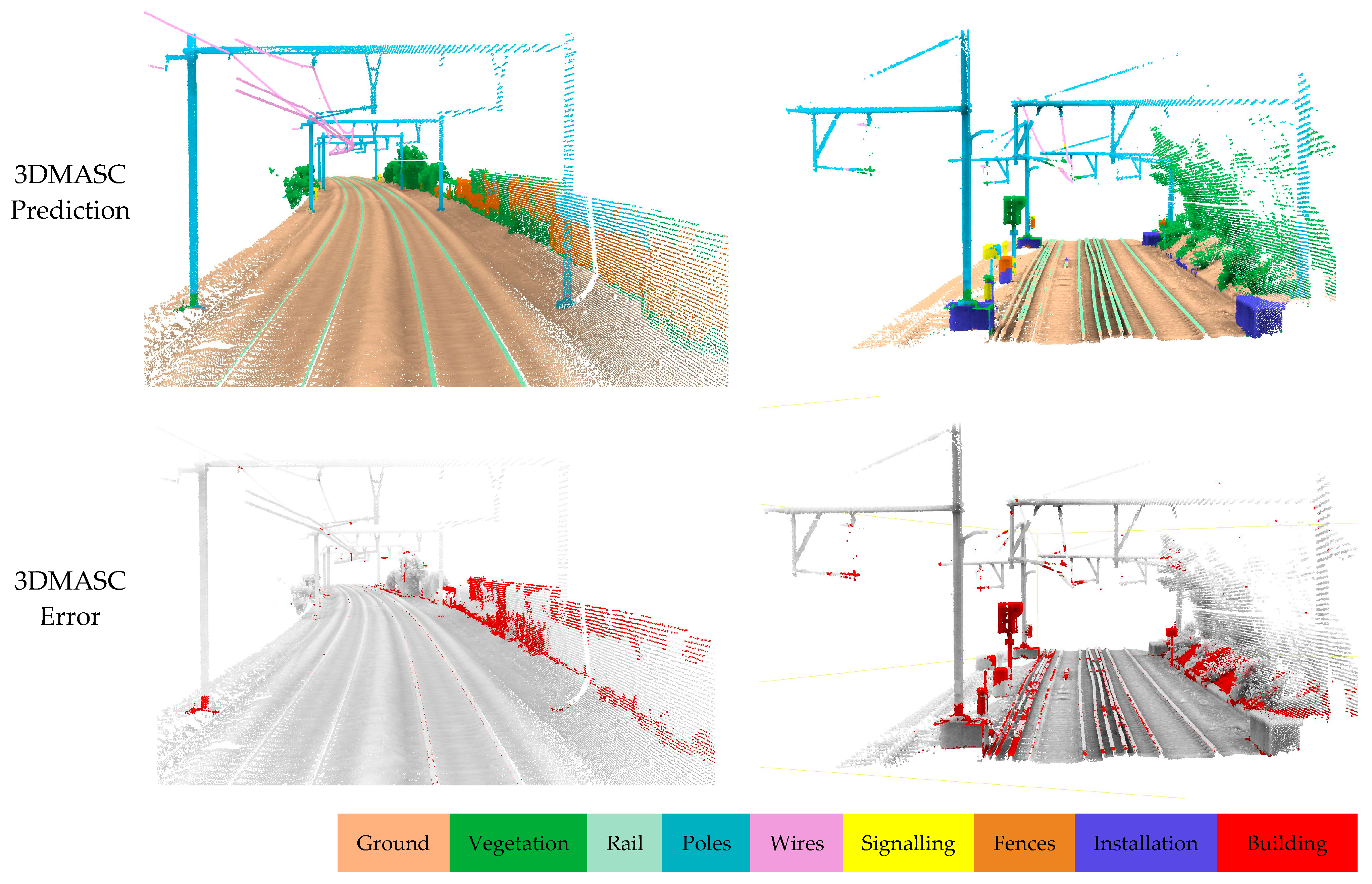
In addition, misclassification occurred where signaling poles were mistakenly categorized as catenary poles. This is due to the strong resemblance between the two and the lack of use of intensity or a specific color or geometric shape for these signs. In other cases, as shown in 
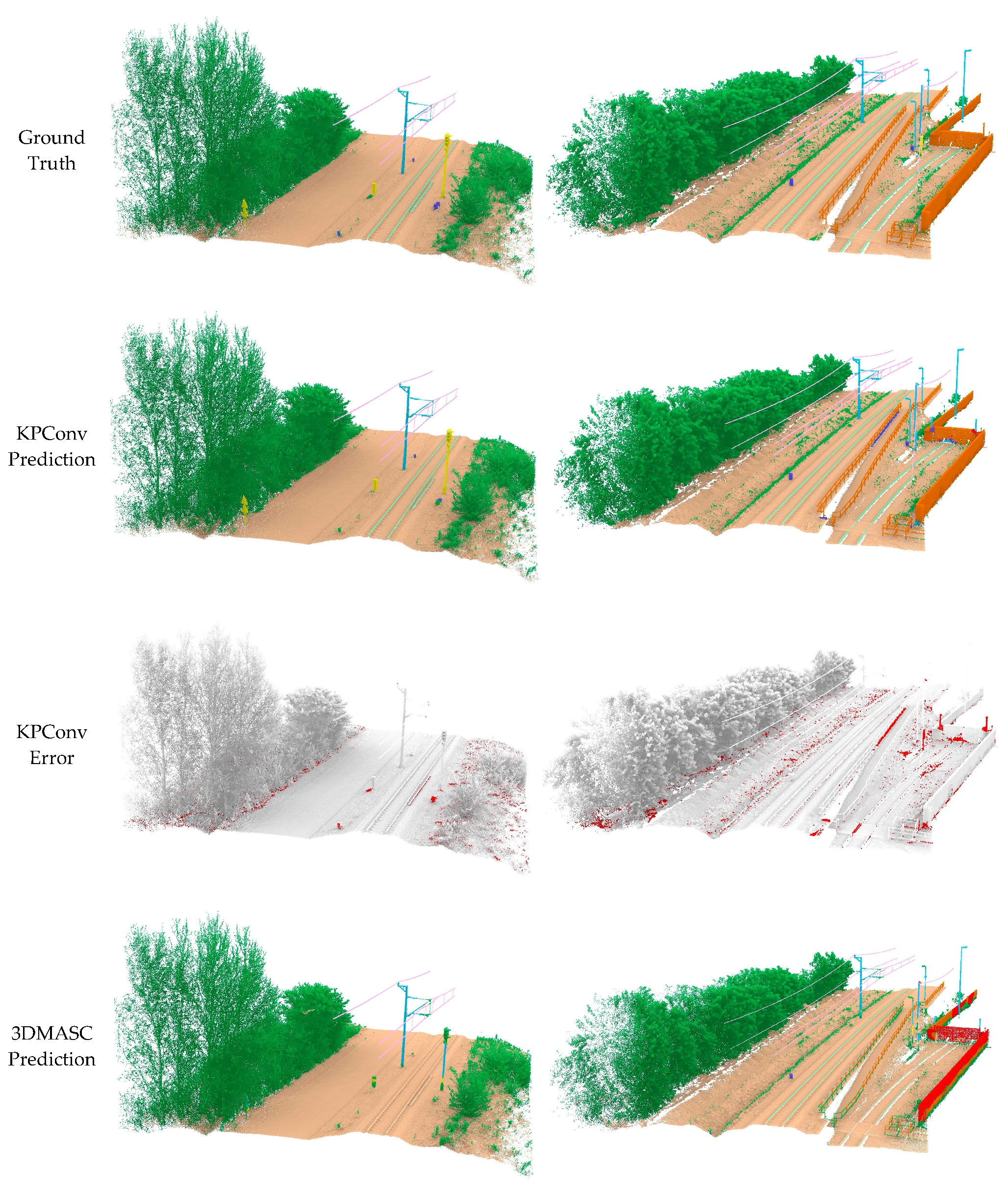
Figure 12, LightGBM and 3DMASC were unable to extract the Fence class correctly, given the strong similarity with the Building class. However, KPConv was able to classify it correctly. This led to a further experiment on KPConv to assess its generalizability. The use of a multi-context dataset, encompassing railways from three different countries, was shown to be crucial for boosting the generalizability of semantic segmentation models. By training on data from diverse railway environments, the model develops a more robust representation of railway structures and can better adapt to unseen contexts. This was demonstrated in our experiments, where the KPConv model trained on our multi-context dataset achieved significantly higher mIoU scores (0.76 and 0.64) on the SNCF and INFRABEL datasets compared to the model trained on the HMLS dataset alone (0.61 and 0.55). This suggests that our dataset can generalize to unseen railway environments, making it a valuable resource for developing robust semantic segmentation models for railway applications.

6. Conclusions

In this paper, we proposed the first multi-context point cloud dataset called Rail3D. This dataset covers three countries—Hungary, France, and Belgium—with a total length of almost 5.8 km and approximately 288 million points. It covers the nine most relevant classes for railway applications: Ground, Vegetation, Rail, Poles, Wires, Signaling, Fence, Installation, and Building. The LightGBM machine learning model for semantic segmentation demonstrated promising performance on three distinct railway datasets. It achieves significantly higher mean Intersection over Union (IoU) scores compared to 3DMASC but still falls behind the KPConv’s performance. The best performing model, a fine-tuned KPConv, achieved a mean Intersection over Union (mIoU) of 86%. Meanwhile, LightGBM achieved a mIoU of 71%, outperforming Random Forest with 70%. The Rail3D dataset, publicly available for France and Hungary at https://github.com/akharroubi/Rail3D, accessed on 14 December 2023, will overcomes limitations in existing datasets, fostering the training of more generalizable learning models. We recommend evaluating our developed dataset using new machine learning methods to assess their performance. Future work will focus on the correction of sky-colored points and experimentation on the contribution of this pre-processing step in the railway environment. It also involves the exploration of the use of semantic information within Rail3D for change detection task.

Author Contributions

Conceptualization, A.K. and R.B.; Data curation, A.K.; Funding acquisition, A.K. and R.B.; Investigation, A.K. and Z.B.; Methodology, A.K., Z.B. and R.B.; Supervision, R.B. and R.H.; Validation, R.B. and R.H.; Visualization, A.K.; Writing—original draft, A.K.; Writing—review and editing, A.K., Z.B. and A.Y. All authors have read and agreed to the published version of the manuscript.

Funding

Abderrazzaq Kharroubi is an Aspirant of the Fonds de la Recherche Scientifique FNRS.

Data Availability Statement

The data used in this study are publicly available at https://github.com/akharroubi/Rail3D (accessed on 28 November 2023).

Acknowledgments

This study is part of the first author’s Ph.D. thesis. The original data used in this study are publicly available at https://ressources.data.sncf.com/explore/dataset/nuage-points-3d for the French data and at https://data.mendeley.com/datasets/ccxpzhx9dj for the Hungarian data (accessed on 28 November 2023).

Conflicts of Interest

The authors declare no conflicts of interest.

Appendix A

Figure A1. Qualitative results on HMLS subset.
Infrastructures 09 00071 g0a1aInfrastructures 09 00071 g0a1bInfrastructures 09 00071 g0a1c

Appendix B

Figure A2. Qualitative results on SNCF subset.
Infrastructures 09 00071 g0a2aInfrastructures 09 00071 g0a2b

Appendix C

Figure A3. Qualitative results on INFRABEL subset.
Infrastructures 09 00071 g0a3aInfrastructures 09 00071 g0a3b

References

  1. Soilán, M.; Sánchez-Rodríguez, A.; Del Río-Barral, P.; Perez-Collazo, C.; Arias, P.; Riveiro, B. Review of laser scanning technologies and their applications for road and railway infrastructure monitoring. Infrastructures 2019, 4, 58. [Google Scholar] [CrossRef]
  2. Lamas, D.; Soilán, M.; Grandío, J.; Riveiro, B. Automatic point cloud semantic segmentation of complex railway environments. Remote Sens. 2021, 13, 2332. [Google Scholar] [CrossRef]
  3. Chen, X.; Chen, Z.; Liu, G.; Chen, K.; Wang, L.; Xiang, W.; Zhang, R. Railway overhead contact system point cloud classification. Sensors 2021, 21, 4961. [Google Scholar] [CrossRef]
  4. Roynard, X.; Deschaud, J.-E.; Goulette, F. Paris-Lille-3D: A Point Cloud Dataset for Urban Scene Segmentation and Classification. Available online: http://caor-mines-paristech.fr/fr/ (accessed on 14 December 2023).
  5. Tan, W.; Qin, N.; Ma, L.; Li, Y.; Du, J.; Cai, G.; Yang, K.; Li, J. Toronto-3D: A Large-scale Mobile LiDAR Dataset for Semantic Segmentation of Urban Roadways. Available online: https://www.cloudcompare.org (accessed on 14 December 2023).
  6. Behley, J.; Garbade, M.; Milioto, A.; Quenzel, J.; Behnke, S.; Stachniss, C.; Gall, J. SemanticKITTI: A Dataset for Semantic Scene Understanding of LiDAR Sequences. April 2019. Available online: http://arxiv.org/abs/1904.01416 (accessed on 14 December 2023).
  7. Lytkin, S.; Badenko, V.; Fedotov, A.; Vinogradov, K.; Chervak, A.; Milanov, Y.; Zotov, D. Saint Petersburg 3D: Creating a Large-Scale Hybrid Mobile LiDAR Point Cloud Dataset for Geospatial Applications. Remote Sens. 2023, 15, 2735. [Google Scholar] [CrossRef]
  8. Roynard, X.; Deschaud, J.-E.; Goulette, F. Paris-Lille-3D: A Large and high-quality ground truth urban point cloud dataset for automatic segmentation and classification. arXiv 2017, arXiv:1712.00032. Available online: http://arxiv.org/abs/1712.00032 (accessed on 14 December 2023). [CrossRef]
  9. Zhang, R.; Wu, Y.; Jin, W.; Meng, X. Deep-Learning-Based Point Cloud Semantic Segmentation: A Survey. Electronics 2023, 12, 3642. [Google Scholar] [CrossRef]
  10. Oh, K.; Yoo, M.; Jin, N.; Ko, J.; Seo, J.; Joo, H.; Ko, M. A Review of Deep Learning Applications for Railway Safety. Appl. Sci. 2022, 12, 572. [Google Scholar] [CrossRef]
  11. He, Y.; Yu, H.; Liu, X.; Yang, Z.; Sun, W.; Mian, A. Deep Learning Based 3D Segmentation: A Survey. arXiv 2021, arXiv:2103.05423. Available online: http://arxiv.org/abs/2103.05423 (accessed on 14 December 2023).
  12. Schnabel, R.; Wahl, R.; Klein, R. Efficient RANSAC for Point-Cloud Shape Detection. Comput. Graph. Forum 2007, 26, 214–226. [Google Scholar] [CrossRef]
  13. Truong, Q.H. Knowledge-Based 3D Point Clouds Processing. 2014. Available online: https://theses.hal.science/tel-00977434 (accessed on 14 December 2023).
  14. Ponciano, J.-J.; Roetner, M.; Reiterer, A.; Boochs, F. Object Semantic Segmentation in Point Clouds—Comparison of a Deep Learning and a Knowledge-Based Method. ISPRS Int. J. Geo-Inf. 2021, 10, 256. [Google Scholar] [CrossRef]
  15. Alkadri, M.F.; Alam, S.; Santosa, H.; Yudono, A.; Beselly, S.M. Investigating Surface Fractures and Materials Behavior of Cultural Heritage Buildings Based on the Attribute Information of Point Clouds Stored in the TLS Dataset. Remote Sens. 2022, 14, 410. [Google Scholar] [CrossRef]
  16. Su, H.; Maji, S.; Kalogerakis, E.; Learned-Miller, E. Multi-View Convolutional Neural Networks for 3D Shape Recognition. Available online: http://vis-www.cs.umass.edu/mvcnn (accessed on 14 December 2023).
  17. Hamdi, A.; Giancola, S.; Ghanem, B. MVTN: Multi-View Transformation Network for 3D Shape Recognition. Available online: https://github.com/ajhamdi/MVTN (accessed on 14 December 2023).
  18. Dai, A.; Nießner, M. 3DMV: Joint 3D-Multi-View Prediction for 3D Semantic Scene Segmentation. arXiv 2018, arXiv:1803.10409. Available online: http://arxiv.org/abs/1803.10409 (accessed on 14 December 2023).
  19. Kundu, A.; Yin, X.; Fathi, A.; Ross, D.; Brewington, B.; Funkhouser, T.; Pantofaru, C. Virtual Multi-view Fusion for 3D Semantic Segmentation. arXiv 2020, arXiv:2007.13138. Available online: http://arxiv.org/abs/2007.13138 (accessed on 14 December 2023).
  20. Boulch, A.; Guerry, J.; Le Saux, B.; Audebert, N. SnapNet: 3D point cloud semantic labeling with 2D deep segmentation networks. Comput. Graph. 2018, 71, 189–198. [Google Scholar] [CrossRef]
  21. Yang, Y.; Wu, X.; He, T.; Zhao, H.; Liu, X. SAM3D: Segment Anything in 3D Scenes. arXiv 2023, arXiv:2306.03908. Available online: http://arxiv.org/abs/2306.03908 (accessed on 14 December 2023).
  22. Wu, B.; Wan, A.; Yue, X.; Keutzer, K. SqueezeSeg: Convolutional Neural Nets with Recurrent CRF for Real-Time Road-Object Segmentation from 3D LiDAR Point Cloud. arXiv 2017, arXiv:1710.07368. Available online: http://arxiv.org/abs/1710.07368 (accessed on 14 December 2023).
  23. Wang, Y.; Shi, T.; Yun, P.; Tai, L.; Liu, M. PointSeg: Real-Time Semantic Segmentation Based on 3D LiDAR Point Cloud. arXiv 2018, arXiv:1807.06288. Available online: http://arxiv.org/abs/1807.06288 (accessed on 14 December 2023).
  24. Karara, G.; Hajji, R.; Poux, F. 3D point cloud semantic augmentation: Instance segmentation of 360° panoramas by deep learning techniques. Remote Sens. 2021, 13, 3647. [Google Scholar] [CrossRef]
  25. Ando, A.; Gidaris, S.; Bursuc, A.; Puy, G.; Boulch, A.; Marlet, R. Marlet. RangeViT: Towards Vision Transformers for 3D Semantic Segmentation in Autonomous Driving. arXiv 2023, arXiv:2301.10222. Available online: http://arxiv.org/abs/2301.10222 (accessed on 14 December 2023).
  26. Xu, Y.; Tong, X.; Stilla, U. Voxel-based representation of 3D point clouds: Methods, applications, and its potential use in the construction industry. Autom. Constr. 2021, 126, 103675. [Google Scholar] [CrossRef]
  27. Fang, Z.; Xiong, B.; Liu, F. Sparse point-voxel aggregation network for efficient point cloud semantic segmentation. IET Comput. Vis. 2022, 16, 644–654. [Google Scholar] [CrossRef]
  28. Ye, M.; Wan, R.; Xu, S.; Cao, T.; Chen, Q. DRINet++: Efficient Voxel-as-point Point Cloud Segmentation. arXiv 2021, arXiv:2111.08318. [Google Scholar]
  29. Li, H.; Guan, H.; Ma, L.; Lei, X.; Yu, Y.; Wang, H.; Delavar, M.R.; Li, J. MVPNet: A multi-scale voxel-point adaptive fusion network for point cloud semantic segmentation in urban scenes. Int. J. Appl. Earth Obs. Geoinf. 2023, 122, 103391. [Google Scholar] [CrossRef]
  30. Hang, S.; Jampani, V.; Sun, D.; Maji, S.; Kalogerakis, E.; Yang, M.-H.; Kau, J. SPLATNet: Sparse Lattice Networks for Point Cloud Processing. arXiv 2018, arXiv:1802.08275. Available online: http://arxiv.org/abs/1802.08275 (accessed on 14 December 2023).
  31. Rosu, R.A.; Schütt, P.; Quenzel, J.; Behnke, S. LatticeNet: Fast Point Cloud Segmentation Using Permutohedral Lattices. arXiv 2019, arXiv:1912.05905. Available online: http://arxiv.org/abs/1912.05905 (accessed on 14 December 2023).
  32. Rosu, R.A.; Schütt, P.; Quenzel, J.; Behnke, S. LatticeNet: Fast Spatio-Temporal Point Cloud Segmentation Using Permutohedral Lattices. arXiv 2021, arXiv:2108.03917. Available online: http://arxiv.org/abs/2108.03917 (accessed on 14 December 2023). [CrossRef]
  33. Qi, C.R.; Su, H.; Mo, K.; Guibas, L.J. PointNet: Deep Learning on Point Sets for 3D Classification and Segmentation. arXiv 2016, arXiv:1612.00593. Available online: http://arxiv.org/abs/1612.00593 (accessed on 14 December 2023).
  34. Qi, C.R.; Yi, L.; Su, H.; Guibas, L.J. PointNet++: Deep Hierarchical Feature Learning on Point Sets in a Metric Space. arXiv 2017, arXiv:1706.02413. Available online: http://arxiv.org/abs/1706.02413 (accessed on 14 December 2023).
  35. Wu, W.; Qi, Z.; Fuxin, L. PointConv: Deep Convolutional Networks on 3D Point Clouds. arXiv 2018, arXiv:1811.07246. Available online: http://arxiv.org/abs/1811.07246 (accessed on 14 December 2023).
  36. Thomas, H.; Qi, C.R.; Deschaud, J.-E.; Marcotegui, B.; Goulette, F.; Guibas, L.J. KPConv: Flexible and Deformable Convolution for Point Clouds. arXiv 2019, arXiv:1904.08889. [Google Scholar]
  37. Zeng, Z.; Xu, Y.; Xie, Z.; Wan, J.; Wu, W.; Dai, W. RG-GCN: A Random Graph Based on Graph Convolution Network for Point Cloud Semantic Segmentation. Remote Sens. 2022, 14, 4055. [Google Scholar] [CrossRef]
  38. Jiang, T.; Sun, J.; Liu, S.; Zhang, X.; Wu, Q.; Wang, Y. Hierarchical semantic segmentation of urban scene point clouds via group proposal and graph attention network. Int. J. Appl. Earth Obs. Geoinf. 2021, 105, 102626. [Google Scholar] [CrossRef]
  39. Landrieu, L.; Simonovsky, M. Large-scale Point Cloud Semantic Segmentation with Superpoint Graphs. arXiv 2017, arXiv:1711.09869. Available online: http://arxiv.org/abs/1711.09869 (accessed on 14 December 2023).
  40. Li, G.; Müller, M.; Thabet, A.; Ghanem, B. DeepGCNs: Can GCNs Go as Deep as CNNs? arXiv 2019, arXiv:1904.03751. Available online: http://arxiv.org/abs/1904.03751 (accessed on 14 December 2023).
  41. Lu, D.; Xie, Q.; Wei, M.; Gao, K.; Xu, L.; Li, J. Transformers in 3D Point Clouds: A Survey. arXiv 2022, arXiv:2205.07417. Available online: http://arxiv.org/abs/2205.07417 (accessed on 14 December 2023).
  42. Zhao, H.; Jiang, L.; Jia, J.; Torr, P.; Koltun, V. Point Transformer. arXiv 2020, arXiv:2012.09164. Available online: http://arxiv.org/abs/2012.09164 (accessed on 14 December 2023).
  43. Lai, X.; Liu, J.; Jiang, L.; Wang, L.; Zhao, H.; Liu, S.; Qi, X.; Jia, J. Stratified Transformer for 3D Point Cloud Segmentation. arXiv 2022, arXiv:2203.14508. Available online: http://arxiv.org/abs/2203.14508 (accessed on 14 December 2023).
  44. Zhou, J.; Xiong, Y.; Chiu, C.; Liu, F.; Gong, X. SAT: Size-Aware Transformer for 3D Point Cloud Semantic Segmentation. arXiv 2023, arXiv:2301.06869. Available online: http://arxiv.org/abs/2301.06869 (accessed on 14 December 2023).
  45. Fei, B.; Yang, W.; Liu, L.; Luo, T.; Zhang, R.; Li, Y.; He, Y. Self-supervised Learning for Pre-Training 3D Point Clouds: A Survey. arXiv 2023, arXiv:2305.04691. Available online: http://arxiv.org/abs/2305.04691 (accessed on 14 December 2023).
  46. Lin, X.; Luo, H.; Guo, W.; Wang, C.; Li, J. A Multi-task Learning Framework for Semantic Segmentation in MLS Point Clouds. In Artificial Intelligence and Security; Lecture Notes in Computer Science (Including subseries Lecture Notes in Artificial Intelligence and Lecture Notes in Bioinformatics); Springer Science and Business Media Deutschland GmbH: Berlin/Heidelberg, Germany, 2022; pp. 382–392. [Google Scholar] [CrossRef]
  47. Kirillov, A.; Mintun, E.; Ravi, N.; Mao, H.; Rolland, C.; Gustafson, L.; Xiao, T.; Whitehead, S.; Berg, A.C.; Lo, W.-Y.; et al. Segment Anything. arXiv 2023, arXiv:2304.02643. Available online: http://arxiv.org/abs/2304.02643 (accessed on 14 December 2023).
  48. Hong, Y.; Zhen, H.; Chen, P.; Zheng, S.; Du, Y.; Chen, Z.; Gan, C. 3D-LLM: Injecting the 3D World into Large Language Models. arXiv 2023, arXiv:2307.12981. Available online: http://arxiv.org/abs/2307.12981 (accessed on 14 December 2023).
  49. Arastounia, M. Automated recognition of railroad infrastructure in rural areas from LIDAR data. Remote Sens. 2015, 7, 14916–14938. [Google Scholar] [CrossRef]
  50. Vosselman, G.; Klein, R. Visualisation and structuring of point clouds. In Airborne and Terrestrial Laser Scanning; Vosselman, M.G., Maas, H.G., Eds.; CRC Press (Taylor & Francis): Boca Raton, FL, USA, 2010; pp. 45–81. [Google Scholar]
  51. Muja, M.; Lowe, D.G. Fast Approximate Nearest Neighbors with Automatic Algorithm Configuration. In VISAPP 2009, Proceedings of the Fourth International Conference on Computer Vision Theory and Applications, Lisboa, Portugal, 5–8 February 2009; Ranchordas, A., Araújo, H., Eds.; INSTICC Press: Lisbon, Portugal, 2009; Volume 1, pp. 331–340. [Google Scholar]
  52. Chen, L.; Jung, J.; Sohn, G. Multi-Scale Hierarchical CRF for Railway Electrification Asset Classification from Mobile Laser Scanning Data. IEEE J. Sel. Top. Appl. Earth Obs. Remote Sens. 2019, 12, 3131–3148. [Google Scholar] [CrossRef]
  53. Grandio, J.; Riveiro, B.; Soilán, M.; Arias, P. Point cloud semantic segmentation of complex railway environments using deep learning. Autom. Constr. 2022, 141, 104425. [Google Scholar] [CrossRef]
  54. Ton, B.; Ahmed, F.; Linssen, J. Semantic Segmentation of Terrestrial Laser Scans of Railway Catenary Arches: A Use Case Perspective. Sensors 2023, 23, 222. [Google Scholar] [CrossRef]
  55. Zendel, O.; Murschitz, M.; Zeilinger, M.; Steininger, D.; Abbasi, S.; Beleznai, C. RailSem19: A Dataset for Semantic Rail Scene Understanding. Available online: www.wilddash.cc (accessed on 14 December 2023).
  56. Harb, J.; Rébéna, N.; Chosidow, R.; Roblin, G.; Potarusov, R.; Hajri, H. FRSign: A Large-Scale Traffic Light Dataset for Autonomous Trains. arXiv 2020, arXiv:2002.05665. Available online: http://arxiv.org/abs/2002.05665 (accessed on 14 December 2023).
  57. Toprak, T.; Aydın, B.; Belenlioğlu, B.; Güzeliş, C.; Selver, M.A. Railway Pedestrian Dataset (RAWPED). Zenodo 2020. Available online: https://zenodo.org/records/3741742 (accessed on 14 December 2023).
  58. Toprak, T.; Belenlioglu, B.; Aydin, B.; Guzelis, C.; Selver, M.A. Conditional Weighted Ensemble of Transferred Models for Camera Based Onboard Pedestrian Detection in Railway Driver Support Systems. IEEE Trans. Veh. Technol. 2020, 69, 5041–5054. [Google Scholar] [CrossRef]
  59. Leibner, P.; Hampel, F.; Schindler, C. GERALD: A novel dataset for the detection of German mainline railway signals. Proc. Inst. Mech. Eng. Part F J. Rail Rapid Transit. 2023, 237, 1332–1342. [Google Scholar] [CrossRef]
  60. Tagiew, R.; Klasek, P.; Tilly, R.; Köppel, M.; Denzler, P.; Neumaier, P.; Klockau, T.; Boekhoff, M.; Schwalbe, K. OSDaR23: Open Sensor Data for Rail 2023. arXiv 2023, arXiv:2305.03001. Available online: http://arxiv.org/abs/2305.03001 (accessed on 14 December 2023).
  61. WHU-Railway3D: A Diverse Dataset and Benchmark for Railway Point Cloud Semantic Segmentation. Available online: https://github.com/WHU-USI3DV/WHU-Railway3D (accessed on 13 March 2024).
  62. Ton, B. Labelled High Resolution Point Cloud Dataset of 15 Catenary Arches in The Netherlands; 4TU.ResearchData: Delft, The Netherlands, 2022. [Google Scholar] [CrossRef]
  63. Tagiew, R.; Köppel, M.; Schwalbe, K.; Denzler, P.; Neumaier, P.; Klockau, T.; Boekhoff, M.; Klasek, P.; Tilly, R. Open Sensor Data for Rail 2023. arXiv 2023, arXiv:2305.03001. [Google Scholar] [CrossRef]
  64. Eastepp, M.; Faris, L.; Ricks, K. UA_L-DoTT: University of Alabama’s large dataset of trains and trucks. Data Brief 2022, 42, 108073. [Google Scholar] [CrossRef]
  65. D’Amico, G.; Marinoni, M.; Nesti, F.; Rossolini, G.; Buttazzo, G.; Sabina, S.; Lauro, G. TrainSim: A Railway Simulation Framework for LiDAR and Camera Dataset Generation. arXiv 2023, arXiv:2302.14486. Available online: http://arxiv.org/abs/2302.14486 (accessed on 14 December 2023). [CrossRef]
  66. Fayjie, R.; Vandewalle, P. Few-shot learning on point clouds for railroad segmentation. Electron. Imaging 2023, 35, 100-1–100-5. [Google Scholar] [CrossRef]
  67. Wang, Y. Railway SLAM Dataset; IEEE Dataport: Piscataway, NJ, USA, 2022. [Google Scholar] [CrossRef]
  68. Corongiu, M.; Masiero, A.; Tucci, G. Classification of railway assets in mobile mapping point clouds. In International Archives of the Photogrammetry, Remote Sensing and Spatial Information Sciences—ISPRS Archives; International Society for Photogrammetry and Remote Sensing: Hanover, Germany, 2020; pp. 219–225. [Google Scholar] [CrossRef]
  69. Riquelme, J.L.A.; Ruffo, M.; Tomás, R.; Riquelme, A.; Pagán, J.I.; Cano, M.; Pastor, J.L. 3D Point Cloud of a Railway Slope—MOMIT (Multi-Scale Observation and Monitoring of Railway Infrastructure Threats) EU Project—H2020-EU.3.4.8.3.—Grant Agreement ID: 777630. Zenodo 2020. Available online: https://zenodo.org/records/3777996 (accessed on 14 December 2023). [CrossRef]
  70. Cserep, M. Hungarian MLS Point Clouds of Railroad Environment and Annotated Ground Truth Data. Mendeley Data 2022. Available online: https://data.mendeley.com/datasets/ccxpzhx9dj/1 (accessed on 28 November 2023). [CrossRef]
  71. González-Collazo, S.M.; Balado, J.; González, E.; Nurunnabi, A. A discordance analysis in manual labelling of urban mobile laser scanning data used for deep learning based semantic segmentation. Expert Syst. Appl. 2023, 230, 120672. [Google Scholar] [CrossRef]
  72. Girardeau-Montaut, G. CloudCompare. 12 July 2023. Available online: https://www.cloudcompare.org/ (accessed on 14 December 2023).
  73. De Gélis, I.; Lefèvre, S.; Corpetti, T. Siamese KPConv: 3D multiple change detection from raw point clouds using deep learning. ISPRS J. Photogramm. Remote Sens. 2023, 197, 274–291. [Google Scholar] [CrossRef]
  74. Sevgen, E.; Abdikan, S. Classification of Large-Scale Mobile Laser Scanning Data in Urban Area with LightGBM. Remote Sens. 2023, 15, 3787. [Google Scholar] [CrossRef]
  75. Letard, M.; Lague, D.; Le Guennec, A.; Lefèvre, S.; Feldmann, B.; Leroy, P.; Girardeau-Montaut, D.; Corpetti, T. 3DMASC: Accessible, explainable 3D point clouds classification. Application to Bi-Spectral Topo-Bathymetric lidar data. ISPRS J. Photogramm. Remote Sens. 2024, 207, 175–197. Available online: https://hal.science/hal-04072068 (accessed on 14 December 2023). [CrossRef]
  76. Li, Y.; Fan, C.; Wang, X.; Duan, Y. SPNet: Multi-Shell Kernel Convolution for Point Cloud Semantic Segmentation. arXiv 2021, arXiv:2109.11610. Available online: http://arxiv.org/abs/2109.11610 (accessed on 14 December 2023).
  77. Thomas, H.; Qi, C.R.; Deschaud, J.-E.; Marcotegui, B.; Goulette, F.; Guibas, L.J. KPConv: Flexible and Deformable Convolution for Point Clouds. In Proceedings of the IEEE/CVF International Conference on Computer Vision (ICCV), Seoul, Republic of Korea, 24 October–2 November 2019. [Google Scholar]
  78. Thomas, H.; Deschaud, J.-E.; Marcotegui, B.; Goulette, F.; Le Gall, Y. Semantic Classification of 3D Point Clouds with Multiscale Spherical Neighborhoods. arXiv 2018, arXiv:1808.00495. Available online: http://arxiv.org/abs/1808.00495 (accessed on 14 December 2023).
  79. Ke, G.; Meng, Q.; Finley, T.; Wang, T.; Chen, W.; Ma, W.; Ye, Q.; Liu, T.-Y. LightGBM: A Highly Efficient Gradient Boosting Decision Tree. 2017. Available online: https://github.com/Microsoft/LightGBM (accessed on 14 December 2023).
  80. Grandini, M.; Bagli, E.; Visani, G. Metrics for Multi-Class Classification: An Overview. arXiv 2020, arXiv:2008.05756. Available online: http://arxiv.org/abs/2008.05756 (accessed on 14 December 2023).
  81. González, E.; Balado, J.; Arias, P.; Lorenzo, H. Realistic correction of sky-coloured points in Mobile Laser Scanning point clouds. Opt. Laser Technol. 2022, 149, 107807. [Google Scholar] [CrossRef]
Figure 1. Summary of 3D semantic segmentation methods.
Infrastructures 09 00071 g001
Figure 2. Illustration of each object class from the three datasets.
Infrastructures 09 00071 g002aInfrastructures 09 00071 g002b
Figure 3. Examples of our annotation of the Hungarian MLS dataset, displayed in colors (left) and corresponding classes (right). The legend is valid for the rest of the Figure 4 and Figure 5.
Infrastructures 09 00071 g003aInfrastructures 09 00071 g003b
Figure 4. Examples of our annotation of the SNCF dataset, displayed in colors (left) and corresponding classes (right).
Infrastructures 09 00071 g004
Figure 5. Point cloud from the INFRABEL dataset, displayed in intensity (left) and corresponding labels (right).
Infrastructures 09 00071 g005
Figure 6. KPConv defines a set of kernel points to aggregate local features and performs convolution on supporting points, which are selected from a range search around the query point. (Illustration adapted from [76]).
Infrastructures 09 00071 g006
Figure 7. Illustration of the Kernel Point Convolution network architecture [77] used as a baseline method in our study. The top illustration is for semantic segmentation; the bottom one is for the classification task.
Infrastructures 09 00071 g007
Figure 8. Multi-scale neighborhood selection, feature extraction, feature concatenation, and classification using LightGBM and Random Forest.
Infrastructures 09 00071 g008
Figure 9. Feature importance selected using the LightGBM results on the Infrabel subset.
Infrastructures 09 00071 g009
Figure 10. KPConv training loss on Rail3D Dataset (model named KPConv**).
Infrastructures 09 00071 g010
Figure 11. KPConv training accuracy on Rail3D dataset (model named KPConv**).
Infrastructures 09 00071 g011
Figure 12. Input point cloud, with KPConv, 3DMASC, and LightGBM predictions. Each is associated with an error relative to the ground truth. The same class colors are used in the previous figures.
Infrastructures 09 00071 g012
Figure 13. The poor quality of the colors led to poor classification (e.g., in vegetation). (Top): input. (Middle): predictions with colors. (Bottom): predictions without colors.
Infrastructures 09 00071 g013
Table 1. Statistics overview of the existing railways point cloud datasets.
DatasetYearAdditional FieldsPoints/SequencesClassesCountry
Catenary Arch2021Intensity55 million14Netherlands
WHU-Railway3D2023Intensity,
Number Of Returns
4 billion11China
OSDaR232023Intensity45 sequences20Germany
Rail3D2024RGB, Intensity288 million09France, Hungary, Belgium
Table 2. Description of datasets in numbers of points, length (in meter), attributes, and number of tiles per set (train, validation, and test).
DatasetTotal PointsTotal LengthAttributesTrainValidationTest
HMLS104,958,7962140 mX, Y, Z, R, G, B, Intensity1766
SNCF143,313,5881600 mX, Y, Z, R, G, B, Intensity1033
INFRABEL39,648,0062087 mX, Y, Z, Intensity1245
Table 3. The classes repartition of each subset.
DatasetGroundVegetationRailPolesWiresSignalingFencesInstallationBuilding
HMLS69,712,96132,208,4511,157,524667,108430,94974,687359,90774,272272,937
SNCF51,214,06485,506,9272,592,1311,390,7682,187,299110,467224,57687,3560
INFRABEL33,698,7961,381,5992,041,258654,7571,735,24224,92651,10060,3280
Table 4. Used handcrafted features [75], each one calculated at a multi-scale sphere diameter: 0.5 m, 1 m, 1.5 m, and 2 m.
Features CategoryAcronymDescription
Neighborhood featuresPCA1PCA: λ 1/(λ 1 + λ 2 + λ 3)
PCA2PCA: λ 2/(λ 1 + λ 2 + λ 3)
PCA3PCA: λ 3/(λ 1 + λ 2 + λ 3)
SPHERICITY(λ 3/λ 1)
LINEARITY(λ 1–λ 2)/λ 1
PLANARITY(λ 2–λ 3)/λ 1
VERTICALITY π 2 a n g l e ( e i , e z ) i ϵ ( 0,2 )
ZRANGEZmax—Zmin
ZMAXZmax—z
ZMINZ—Zmin
ANISOTROPYAnisotropy measure
DIPComputed from PCA
NORMDIPDip Angle (point cloud must have Normal)
Table 5. Quantitative experimental results on the HMLS dataset.
ApproachOAmIoUGroundVegetationRailPolesWiresSignalingFencesInstallationBuilding
KPConv0.970.860.950.910.940.930.990.960.900.130.99
3DMASC0.930.570.820.890.460.720.960.090.330.080.80
LightGBM0.940.600.830.910.480.750.970.200.300.150.85
Table 6. Quantitative experimental results on the SNCF dataset.
ApproachOAmIoUGroundVegetationRailPolesWiresSignalingFencesInstallation
KPConv0.970.810.920.960.790.960.990.670.970.23
3DMASC0.910.640.620.900.820.770.890.080.940.08
LightGBM0.930.670.680.920.860.780.880.160.850.20
Table 7. Quantitative experimental results on the INFRABEL dataset.
ApproachOAmIoUGroundVegetationRailPolesWiresSignalingFencesInstallation
KPConv0.990.840.990.840.950.970.990.400.690.89
3DMASC0.960.700.960.840.850.880.990.220.560.28
LightGBM0.970.710.970.860.870.890.980.250.630.26
Table 8. Quantitative results of KPConv trained on HMLS and tested on SNCF and INFRABEL. KPConv** was trained on all the dataset and tested on the test subset.
DatasetModelOAmIoUGroundVegetationRailPolesWiresSignalingFencesInstallation
SNCFKPConv0.950.610.880.940.610.840.890.260.810.24
KPConv**0.970.760.910.960.780.970.990.830.980.47
INFRABELKPConv0.980.550.980.760.860.750.970.2700.34
KPConv**0.990.640.990.820.940.880.9900.680.45
Disclaimer/Publisher’s Note: The statements, opinions and data contained in all publications are solely those of the individual author(s) and contributor(s) and not of MDPI and/or the editor(s). MDPI and/or the editor(s) disclaim responsibility for any injury to people or property resulting from any ideas, methods, instructions or products referred to in the content.

