Global Warming and Its Effect on Binder Performance Grading in the USA: Highlighting Sustainability Challenges

Abstract

The mounting impacts of climate change on infrastructure demand proactive adaptation strategies to ensure long-term resilience. This study investigates the effects of predicted future global warming on asphalt binder performance grade (PG) selection in the United States using a time series method. Leveraging Long-Term Pavement Performance (LTPP) data and Superpave protocol model, the research forecasts temperature changes for the period up to 2060 and calculates the corresponding PG values for different states. The results reveal significant temperature increases across the majority of states, necessitating adjustments in PG selection to accommodate changing climate conditions. The findings indicate significant increases in average 7-day maximum temperatures across the United States by 2060, with 38 out of 50 states likely to experience rising trends. Oregon, Utah, and Idaho are anticipated to face the largest temperature increases. Concurrently, the low air temperature has risen in 33 states, with notable increases in Maine, North Carolina, and Virginia. The widening gap predicted between required high and low PG poses challenges, as some necessary binders cannot be produced or substituted with other grades. The study highlights the challenge of meeting future PG requirements with available binders, emphasizing the need to consider energy consumption and CO₂ emissions when using modifiers to achieve the desired PG properties.

1. Introduction

The mounting impacts of climate change on human and natural environments are becoming more evident. Currently, the emission of greenhouse gases is causing significant changes in the Earth’s climate, leading to irreversible changes to both human well-being and the environment. These changes surpass the ability of current systems to adapt effectively [1,2]. The majority of increases in greenhouse gas emissions are caused by population growth, economic expansion, technological improvement, or changes in human behavior [3].

In 2015, human-made global greenhouse gas emissions totaled 49.1 GtCO₂eq, which was 50% higher than the emissions in 1990. Developed countries experienced a 9% decrease, while low-to-medium income countries saw a substantial 130% increase [4]. Between 1880 and 2012, emissions linked to major industrial carbon producers were responsible for 57% of the observed increase in atmospheric CO₂ levels, 42–50% of the rise in global mean surface temperature, and 26–32% of the global sea level rise [5]. Considering current trends and accounting for uncertainties related to climate change, it is estimated that the probable range of global temperature increase by the year 2100 will be between 2.0 °C and 4.9 °C. There is a 5% chance that the increase could be less than 2 °C (approximately 1.5 °C) [6].

Given the temperature sensitivity of bitumen and asphalt mixtures, as well as the typical assumption of a pavement’s lifespan (usually 20 to 30 years in the design process), it becomes crucial to consider climate change when selecting materials. Specifically, attention should be paid to choosing materials that are suitable for the climatic conditions of the region at the end of their service life. Due to the intricate properties of bitumen and the need to predict asphalt mixture behavior under varying weather conditions, traditional physical tests like penetration or softening point tests are no longer sufficient for determining the appropriate bitumen for a pavement project [7,8]. To achieve this, the Superpave protocol designed during the Strategic Highway Research Program (SHRP) project should be used to select the appropriate type of bitumen [9].

The Superpave protocol has been proposed to develop test tools and methods to standardize the use of rheological properties acquired from the viscoelasticity theorem to classify and select proper bitumen in each region for a specific weather condition [10,11]. It is evident that shifting climate conditions will impact the necessary bitumen based on performance grading. This concern highlights the suitability of the chosen bitumen during the design phase, particularly whether it can deliver optimal performance over the pavement’s lifespan (approximately 30 years) while accounting for climate change.

Research has been undertaken to categorize the types of bitumen needed for various climatic regions within different countries. For instance, Aflaki and Tabatabaee [12] proposed several well-known bitumen modifiers, including crumb rubber, styrene–butadiene–styrene (SBS), polyphosphoric acid (PPA), and gilsonite, to meet Iran’s climatic requirements. In their study, they tested and classified bitumen from seven factories in Iran using the Superpave protocol. By comparing the available bitumen types with the thirteen different climatic regions in Iran (based on performance grading classification, considering six-degree intervals for high and low temperatures), they found that only four regions could be adequately covered. However, even after modifying the properties of existing bitumen with the mentioned modifiers, some gaps remained. Notably, their study did not account for climate change, but it highlights the challenge of providing all required performance grades at the current design stage—a complex issue faced by different countries. Viola and Celauro [13] investigated the effect of climate change on the selection of bitumen for road construction in Italy. Using statistical methods and considering temperature trends, they created a map that projected the distribution of required bitumen for various regions of Italy by the year 2033. The bitumen that was available in Italy in 2013 would not be sufficient to cover the entire nation over the next 20 years, according to the study’s map. The effect of the changing climate on the choice of bitumen that is appropriate for Chile was investigated by Delgadillo et al. [14]. They estimated future pavement minimum and maximum temperatures using climate change prediction models and climate scenarios. Using projections of pavement temperatures from 94 weather stations in Chile for the years 2030–2059, they found that the necessary performance grade (PG) is changing in some places. Furthermore, the consequences of climate change may prevent the essential PG from being available in some areas altogether.

Another study conducted in Canada aimed to investigate the impact of future climate on asphalt binder grades and their effects on pavement performance [15]. Based on the results obtained, it was evident that, except for a limited number of cities, there is a need to modify binder grades to adapt to the changing climate. In a study conducted in East China, the effect of global warming on choosing suitable performance grade (PG) asphalt binders was investigated [16]. The researchers of this study employed an ARIMA time series model to predict temperature variables. Based on the study’s findings, it was determined that suitable asphalt binder grades in certain regions of East China will undergo changes over the next 20 years. While the primary asphalt binder grade in East China is expected to persist as PG64-10 by 2039, its prevalence will significantly rise. Furthermore, the proportion of regions with PG64-22 and PG64-16 grades will also undergo substantial expansion. El Haloui et al. [17] used time series models to predict temperature variables and examined the effect of changing climate conditions on binder performance grade. Based on the maps presented in this study, it was evident that the suitable PG for various cities in Morocco will undergo noticeable changes by 2080 compared to the years 2020 and 2050.

Considering climate change and its impacts are crucial during asphalt pavement design. Predicting temperature changes in the upcoming years allows for the selection of suitable bitumen for the pavement’s lifespan at the design stage. Various methods exist for projecting climate change and evaluating their effects on climatic variables, including temperature. In this context, climate change scenarios are constructed using data from climate model experiments. These scenarios are then evaluated using environmental simulation models to assess their impacts [18]. A climate change scenario represents a hypothetical prediction of future climate conditions, relying on models and data to predict temperature changes [19]. The latest generation of climate models, known as Earth system models (ESMs), provides valuable insights into future climate by simulating variations in climate variables while considering the influence of anthropogenic greenhouse gases and atmospheric aerosols [20]. Another frequently employed approach for examining changes in climatic variables involves using time series models. These models play a crucial role in forecasting climate variables like temperature, precipitation, and flow. They have found extensive use in technical literature. For instance, Sarraf et al. [21] employed the ARIMA model in their time series analyses to forecast relative humidity and monthly temperature in Ahvaz, Iran. Similarly, Nury et al. [22] used time series modeling techniques to predict temperature for a brief period in Bangladesh. In a separate study, Papacharalampous et al. [23] utilized time series forecasting methods and data collected from weather stations across different global locations to predict monthly temperature and precipitation on a global scale. These analyses, along with well-established time series prediction models and a comprehensive database spanning at least two decades, serve as effective tools for studying and predicting future climatic conditions [24].

This study aims to investigate the effects of predicted future global warming on asphalt binder PG using the time series method in the United States. To achieve this goal, Long-Term Pavement Performance (LTPP) data have been utilized to analyze and predict the future temperature in different states across the United States. In this research, time series models are employed to forecast the forthcoming temperature for selected weather stations of each state within the LTPP dataset. Additionally, the Superpave protocol as well as the pavement temperature relations provided by LTPP are used to determine the performance grade (PG) of bitumen. Based on these predictions, plans are formulated to select the appropriate asphalt binder for road construction in the United States, considering the future period from 2022 to 2060.

2. Methods and Data Preparation

2.1. Data Preparation: Temperature and PG Calculation

The PG should be selected based on the maximum and minimum pavement temperature of the region, as specified in the Superpave protocol [9]. In other words, to specify the appropriate PG, it is essential to understand the climatic conditions of the study area and their impact on pavement temperature. The PG for bitumen selection is determined by understanding the bitumen’s rheological and mechanical behavior, as well as its functional characteristics [8]. The selection process takes into account several factors, including the project site’s temperature, traffic conditions, loading speed, and geographical location [8,9].

LTPP serves as a reliable database for assessing the performance of both flexible and rigid pavements [25]. The core purposes of the LTPP program include evaluating existing design methods, improving and developing new design approaches, and investigating the impact of various pavement features on performance [26]. The LTPP is categorized into two main groups: General Pavement Studies (GPSs) and Specific Pavement Studies (SPSs). GPSs focus on analyzing 788 in-service pavement sections across the United States and Canada. In contrast, SPSs involve 1793 pavement sections specifically constructed for targeted research purposes. Researchers worldwide can access the LTPP data to develop predictive models for different pavement components and fine-tune existing models [27]. This research utilizes the “LTPP Climate Tool” to collect the required temperature datasets. In this section of LTPP, weather information is provided based on the geographical coordinates of each state’s center by searching for the state’s name on the U.S. map. In this study, we used data from a weather station in each state corresponding to these central coordinates as the basis for our calculations. Each state may experience up to four different climate conditions as defined by LTPP. For example, New York includes all four weather conditions. However, since we used only one weather station to predict the air temperature in each state, the climate category for each state is determined based on the location of that specific station.

Table 1. Geographic information of weather stations for each state.

State	Latitude (Degree)	Longitude (Degree)	State	Longitude (Degree)	Latitude (Degree)
Alabama	32.32	−86.90	Montana	−110.36	46.88
Alaska	64.20	−149.49	Nebraska	−99.90	41.49
Arizona	34.05	−111.09	Nevada	−116.42	38.80
Arkansas	34.56	−92.29	New Hampshire	−71.57	43.19
California	36.78	−119.42	New Jersey	−74.41	40.06
Colorado	39.55	−105.78	New Mexico	−105.87	34.52
Connecticut	41.60	−73.09	New York	−73.94	40.73
Delaware	38.91	−75.53	North Carolina	−79.02	35.76
Florida	27.66	−81.52	North Dakota	−101.00	47.55
Georgia	32.17	−82.90	Ohio	−82.91	40.42
Hawaii	19.90	−155.58	Oklahoma	−97.09	35.01
Idaho	44.07	−114.74	Oregon	−120.55	43.80
Illinois	40.63	−89.40	Pennsylvania	−77.19	41.20
Indiana	40.27	−86.13	Rhode Island	−71.48	41.58
Iowa	41.88	−93.10	South Carolina	−81.16	33.84
Kansas	39.01	−98.48	South Dakota	−99.90	43.97
Kentucky	37.84	−84.27	Tennessee	−86.58	35.52
Louisiana	30.98	−91.96	Texas	−99.90	31.97
Maine	45.25	−69.45	Utah	−111.09	39.32
Maryland	39.05	−76.64	Vermont	−72.58	44.56
Massachusetts	42.41	−71.38	Virginia	−78.66	37.43
Michigan	44.31	−85.60	Washington	−120.74	47.75
Minnesota	46.73	−94.69	West Virginia	−80.45	38.60
Mississippi	32.35	−89.40	Wisconsin	−88.79	43.78
Missouri	37.96	−91.83	Wyoming	−107.29	43.08

presents the geographical information of the weather stations considered for each state.

The PG is determined based on an empirical relationship between the actual asphalt pavement temperatures and the air temperature. In this study, both the Superpave protocol model and the LTPP relations are considered as reliable models for determining pavement temperature. Specifically, the Superpave protocol model is employed to estimate the high temperature of the pavement at a depth of 20 mm. In contrast, the LTPP relations offer estimates for the low temperature of the pavement. The relationship introduced in the Superpave protocol for determining the maximum pavement temperature at a depth of 20 mm below the pavement surface is calculated based on the average of seven consecutive days with the highest air temperature, as shown in Equation (1) [9].

$$T_{20\mathrm{mm}}=(T_{\mathit{air}}-0.00618{\mathit{Lat}}^2+0.2289\mathit{Lat}+42.2)\left(0.9545\right)-17.78$$

(1)

where T_20mm (°C) represents the high temperature of the pavement at the depth of 20 mm, T_air (°C) is the average of the 7-day maximum air temperature, and Lat (degree) is the latitude of the location. The low temperature for pavement design is determined based on the minimum air temperature. Equation (2) illustrates the relationship for estimating the low temperature using the LTPP model [17].

$$T_{\mathit{Low}}=-1.56+0.72T_{\mathit{air}}-0.004{Lat}^2+6.26\log \left(H+25\right)-Z{(4.4+0.52{\sigma }_{air}^2)}^{0.5}$$

(2)

In this equation, T_Low (°C) presents the low temperature of the pavement, T_air (°C) represents low air temperature, H (mm) is depth to surface, σ_air (°C) is the value of the standard deviation of mean low air temperature, and Z is the standard normal distribution value 2.055 for 98 percent reliability.

Based on the climatic classification of the LTPP database, four climatic categories are considered for different states: wet no-freeze, wet freeze, dry no-freeze, and dry freeze [28]. An example of high- and low-temperature calculations from each of these four climatic regions is provided in

Table 2. Sample high- and low-temperature calculations for four climatic regions.

Climatic Region (State)	Year	Latitude (Degree)	Average of 7-Day Max Air Temp. (°C)		Min Air Temp. (°C)		High True PG (°C)	Low True PG (°C)
			T	σ	T	σ	Reliability 98%
Wet No-Freeze (Florida)	2021	27.66	35.16	1.61	−5.60	2.09	60.80	−5.06
	2060		35.28	1.43	−2.95	1.93	60.55	−3.17
Wet Freeze (Iowa)	2021	41.88	32.39	2.84	−39.50	4.83	57.90	−36.62
	2060		35.52	3.45	−34.28	4.20	62.12	−32.08
Dry Freeze (Utah)	2021	39.32	29.96	1.77	−32.70	3.39	54.12	−29.16
	2060		33.46	4.94	−34.60	3.26	63.80	−30.38
Dry No-Freeze (California)	2021	36.78	37.12	1.25	−10.70	1.49	60.49	−10.77
	2060		38.57	1.14	−11.70	1.69	61.65	−11.62

.

After determining the high and low temperatures, the PG values for different states are calculated. These PG values have been computed for both the present time and the future time span from 2021 until the end of 2060. These values corresponding to the sample location presented in Table 2 are provided in

Table 3. Sample calculated PG values for four climatic regions.

Climatic Region (State)	Year	Required PG (Reliability 98%)
Wet No-Freeze (Florida)	2021	64-10
	2060	64-4
Wet Freeze (Iowa)	2021	58-40
	2060	64-34
Dry Freeze (Utah)	2021	58-34
	2060	64-34
Dry No-Freeze (California)	2021	64-16
	2060	64-16

.

2.2. Methodology: Time Series Models

A time series consists of measurements or numerical values for each variable that change over time. Several features distinguish a data vector as a time series: (1) Temporal order: The requirement that data points are ordered in time prevents changes in the variable’s index. (2) Correlation: When data points in a time series are correlated, it becomes possible to construct mathematical models based on the data [29].

To predict temperature variables using time series models, data preparation is essential. This involves removing or replacing outliers and then detrending the data. Detrending is achieved by plotting minimum and maximum temperature graphs by year for each state and subtracting the calculated value from the equation fitted to each graph from the actual value [30]. To assess data normality, we calculate the skewness coefficient ($\widehat{\gamma }$) using Equation (3).

$$\widehat{\gamma }=\frac{\frac{1}{n}{\sum }_{i=1}^n(x_i-x{)}^3}{{\left[\frac{1}{n}{\sum }_{i=1}^n(x_i-x{)}^2\right]}^{3/2}}$$

(3)

In this equation, x represents the sample mean, and n is the total number of sample data points. If $\widehat{\gamma }$ falls within the bounds specified by Equation (4), the hypothesis of normality will be accepted.

$$-u_{1-\alpha /2}\sqrt{\frac{6}{N}}\le \widehat{\gamma }\le u_{1-\alpha /2}\sqrt{\frac{6}{N}}$$

(4)

Equation (4) involves the 1 − α/2 quantile of the standard normal distribution (denoted as u_1−α/2), where α represents the significance level. However, if $\widehat{\gamma }$ falls outside these bounds, appropriate adjustments should be made to normalize the data distribution. Techniques such as logarithmic and radical transformations can be applied to achieve a normal distribution. Additionally, considering Box and Cox theory helps determine the most suitable type of data conversion [31].

After collecting and preparing the data, we evaluated an autoregressive moving average (ARMA) time series model to predict temperature values in this investigation. The ARMA model primarily consists of the autoregressive (AR) and moving average (MA) components. It is widely regarded as one of the most effective and frequently used models for time series forecasting. The ARMA model operates based solely on historical data, making predictions without requiring additional assumptions. Its flexibility allows it to be tailored to various time series by adjusting its parameters accordingly [32]. We utilized the Minitab software to determine the order of the ARMA model (p, q). This determination relied on analyzing the autocorrelation function (ACF) and partial autocorrelation function (PACF) graphs for each state. Ultimately, Equation (5) outlined the general structure of the ARMA model (p, q) [29].

$$z_t-{\varphi }_1{z}_{t-1}-\cdots -{\varphi }_p{z}_{t-p}={\epsilon }_t+{\theta }_1{\epsilon }_{t-1}+\cdots +{\theta }_q{\epsilon }_{t-q}$$

(5)

In this context, z_t represents a time-varying series that is both normal and standardized. The Φ₁ denotes the autoregressive coefficients, while ε_t refers to the time-independent variable. θ₁ represents parameters for the q orders of the MA(q) model.

In some cases, ACF and PACF diagrams might not offer a satisfactory outcome for determining the order of time series models. In such instances, the optimal model is identified by computing Akaike’s Information Criterion (AIC) and contrasting models with varying orders [33]. This criterion is established on the model’s order and the variance of error values. If a model demonstrates a lower AIC value compared to others, it is chosen as the most suitable model.

To assess the efficacy of the developed models, it is essential to verify the hypotheses of error data independence and normality. This is typically accomplished through the Anderson test [34] and the calculation of skewness coefficients, respectively. If these hypotheses hold true, the final step involves both generating and forecasting temperature data. To accomplish this, data prediction is typically confined to short time periods, typically extending up to one year. Model error values are then generated based on the mean and standard deviation of the normal distribution of available data errors. To mitigate the impact of initial data selection errors, it is customary to generate approximately 50 additional data points. Subsequently, the error values for the intended number of data points (n) are selected from this pool [17]. Finally, utilizing Equation (5), data generation and forecasting are conducted up to the target year.

3. Results

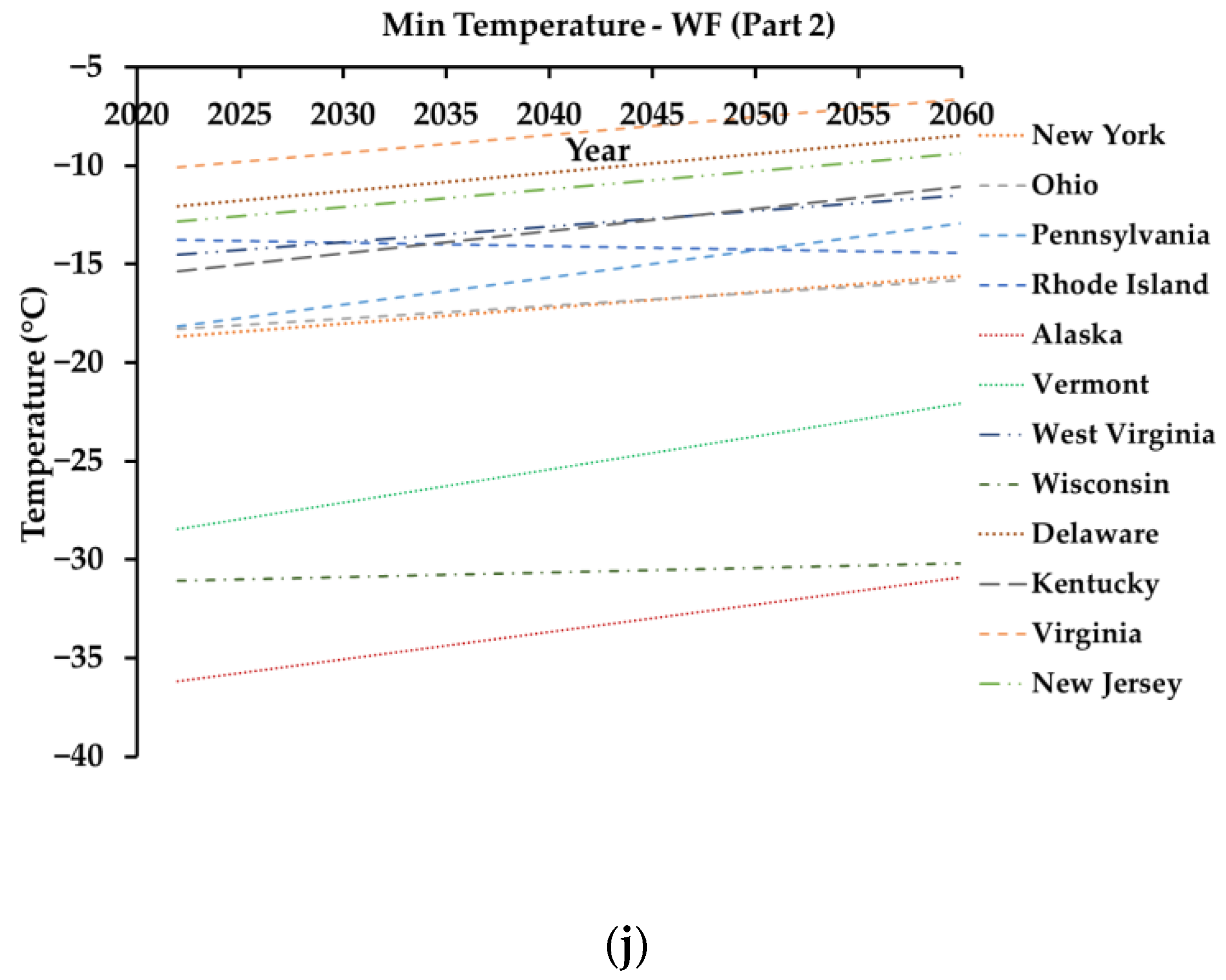
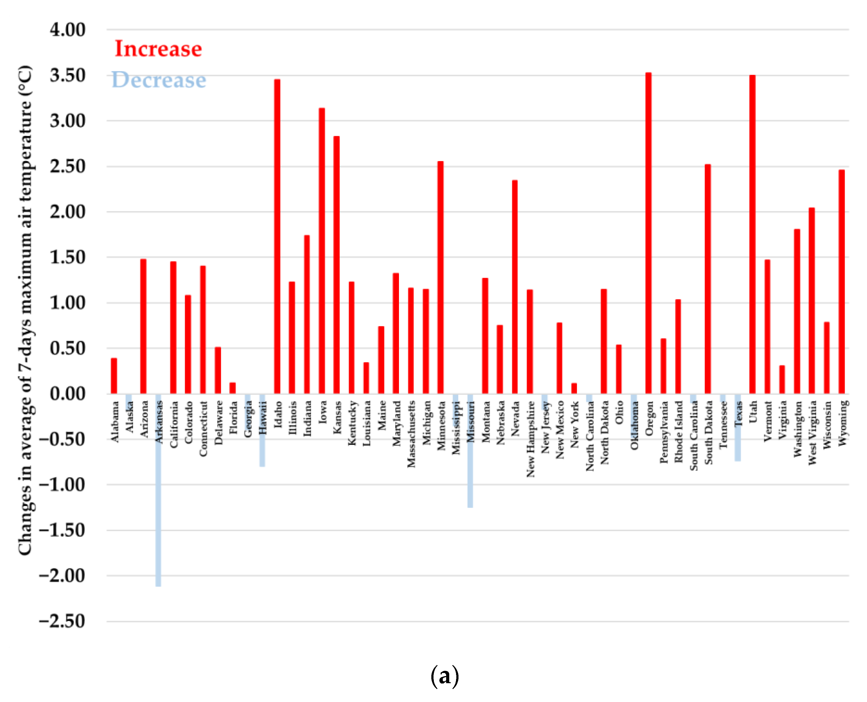
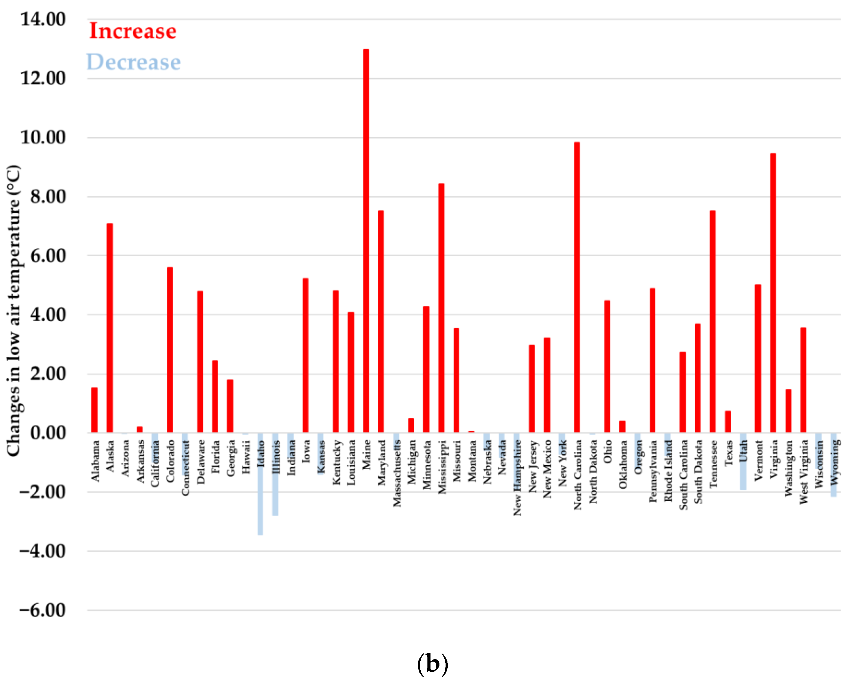
3.1. Prediction of Average 7-Day Maximum and Minimum Air Temperature

The trend in the average 7-day maximum and minimum temperature for each year across the United States is depicted in Figure 1. To clearly distinguish these trends, Figure 1 has been divided into five separate figures for maximum temperature and five separate figures for minimum temperature. Specifically, Figure 1a–e illustrates the trend in the average 7-day maximum temperature from 2022 to 2060 for all states.

Overall, there is an upward trend in maximum temperature across all states. However, the slope of this trend varies: some states experience a steeper increase, while others have a more gradual rise. For example, despite being in distinct climatic zones, Idaho, Oregon, and Utah show a strong increasing trend, whereas Colorado, Hawaii, and North Carolina show a smoother increase.

The annual variation in minimum air temperatures is illustrated in Figure 1f–j. Across most states, the trend for future one-day low air temperatures is increasing, but a few states, including Connecticut and Nevada, exhibit a downward trend.

The difference in average 7-day maximum and minimum air temperatures between two periods—current (1992–2021) and future (2021–2060)—provides insight into temperature changes. Figure 2 illustrates the results of this comparison. Across 38 out of 50 states, the average 7-day maximum temperature during 2021–2060 exceeds that of the present period. Additionally, in 33 states, the minimum air temperature is higher in the future. Notably, in 10 out of the 38 states, the average 7-day maximum temperature has risen by over 2 °C. Given the significant increase in maximum air temperatures in these 10 states and the imposition of stricter limitations due to this rise, ignoring climate change during the infrastructure design stage may result in the selection of inappropriate binders for the designed pavement. Failure to choose suitable binders due to the neglect of climate change can lead to adverse consequences, including a reduction in the pavement’s service life, the need for more frequent maintenance operations, and consequently, increased costs. Oregon experiences the highest increase, with an average 7-day maximum temperature rise of 3.52 °C. Additionally, Figure 2b reveals that in 16 out of the 33 states, minimum air temperatures are predicted to be 4 °C higher in the future. In the state of Maine, the minimum air temperature increase is predicted to be as high as 12.97 °C.

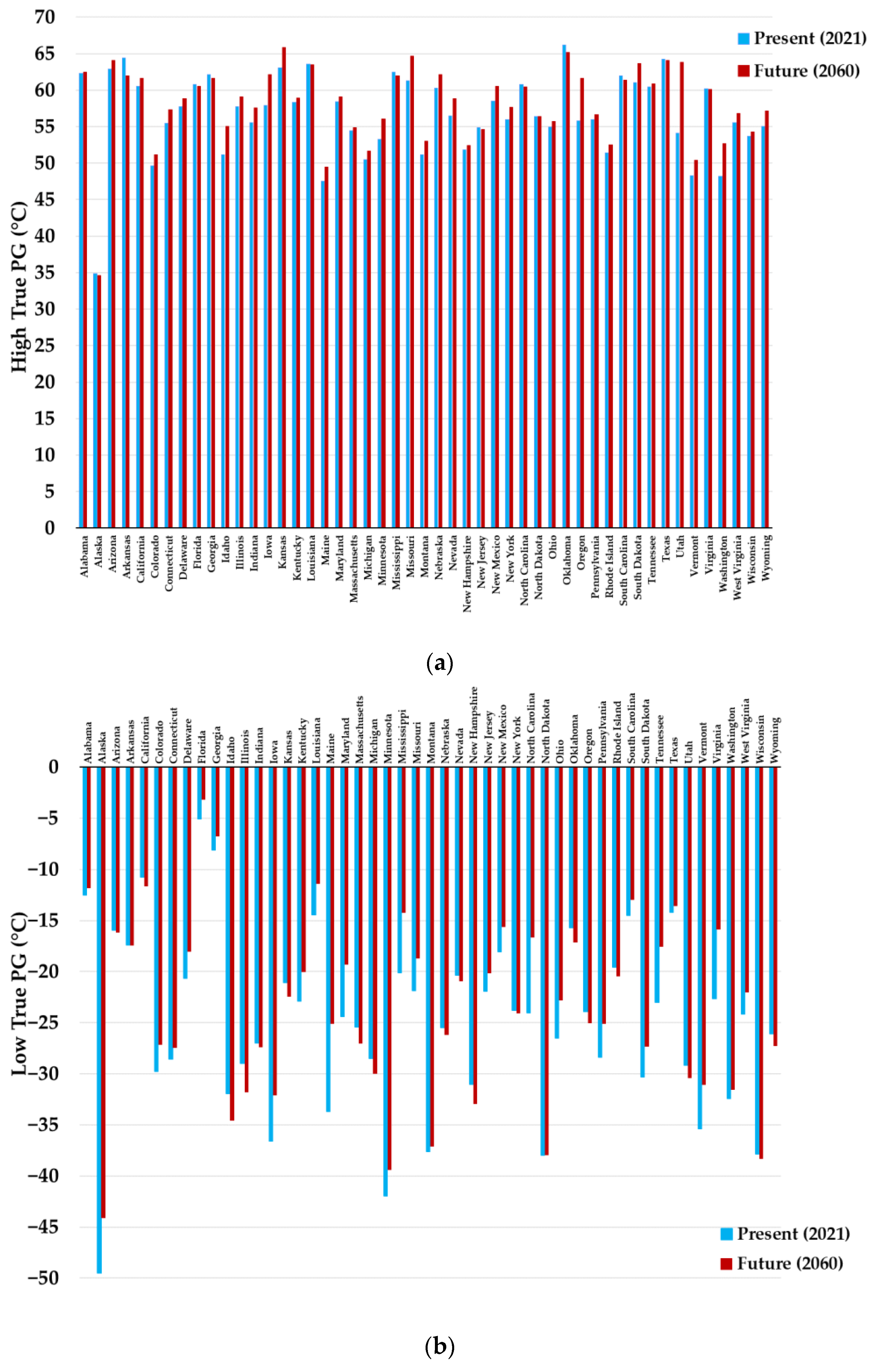
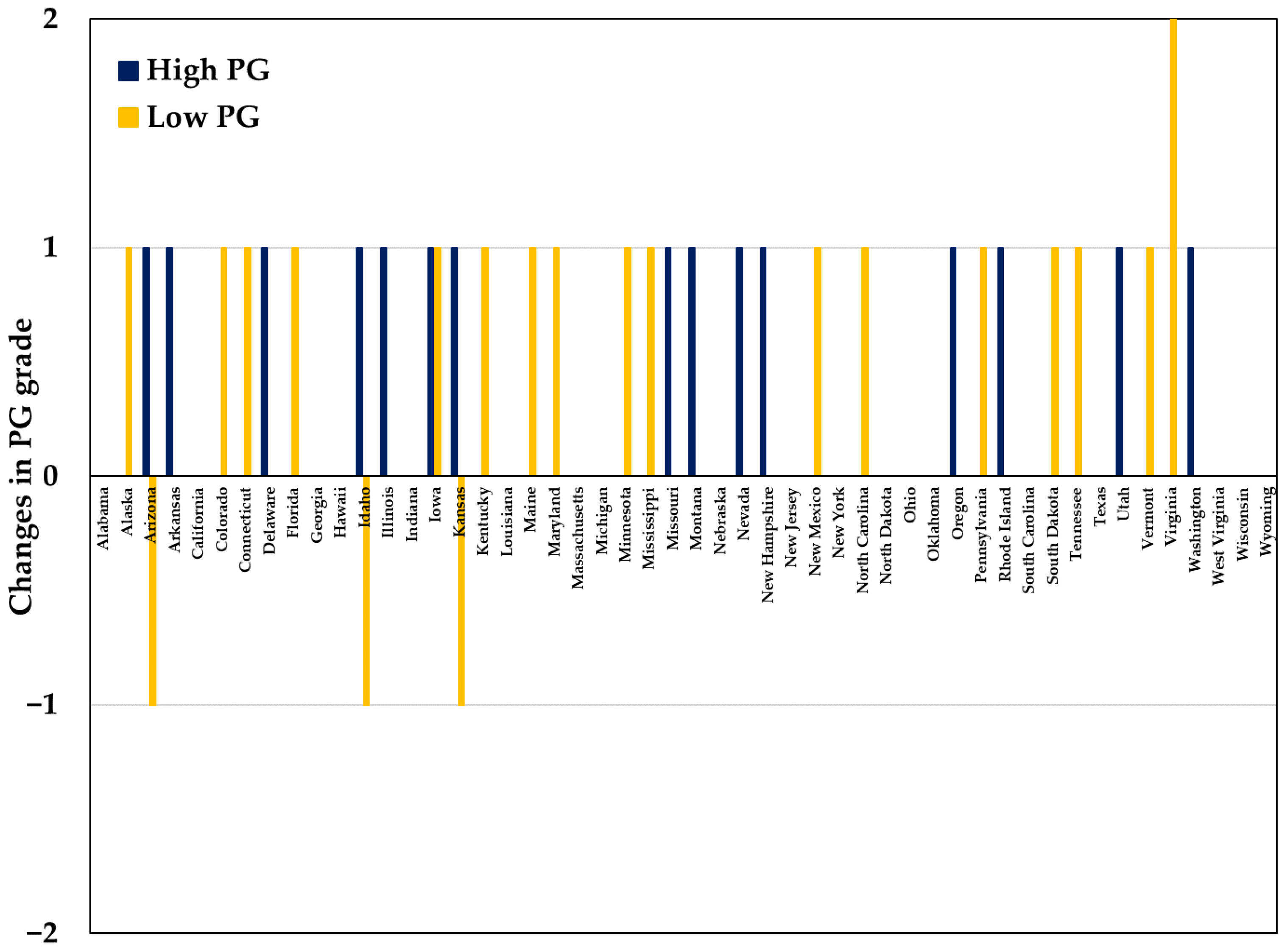
3.2. Binder Performance Grade (PG) Selection

After predicting temperature changes for the future period, the high and low true PG were calculated, as shown in Figure 3. In 36 states, the high true PG values increased, as the same for the low true PG in 30 states. This highlights the impact of changing climate conditions on asphalt pavements for utilizing in the future period. Notably, in states where true PG values have not increased compared to the present period, there has not been a significant decrease either. The decrease in high/low true PG values occurred in states with a downward trend in maximum/minimum temperature time series data from 1992 to 2021.

After calculating the true PG values, PG distribution maps for the United States were plotted for two time periods: 1992 to 2021 (present) and 2021 to 2060 (future), as shown in Figure 4. The PG values presented in these maps represent the requirements for the pavements in each state based on climate condition analyses, without considering the production capabilities of the industry or the effects of traffic speed and volume on binder selection.

To gain a deeper understanding of how changing climate conditions influence the choice of PG, Figure 5 illustrates the impact. As depicted in the figure, the high and low PGs for asphalt will undergo changes in 15 and 20 states, respectively. It is noteworthy to mention that in three states—Arizona, Idaho, and Kansas—the high performance grade has increased, and the low performance grade has decreased. In other words, the temperature performance range between the high and low grades has widened by two grades. In other states, either the high performance grade, the low performance grade, or both have increased. In some states, such as West Virginia, despite significant changes in the average 7-day maximum temperature and minimum air temperature in the future period, there has been no change in the high and low performance grades.

To compare the available PG in the industry with those required in the present and future periods based on the results of this study, Figure 6 is presented. Notably, many of the current PG values fall short of what is needed. To address this, various modifiers are necessary in the base binder to meet the required properties. It is important to note that our analyses rely solely on temperature data, and the specified PG values may differ from those used in the field. These PG values are adjusted based on speed and traffic volume. For instance, consider a high-performance grade currently rated at 76 after accounting for traffic load adjustments. If the average 7-day maximum temperature increases by approximately 2 °C in the future, the required high performance grade could rise by one grade to 82. This impact of changing climatic conditions on PG values must be carefully considered in asphalt pavement design. Ultimately, selecting a PG binder suitable for future climate conditions over a 20- to 30-year design period is crucial.

4. Discussion

The significant impact of changing climate conditions on selecting PG can be a major concern for pavement designers in the future. This study uses time series statistical models to predict future maximum and minimum air temperatures up to 2060. The goal is to understand how these climatic changes will affect the choice of PG in the United States.

By 2060, ten states are projected to see their average 7-day maximum temperatures rise by more than 2 °C. Additionally, 26 states are expected to experience increases of over 1 °C. Overall, 38 out of 50 states are likely to have rising trends in their average 7-day maximum temperatures. Our findings show that Oregon, Utah, and Idaho will face the largest increases in maximum temperature. The results of this study align with findings from Underwood et al. [35], who found that most changes in maximum temperatures across the U.S. from 2040 to 2069 will range between 0 and 4.5 °C. Their study supports our predictions, highlighting a consistent trend due to the overlapping time periods examined.

The low air temperature has increased in 33 states. This increase is more than 4 °C in at least 16 states and more than 2 °C in 23 states. The state of Maine has experienced the highest increase in low air temperature, followed by North Carolina and Virginia. According to the study by Underwood et al. [35], their predictions for minimum temperature, using climate scenarios for the period from 2040 to 2069 range from 0 to 12 °C in most states, which align well with the results of this study. Another noteworthy point is that, except for Hawaii, where both the average 7-day maximum and minimum air temperature are decreasing, no other state has shown a simultaneous decrease in both variables. In 20 states, both maximum and minimum temperatures are increasing.

This study examined how changing climatic conditions affect the calculation of maximum and minimum pavement temperature. We found that high true PG has increased in 36 states, and low true PG has increased in 30 states, while these values have decreased in other states. These shifts in true PG have altered the high and low performance grade in 15 and 20 states, respectively. One crucial finding is that, both in current and future periods, many of the required binders cannot be produced or substituted with other performance grades. For instance, PG70-22 cannot be manufactured or replaced with other grades. As the gap between the required high and low performance grades widens in the future period, this issue needs more consideration.

In this study, for the states of Kansas, Arizona, and Idaho, an increase in the high performance grade and a decrease in the low performance grade have been predicted. The widening gap between the high and low performance grades in these states has resulted in a case where the required PG is not available for the future period. To achieve these performance grades, different modifiers such as crumb rubber (CR), styrene–butadiene–styrene (SBS), polyphosphoric acid (PPA), or gilsonite can be used in the base binder. For example, in a study conducted by Tabatabaee et al. [36], the researchers found that adding 3% CR to the base binder increased the high PG from 58 to 70, and further additions of this modifier to the base binder will increase the high PG even more. In another study, Aflaki and Tabatabaee [12] demonstrated that adding 1%, 2%, and 3% of the SBS modifier to the base binder at a mixing temperature of 160 °C results in an increase of 2.8 °C, 4.4 °C, and 5.8 °C, respectively, in the high true PG value. The results of studies conducted to improve the properties of the binder using the PPA additive have shown that by adding 0.5–1.5% PPA to the base binder, the high-temperature PG increases by one to two grades [37,38]. Ameri et al. [39] investigated the impact of varying percentages of gilsonite as a modifier on two binder samples, specifically PG58-22 and PG64-22. Their findings revealed that incorporating 4%, 8%, and 12% gilsonite into the binder resulted in an increase in the high-temperature PG by 1 to 3 grades, respectively. Conversely, these gilsonite additions did not significantly enhance the low-temperature PG, with improvements in the low true PG ranging from 1 to 5 °C. Notably, the effect of the gilsonite modifier on the PG64-22 binder differed, demonstrating a lesser increase in high true PG but a more pronounced enhancement in low true PG. The energy consumption and CO₂ emissions while using these modifiers must be taken into account.

Table 4. Energy consumption and CO₂ emissions for producing 1 ton of different modifiers.

Parameters	CR [40]	SBS [40]	PPA [41,42]	Gilsonite [43]
Energy consumption (kWh)	639	21,274	10,000–20,000	500–800
CO2 emissions (kg)	510	4015.43	2500–4500	100–150

presents the energy consumption and CO₂ emissions associated with producing 1 ton of these modifiers.

Producing 1 ton of asphalt requires approximately 50 kg of binder. According to commonly used percentages in previous studies [36,37,38,39,40], modifying the base binder typically requires approximately 20% CR, 5% SBS, 1.5% PPA, or 8% gilsonite modifiers. Consequently, to produce 1 ton of asphalt, 10 kg of CR, 2.5 kg of SBS, 0.75 kg of PPA, or 4 kg of gilsonite should be used. To evaluate the environmental impacts, a comparison of the energy consumption and CO₂ emissions among the modifiers is provided in

Table 5. Comparison of energy consumption and CO₂ emissions for producing 1 ton of asphalt with different modifiers.

Modifiers	Weight (kg)	Energy Consumption (kWh)	CO2 Emissions (kg)
CR (20%)	10	6.39	5.10
SBS (5%)	2.5	53.18	10.03
PPA (1.5%)	0.75	7.50–15.00	1.87–3.37
Gilsonite (8%)	4	2.00–3.20	0.40–0.60

. As shown in Table 4, producing 1 ton of CR consumes 639 kWh of energy and emits 510 kg of CO₂, whereas producing 1 ton of SBS consumes 21,274 kWh of energy and emits 4015.43 kg of CO₂. As a result, producing 10 kg of CR requires 6.39 kWh of energy, while producing 2.5 kg of SBS requires 53.185 kWh. Additionally, the CO₂ emissions for producing 1 ton of asphalt, considering the specified percentages of CR and SBS modifiers, are 5.1 kg and 10.03 kg, respectively. This example illustrates that using CR as a modifier requires less energy and results in lower CO₂ emissions compared to SBS. To put this into perspective, the average monthly electricity consumption for a household in urban areas is approximately 75 kWh [44]. Thus, the average daily electricity consumption for a household is approximately 2.5 kWh. By using CR instead of SBS to modify the base binder in asphalt production, 46.795 kWh of energy per ton of asphalt can be saved. This amount of saved energy is enough to supply the daily energy needs of 18 to 19 households. This example underscores the significance of taking into account both energy consumption and CO₂ emissions when modifying the available PG to attain the desired PG with properties suitable for the prevailing climatic conditions.

As mentioned, achieving the required characteristics of the binder may necessitate the use of modifiers. In this context, simultaneously examining life cycle assessment (LCA) and life cycle cost analysis (LCCA) is challenging. When adding a modifier to the binder, the benefits should be weighed against the drawbacks. Some benefits of adding a modifier include increased durability, extended service life of the pavement, and reduced maintenance frequency. However, the drawbacks may include economic and environmental issues, such as additional initial costs for producing modified binder, energy consumption, and CO₂ emissions. Underwood et al. [35] assessed the economic impacts of using correct versus incorrect asphalt grades for flexible pavements across different roadway types. For 2040, the projected costs in the United States are USD 19.0 billion for RCP 4.5 and USD 26.3 billion for RCP 8.5. By 2070, these costs are estimated to increase to USD 21.8 billion for RCP 4.5 and USD 35.8 billion for RCP 8.5. These findings underscore the vital importance of selecting the appropriate asphalt binder grade to minimize pavement costs. Sharma et al. [45] estimated the early maintenance demands expected as a result of climate change. Frequent maintenance contributes to additional traffic delay emissions and increased costs. Their study found that early maintenance in El Paso and Austin, Texas, led to 70 tons of CO₂ emissions per day and USD 100,000 in costs per maintenance day. Consequently, conducting an LCA for different adaptation strategies is crucial to selecting the most effective approach. Incorporating changes in binder grades into LCCA and LCA requires a comprehensive understanding of both the economic and environmental implications. While modified binders may increase initial costs and environmental impacts during production, their improved performance can lead to significant savings and reduced environmental footprints over the pavement’s life cycle. By integrating LCCA and LCA methodologies, construction and maintenance strategies can be optimized to enhance serviceability and durability while minimizing emissions.

5. Conclusions

The analysis presented in this study underscores the significant impact of global warming on binder performance grading (PG) in the United States, highlighting key sustainability challenges. Based on the findings of this research, the following main conclusions can be drawn:

• Using time series models to forecast temperature changes up to 2060, substantial increases in both maximum and minimum air temperatures across the majority of states are projected. Specifically, 38 out of 50 states are expected to experience rising maximum temperatures, with Oregon, Utah, and Idaho facing the most significant increases. Concurrently, 33 states are anticipated to see higher minimum temperatures, notably in Maine, North Carolina, and Virginia.
• The widening gap between the required high and low PG values presents a critical challenge, as some essential binders may not be producible or substitutable with other grades. This situation necessitates the use of modifiers to achieve the desired PG properties, bringing additional considerations regarding energy consumption and CO₂ emissions. While modified binders may incur higher initial costs and environmental impacts, their improved performance can lead to long-term savings and reduced environmental footprints.
• By integrating life cycle cost analysis (LCCA) and life cycle assessment (LCA) methodologies, this study provides a comprehensive understanding of the economic and environmental implications of various binder modifications. This integrated approach is essential for optimizing construction and maintenance strategies to enhance the durability and serviceability of pavements while minimizing emissions.
• This study emphasizes the need for proactive adaptation strategies in pavement design to address the mounting impacts of climate change, ensuring the long-term resilience of infrastructure in the United States.

Building on the insights gleaned from the findings and discussions of this study, future research could delve into the following areas of consideration: (1) Exploring the selection of suitable modifiers and determining their optimal amount to attain the desired PG value in states where suitable PG options are lacking due to predicted climate changes and sustainability concerns. (2) While this study utilized a statistical time series model for temperature prediction, future investigations could explore alternative climate models incorporating diverse socio-economic scenarios. Such efforts may enhance the understanding of future temperature patterns, reducing the risk of temperature overestimation or underestimation. (3) Temperature and precipitation are pivotal factors impacting pavement materials and design. Consequently, it is imperative to assess the individual contributions of these climate variables to pavement design under future climate conditions. (4) Future traffic patterns exert a significant influence on pavement infrastructure. Thus, it is essential to evaluate the interaction between climate factors and future traffic to inform PG selection effectively.

6. Limitations and Assumptions

Certain assumptions and limitations were considered in conducting this study: (1) To predict the maximum and minimum temperatures in each state, data from a single weather station were used. For a more accurate examination of PG binder changes, it would be beneficial to utilize data from a larger number of weather stations in each state. Consequently, the analyses presented primarily highlight the importance of temperature changes in the future period within the vicinity of the weather station considered in this study. (2) The PG values presented in this study represent the requirements for pavements in each state based on climate condition analyses, without taking into account the production capabilities of the industry or the effects of traffic conditions on PG selection. (3) This study focused solely on the effect of temperature changes on the PG value, disregarding the effects of other climate factors or the impact of binder aging on PG changes.

References

1. Duchenne-Moutien, R.A.; Neetoo, H. Climate change and emerging food safety issues: A review. J. Food Prot. 2021, 84, 1884–1897. [Google Scholar] [CrossRef] [PubMed]
2. Naseri, H.; Ehsani, M.; Golroo, A.; Moghadas Nejad, F. Sustainable pavement maintenance and rehabilitation planning using differential evolutionary programming and coyote optimisation algorithm. Int. J. Pavement Eng. 2022, 23, 2870–2887. [Google Scholar] [CrossRef]
3. Satterthwaite, D. The implications of population growth and urbanization for climate change. Environ. Urban. 2009, 21, 545–567. [Google Scholar] [CrossRef]
4. Oreggioni, G.D.; Ferraio, F.M.; Crippa, M.; Muntean, M.; Schaaf, E.; Guizzardi, D.; Solazzo, E.; Duerr, M.; Perry, M.; Vignati, E. Climate change in a changing world: Socio-economic and technological transitions, regulatory frameworks and trends on global greenhouse gas emissions from EDGAR v. 5.0. Glob. Environ. Chang. 2021, 70, 102350. [Google Scholar] [CrossRef]
5. Ekwurzel, B.; Boneham, J.; Dalton, M.W.; Heede, R.; Mera, R.J.; Allen, M.R.; Frumhoff, P.C. The rise in global atmospheric CO2, surface temperature, and sea level from emissions traced to major carbon producers. Clim. Chang. 2017, 144, 579–590. [Google Scholar] [CrossRef]
6. Raftery, A.E.; Zimmer, A.; Frierson, D.M.; Startz, R.; Liu, P. Less than 2 C warming by 2100 unlikely. Nat. Clim. Chang. 2017, 7, 637–641. [Google Scholar] [CrossRef] [PubMed]
7. Anderson, D.A.; Christensen, D.W.; Bahia, H.U.; Dongre, R.; Sharma, M.G.; Antle, C.E.; Button, J. Binder Characterization and Evaluation, Volume 3: Physical Characterization; Strategic Highway Research Program, National Research Council: Washington, DC, USA, 1994. [Google Scholar]
8. Bahia, H.U.; Anderson, D.A. Strategic highway research program binder rheological parameters: Background and comparison with conventional properties. Transp. Res. Rec. 1995, 8, 32–39. [Google Scholar]
9. Kennedy, T.W.; Huber, G.A.; Harrigan, E.T.; Cominsky, R.J.; Hughes, C.S.; Von Quintus, H.; Moulthrop, J.S. Superior Performing Asphalt Pavements (Superpave): The Product of the SHRP Asphalt Research Program; National Research Council: Washington, DC, USA, 1994. [Google Scholar]
10. Petersen, J.C.; Robertson, R.E.; Branthaver, J.F.; Harnsberger, P.M.; Duvall, J.J.; Kim, S.S.; Anderson, D.A.; Christiansen, D.W.; Bahia, H.U. Binder Characterization and Evaluation; National Research Council: Washington, DC, USA, 1994; Volume 1. [Google Scholar]
11. Yusoff, N.I.; Shaw, M.T.; Airey, G.D. Modelling the linear viscoelastic rheological properties of bituminous binders. Constr. Build. Mater. 2011, 25, 2171–2189. [Google Scholar] [CrossRef]
12. Aflaki, S.; Tabatabaee, N. Proposals for modification of Iranian bitumen to meet the climatic requirements of Iran. Constr. Build. Mater. 2009, 23, 2141–2150. [Google Scholar] [CrossRef]
13. Viola, F.; Celauro, C. Effect of climate change on asphalt binder selection for road construction in Italy. Transp. Res. Part D Transp. Environ. 2015, 37, 40–47. [Google Scholar] [CrossRef]
14. Delgadillo, R.; Arteaga, L.; Wahr, C.; Alcafuz, R. The influence of climate change in Superpave binder selection for Chile. Road Mater. Pavement Des. 2020, 21, 607–622. [Google Scholar] [CrossRef]
15. Swarna, S.T.; Hossain, K. Asphalt binder selection for future Canadian climatic conditions using various pavement temperature prediction models. Road Mater. Pavement Des. 2023, 24, 447–461. [Google Scholar] [CrossRef]
16. Sheng, J.; Miao, Y.; Wang, L. An Assessment of the Impact of Climate Change on Asphalt Binder Selection in East China Based on the ARIMA Model. Sustainability 2023, 15, 15667. [Google Scholar] [CrossRef]
17. El Haloui, Y.; Sepaspour, R.; Hajikarimi, P.; Moghadas Nejad, F.; Fakhari Tehrani, F.; Absi, J. Adoption of Asphalt Binder Performance Grades for Morocco Considering Climate Change. Int. J. Civ. Eng. 2023, 21, 1061–1075. [Google Scholar] [CrossRef]
18. Hulme, M.; Brown, O. Portraying climate scenario uncertainties in relation to tolerable regional climate change. Clim. Res. 1998, 10, 1–4. [Google Scholar] [CrossRef]
19. Hulme, M.; Viner, D. A climate change scenario for the tropics. Clim. Chang. 1998, 39, 145–176. [Google Scholar] [CrossRef]
20. Zebarjadian, F.; Dolatabadi, N.; Zahraie, B.; Yousefi Sohi, H.; Zandi, O. Triple coupling random forest approach for bias correction of ensemble precipitation data derived from Earth system models for Divandareh-Bijar Basin (Western Iran). Int. J. Climatol. 2024, 44, 2363–2390. [Google Scholar] [CrossRef]
21. Sarraf, A.; Vahdat, S.F.; Behbahaninia, A. Relative humidity and mean monthly temperature forecasts in Ahwaz Station with ARIMA model in time series analysis. In Proceedings of the International Conference on Environment and Industrial Innovation IPCBEE, Frankfurt, Germany, 28–30 June 2011; IACSIT Press: Singapore, 2011; Volume 12. [Google Scholar]
22. Nury, A.H.; Koch, M.; Alam, M.J. Time series analysis and forecasting of temperatures in the sylhet division of bangladesh. In Proceedings of the 4th International Conference on Environmental Aspects of Bangladesh (ICEAB), Kitakyushu, Japan, 24–26 August 2013; pp. 24–26. [Google Scholar]
23. Papacharalampous, G.; Tyralis, H.; Koutsoyiannis, D. Predictability of monthly temperature and precipitation using automatic time series forecasting methods. Acta Geophys. 2018, 66, 807–831. [Google Scholar] [CrossRef]
24. Box, G.E.; Jenkins, G.M.; Reinsel, G.C.; Ljung, G.M. Time Series Analysis: Forecasting and Control; John Wiley Sons: Hoboken, NJ, USA, 2015. [Google Scholar]
25. Lu, P.; Tolliver, D. Pavement treatment short-term effectiveness in IRI change using long-term pavement program data. J. Transp. Eng. 2012, 138, 1297–1302. [Google Scholar] [CrossRef]
26. Carvalho, R.; Ayres, M.; Shirazi, H.; Selezneva, O.; Darter, M. Impact of Design Features on Pavement Response and Performance in Rehabilitated Flexible and Rigid Pavements; Turner-Fairbank Highway Research Center: McLean, VA, USA, 2011. [Google Scholar]
27. Elkins, G.E.; Schmalzer, P.N.; Thompson, T.; Simpson, A. Long-Term Pavement Performance Information Management System: Pavement Performance Database User Reference Guide; Turner-Fairbank Highway Research Center: McLean, VA, USA, 2003. [Google Scholar]
28. Drumm, E.C.; Meier, R. LTPP Data Analysis: Daily and Seasonal Variations in Insitu Material Properties; Transportation Research Board, National Research Council: Washington, DC, USA, 2003. [Google Scholar]
29. Karamouz, M.; Nazif, S.; Falahi, M. Hydrology and Hydroclimatology: Principles and Applications; CRC Press: Boca Raton, FL, USA, 2012. [Google Scholar]
30. Salas, J.D.; Delleur, J.; Yevjevich, W.V.; Lane, W.L. Applied Modeling of Hydrological Time Series; Water Resources Publication: Chicago, IL, USA, 1988. [Google Scholar]
31. Box, G.E.; Cox, D.R. An analysis of transformations. J. R. Stat. Soc. Ser. B Stat. Methodol. 1964, 26, 211–243. [Google Scholar] [CrossRef]
32. Pregnolato, M.; Ford, A.; Wilkinson, S.M.; Dawson, R.J. The impact of flooding on road transport: A depth-disruption function. Transp. Res. Part D Transp. Environ. 2017, 55, 67–81. [Google Scholar] [CrossRef]
33. Akaike, H. A new look at the statistical model identification. IEEE Trans. Autom. Control 1974, 19, 716–723. [Google Scholar] [CrossRef]
34. Anderson, R.L. Distribution of the serial correlation coefficient. Ann. Math. Stat. 1942, 13, 1–3. [Google Scholar] [CrossRef]
35. Underwood, B.S.; Guido, Z.; Gudipudi, P.; Feinberg, Y. Increased costs to US pavement infrastructure from future temperature rise. Nat. Clim. Chang. 2017, 7, 704–707. [Google Scholar] [CrossRef]
36. Tabatabaee, N.; Tabatabaee, H.A.; Sabouri, M.R.; Teymourpour, P. Evaluation of performance grading parameters for crumb rubber modified asphalt binders and mixtures. In Advanced Testing and Characterization of Bituminous Materials, Two Volume Set; CRC Press: Boca Raton, FL, USA, 2009; pp. 613–622. [Google Scholar]
37. Ghabchi, R.; Rani, S.; Zaman, M.; Ali, S.A. Effect of WMA additive on properties of PPA-modified asphalt binders containing anti-stripping agent. Int. J. Pavement Eng. 2021, 22, 418–431. [Google Scholar] [CrossRef]
38. Fee, D.; Maldonado, R.; Reinke, G.; Romagosa, H. Polyphosphoric acid modification of asphalt. Transp. Res. Rec. 2010, 2179, 49–57. [Google Scholar] [CrossRef]
39. Ameri, M.; Mansourian, A.; Ashani, S.S.; Yadollahi, G. Technical study on the Iranian Gilsonite as an additive for modification of asphalt binders used in pavement construction. Constr. Build. Mater. 2011, 25, 1379–1387. [Google Scholar] [CrossRef]
40. Wang, Q.Z.; Wang, N.N.; Tseng, M.L.; Huang, Y.M.; Li, N.L. Waste tire recycling assessment: Road application potential and carbon emissions reduction analysis of crumb rubber modified asphalt in China. J. Clean. Prod. 2020, 249, 119411. [Google Scholar] [CrossRef]
41. Pradhan, K.C.; Mishra, B.; Mohapatra, S.M. Investigating the relationship between economic growth, energy consumption, and carbon dioxide (CO2) emissions: A comparative analysis of South Asian nations and G-7 countries. Clean Technol. Environ. Policy 2024, 1–9. [Google Scholar] [CrossRef]
42. Emenekwe, C.C.; Onyeneke, R.U.; Nwajiuba, C.U.; Anugwa, I.Q.; Emenekwe, O.U. Determinants of consumption-based and production-based carbon emissions. Environ. Dev. Sustain. 2023, 1–37. [Google Scholar] [CrossRef]
43. Al Hawesah, H.; Sadique, M.; Harris, C.; Al Nageim, H.; Stopp, K.; Pearl, H.; Shubbar, A. A review on improving asphalt pavement service life using gilsonite-modified bitumen. Sustainability 2021, 13, 6634. [Google Scholar] [CrossRef]
44. Hajikarimi, P.; Shariati, S.; Rahi, M.; Kazemi, R.; Nejad, F.M.; Fini, E.H. Enhancing the economics and environmental sustainability of the manufacturing process for air-blown bitumen. J. Clean. Prod. 2021, 323, 128978. [Google Scholar] [CrossRef]
45. Sharma, M.; Inti, S.; Tandon, V.; Byreddy, H. Economical and environmental impact of climate change on Texas pavements. In Proceedings of the TRB 99th Annual Meeting, Washington, DC, USA, 12–16 January 2020; Walter E. Washington Convention Center: Washington, DC, USA, 2020; pp. 12–16. [Google Scholar]
Figure 1. The predicted trend of changes in the average 7-day maximum air temperature for (a) WNF, (b) DNF, (c) DF, (d) WF-Part 1, (e) WF-Part 2, and minimum air temperature for (f) WNF, (g) DNF, (h) DF, (i) WF-Part 1, and (j) WF-Part 2 for the future period.
Infrastructures 09 00109 g001aInfrastructures 09 00109 g001bInfrastructures 09 00109 g001cInfrastructures 09 00109 g001d
Figure 2. Changes in (a) average 7-day maximum and (b) minimum air temperature in the future compared to the current period.
Infrastructures 09 00109 g002aInfrastructures 09 00109 g002b
Figure 3. (a) High and (b) low true performance grade (PG) values for different states.
Infrastructures 09 00109 g003
Figure 4. PG distribution maps (without considering traffic conditions) for (a) present (1992–2021) and (b) future period (2022–2060).
Infrastructures 09 00109 g004
Figure 5. Changes in high and low performance grade in the future period compared to the current period.
Infrastructures 09 00109 g005
Figure 6. Available and required PG comparison in the present and future periods.
Infrastructures 09 00109 g006