Inertial Methodology for the Monitoring of Structures in Motion Caused by Seismic Vibrations

Abstract

This paper presents a non-invasive methodology for structural health monitoring (SHM) integrated with inertial sensors and signal conditioning techniques. The proposal uses the signal of an IMU (inertial measurement unit) tri-axial accelerometer and gyroscope to continuously measure the displacements of a structure in motion due to seismic vibrations. A system, called the “Inertial Displacement Monitoring System” or “IDMS”, is implemented to attenuate the signal error of the IMU with methodologies such as a Kalman filter to diminish the influence of white noise, a Chebyshev filter to isolate the frequency values of a seismic motion, and a correction algorithm called zero velocity observation update (ZVOB) to detect seismic vibrations and diminish the influence of external perturbances. As a result, the IDMS is a methodology developed to measure displacements when a structure is in motion due to seismic vibration and provides information to detect failures opportunely.

1. Introduction

Implementing structural health monitoring (SHM) technologies to measure the condition of a structure when subjected to seismic motion is a topic of interest for public safety, particularly in seismic regions. Proper failure detection generates opportunities for adequate maintenance and the understanding of what generates a fracture or collapse in structures such as buildings, tunnels, bridges, or the included mechanical structural systems such as tanks, wind turbines, and aerospace composites [1,2].

Currently, there are different approaches to performing SHM and obtaining information about a structure’s condition when it is subjected to an earthquake. Research such as implementing cameras to obtain images and video is a proposal complemented by training neural networks, where the information from databases is used to detect irregularities [3,4,5]. These techniques implement pattern recognition techniques that seek to imitate how the human brain works [6,7]. Additionally, they are trained with vibration signals and register the information at different levels or structural states. However, neural networks and other non-deterministic models require high computational resources, and they are susceptible to noise generated in the environment, which can make it difficult to monitor the process for structures in monitoring networks [8,9,10].

Other research has suggested the use of optical sensors in an effort to detect cracks, delamination, or fractures [11,12,13], or implementing laser scanning techniques capable of detecting displacements and structural deformations [14,15]. These technologies are non-invasive and provide monitoring of structures, where digitalized images detect specified parameters that serve as a reference for the system. Hence, as optical sensors and laser scanning techniques provide useful information to monitor structural health, light reflection and the illumination intensity can cause measurement errors due to the changing nature of the environment. In addition, optical sensors are required to be isolated from the vibrations affecting the structure, and it is necessary to place them under proper light conditions to avoid measurement errors [16,17,18].

Furthermore, some researchers have considered accelerometers to perform SHM, because they can measure under dynamic conditions and provide vibration measurements, and this information is used to calculate displacements in structures. However, some systems have problems synchronizing the measured data when using digital accelerometers; there is an inherent drift in inertial sensors [19,20]. Hence, some of the proposals have used probabilistic or machine learning techniques. Consequently, most inertial systems are used as a complement to a more robust system to compensate for measurement errors [21,22].

Although the mentioned techniques provide valuable data on a structure’s condition, they are susceptible to environmental interferences and have present difficulties monitoring when atypical behavior influences the structure. As a result, suitable detection of fractures in structures due to the displacements produced by seismic motion is still a challenge.

This paper presents the use of an accelerometer in conjunction with a gyroscope in an “Inertial Measurement Unit” IMU inertial sensor, where the acquired signal of the movements in the structure is analyzed and used to calculate the displacement with the signal conditioning phase [23,24,25]. As microelectromechanical systems (MEMS) can be placed at different points on a structure in a non-invasive configuration, the system provides information about the structure to perform a non-destructive evaluation.

The methodology “Inertial Displacement Monitoring System” or IDMS measures the displacements in a two-degrees-of-freedom (DoF) structural system placed on a shaking table that simulates the seismic motion of primary waves (P-waves) in a horizontal plane. The system implements the IMU’s accelerometer and gyroscope placed at the top of one of the links of the structure and performs signal conditioning using a Kalman filter and a proposed zero velocity observation update (ZVOB) correction algorithm. The principle of the system, called the inertial displacement monitoring system “IDMS”, is shown in Figure 1 and will be explained in Section 4.

The main contributions of this paper are summarized as follows:

• Continuous monitoring and measurement of structure displacement caused by seismic vibration.
• An inertial system is implemented to perform SHM under seismic vibrations and provide information to perform a non-destructive evaluation.
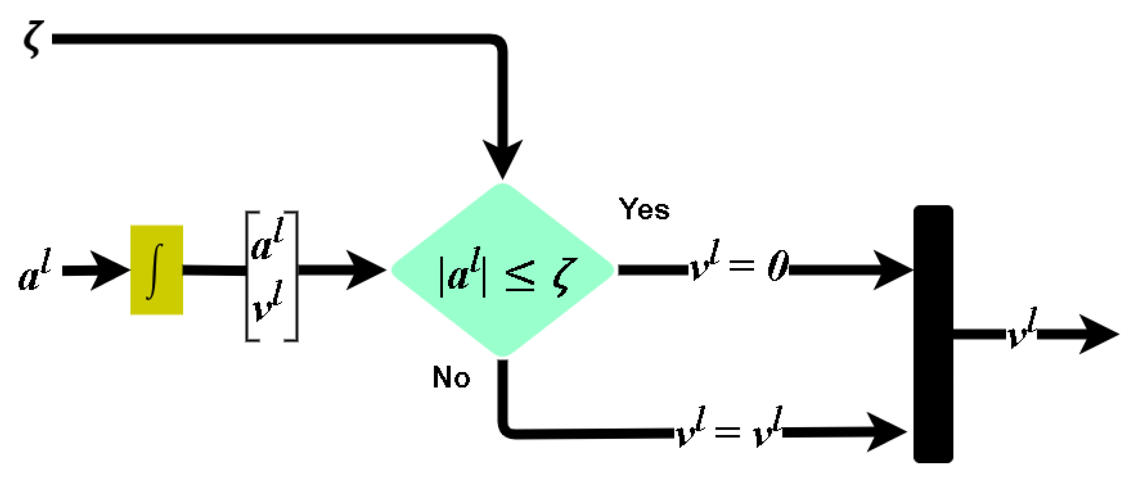
• Correction algorithm ZVOB: ZVOB is a robust technique that evaluates whether a body is still in motion or in a steady-state phase.
• Drift reduction: error caused by drift due to the accelerometer is attenuated to increase the precision of measurements.
• Frequency analysis of a structure to measure the displacement when it is excited by seismic vibrations.

This paper is organized as follows: Section 2, Inertial Sensor Computations, presents equations and principles of an inertial system, describing the reference frame and how its position is calculated. Section 3, Signal Conditioning, presents the filter and correction algorithms implemented to attenuate the error and measure under seismic vibratory conditions. Section 4, Inertial Displacement Monitoring System, describes the principle of the IDMS and contains an description of the methodology; additionally, it includes a block diagram with the elements that compose the system presented in this paper. Section 5, Experimentation, explains the developed experiments and the conditions that demonstrate the system’s effectiveness. Section 6, Results, gives an analysis of the obtained results and a statistical interpretation of the data. Section 7, Discussion, is where the system results are compared to other works. Section 8, Conclusions, summarizes the main points and presents future research.

2. Inertial Sensor Computations

2.1. Local Level Reference Frame

The IDMS methodology processes MEMS inertial sensor signals acquired by a data acquisition system connected to a computer and calculates the structural displacement through mathematical methods. The implemented IMU is in a strapdown configuration, where the three accelerometers are placed on a printed circut board (PCB) with their center of gravity (cg) aligned [26]. Therefore, the IMU is mounted on one of the sides of the structure and aligns with of the axes of the simulated movement. In Figure 2 is shown a diagram of the IMU with the orientation of three accelerometers mounted on the structure.

All the measurements and experiments of the IDMS are located in a local level reference frame l-frame. The l-frame presents the object of interest in a non-accelerating and non-rotating set of axes configuration known as ENU (East, North, Up), where the z-axis points up and is aligned with the Earth’s gravity [27,28]. The IMU sensor is placed to measure the different displacements caused by seismic vibrations and so that it will maintain the same orientation in the same reference frame.

2.2. Velocity and Position

In an inertial system where accelerometer measurements are used to calculate a body’s position, it is required to condition the sensor’s information considering the Earth’s gravity g and Coriolis force $\mathsf{\Omega }$ [29].

The Coriolis effect $\mathsf{\Omega }$ is a deflective force created by the Earth’s rotation, affecting bodies on its surface. An inertial system can measure this with a gyroscope contained in an IMU. The IDMS system includes a gyroscope for measuring the angular velocity caused by the Coriolis force [30]. Hence, the signal acquired by the gyroscope ${\mathit{\omega }}^l$ is a combination of the Coriolis effect $\mathsf{\Omega }$ and the sensor’s angular velocity in ${\omega }_x^l$, ${\omega }_y^l$ and ${\omega }_z^l$.

$${\mathit{\omega }}^{\mathit{l}}=\left[\begin{array}{c}{\omega }_x^l\\ {\omega }_y^l\\ {\omega }_z^l\end{array}\right]+\left[\begin{array}{c}{\mathsf{\Omega }}_x\\ {\mathsf{\Omega }}_y\\ {\mathsf{\Omega }}_z\end{array}\right]=(\mathit{\omega }+\mathsf{\Omega })$$

(1)

In a navigation body, the acceleration is affected by a radial force produced by the angular velocities contained in the ${\mathit{\omega }}^{\mathit{l}}$ cross product with the sensor’s velocity ${\mathbf{v}}^l$ and by the gravitational acceleration ${\mathbf{g}}^l$ [31]. Therefore, to calculate the inertial acceleration of the sensor, it is necessary to isolate the accelerometer’s signal from the mentioned external forces, as demonstrated below in Equation (2).

$${\mathbf{a}}_I^l=\left[\begin{array}{c}{a}_x^l\\ a_y^l\\ a_z^l\end{array}\right]={\mathbf{a}}^l-({\mathit{\omega }}^{\mathit{l}}+\mathsf{\Omega })\times {\mathbf{v}}^l-{\mathbf{g}}^l$$

(2)

Afterward, integration is applied to the data in order to obtain the displacement, once to compute from acceleration to velocity and again to calculate position with velocity.

$${\mathbf{v}}^l\left(n\right)={\int }_{n-1}^n{\mathbf{a}}_I^{l}dt\approx {\mathbf{v}}^l[n-1]+{\mathbf{a}}_I^l\left[n\right]\mathsf{\Delta }t$$

(3)

$${\mathbf{p}}^l\left(n\right)={\int }_{n-1}^n{\mathbf{v}}^{l}dt\approx {\mathbf{p}}^l[n-1]+{\mathbf{v}}^l\left[n\right]\mathsf{\Delta }t$$

(4)

where ${\mathit{v}}^l$ and ${\mathit{p}}^l$ are vectors presenting the velocity and position in the three axes. Hence, calculating the position only with the equations presented in this section is insufficient to provide a precise measurement of the shaking table movement. Therefore, a signal conditioning phase is implemented to diminish the error and attenuate drift.

3. Signal Conditioning

Inertial sensor computations are a fundamental part of the system for estimating displacement. Thus, as in most inertial systems, there is an inherent bias in the sensors and a multi-factorial drift in the system. Consequently, inconsistencies exist between the obtained measurements and the calculations performed, even in ideal conditions.

Therefore, a filtering phase and a correction algorithm must be integrated to attenuate the noise signals present in the sensors arrangement.

3.1. Kalman Filter

In the IDMS, a Kalman filter attenuates the white noise in accelerometer-acquired signals, along with the estimated velocity and position [32,33]. These data are contained in the measurement vector X as follows:

$$\mathbf{X}=\left[\begin{array}{c}{\mathbf{v}}^l\\ {\mathbf{p}}^l\end{array}\right]$$

(5)

It is important to remember that ${\mathit{v}}^l$ and ${\mathit{p}}^l$ are vectors with data from the three axes, as Equations (3) and (4) show.

Subsequently, the Kalman filter initiates with an a priori state, calculating the prediction state correction vector $\widehat{{\mathbf{x}}_n^{-}}$, as shown below:

$$\widehat{{\mathit{x}}_n^{-}}={\mathbf{F}}_{n-1}\widehat{{\mathbf{x}}_{n-1}}$$

(6)

where ${\mathbf{F}}_{n-1}$ is the state’s transition matrix and $\widehat{{\mathbf{x}}_{n-1}}$ represents the previous state’s correction vector. Afterward, the error matrix covariance P is calculated, which considers the noise covariance ${\mathbf{Q}}_{n-1}$ of the system and ${\mathbf{F}}_{n-1}$. Hence, P is computed as

$${\mathbf{P}}_n^{-}={\mathbf{F}}_{n-1}{\mathbf{P}}_{n-1}{\left({\mathbf{F}}_{n-1}\right)}^T+{\mathbf{Q}}_{n-1}$$

(7)

Hence, the Kalman gain state is calculated, which serves as a correction value for $\widehat{{\mathbf{x}}_{n-1}}$. Therefore, the Kalman gain K is calculated using P from Equation (7).

$${\mathbf{K}}_n={\mathbf{P}}_n^{-}{\left({\mathbf{H}}_n\right)}^T[{\mathbf{P}}_n^{-}{\mathbf{H}}_n{\left({\mathbf{H}}_n\right)}^T+{\mathbf{R}}_n]$$

(8)

where matrix ${\mathit{H}}_n$ creates a relation between the state vector, and ${\mathit{R}}_n$ is the measurement noise covariance matrix, which has to be tuned up for the system.

Therefore, the gain state is followed by the a posteriori state, which estimates a new $\widehat{{\mathbf{x}}_n}$ employing the gain estimated in Equation (8) and the previously calculated $\widehat{{\mathit{x}}_n^{-}}$.

$$\widehat{{\mathbf{x}}_n}=\widehat{{\mathbf{x}}_n^{-}}+{\mathbf{K}}_n[\mathbf{X}-{\mathbf{H}}_n\widehat{{\mathbf{x}}_n^{-}}]$$

(9)

The second part of Equation (9) is referred to as Kalman’s innovation. Kalman’s innovation measures the discrepancy between the actual measured X and the predicted measurement ${\mathit{H}}_n$$\widehat{{\mathbf{x}}_n}$.

Afterward, a new covariance matrix for the following sample is calculated in Equation (7).

$${\mathbf{P}}_n=[\mathbf{I}-{\mathbf{K}}_n{\mathbf{H}}_n]{\mathbf{P}}_n^{-}$$

(10)

As the Kalman filter attenuates the white noise in the accelerometer, it is necessary to complement this with other filters to attenuate the signal’s more specific characteristics.

3.2. Gravity Filter

As the Earth’s gravity is presented as a low frequency, the data obtained with the accelerometer passes through a filter to obtain a precise value of the current gravity affecting the system. Hence, the accelerometer data ${\mathit{a}}^l$ are used in the filter, as shown below:

$${\mathbf{g}}^l=[\mathsf{\Lambda }\times g_{n-1}^l]+[(1-\mathsf{\Lambda })\times {\mathbf{a}}_n^l]$$

(11)

where $\mathsf{\Lambda }$ is the filter coefficient; thus, the calculus provides a new value of the gravity divided into the three axes of the accelerometer.

3.3. Chebyshev Filter

In the arrangement, the movements produced by seismic vibrations are at a higher frequency than the Earth’s gravity. Hence, the IDMS seeks to identify the movements caused by these vibrations and calculate the total displacements acquired from the inertial sensor. Thus, to compute only these movements, a 6th-order Chebyshev filter is designed to attenuate the signals at a higher frequency than the seismic vibrations. It is important to note that as a consequence of the higher order, acquiring more samples of the previous iterations is required to implement the filter. As a consequence, a delay is produced in the system, which is imperceptible to a user but considerably improves the precision.

$$H_p\left(z\right)={\displaystyle \frac{q_1+q_2+q_3+q_4+q_5+q_6}{k_1+k_2+k_3+k_4+k_5+k_6+k_7}}$$

(12)

where k and q represent the filter coefficients for the input and output.

Simplified as the function of the signal in any axis of accelerometer inputs ${\mathit{a}}_I^l$, and filtered in any axis accelerometer signal outputs ${\mathit{a}}_{I/f}^l$, the equation is described below.

$$\begin{array}{c}{\mathbf{a}}_{I/f}^l\left(n\right)=k_1{\mathbf{a}}_I^l\left(n\right)+k_2{\mathbf{a}}_I^l(n-1)+\dots +k_6{\mathbf{a}}_I^l(n-5)+k_7{\mathbf{a}}_I^l(n-6)\hfill \\ \hspace{0.17em}\hspace{0.17em}\hspace{0.17em}\hspace{0.17em}\hspace{0.17em}\hspace{0.17em}\hspace{0.17em}\hspace{0.17em}\hspace{0.17em}\hspace{0.17em}\hspace{0.17em}\hspace{0.17em}\hspace{0.17em}\hspace{0.17em}\hspace{0.17em}\hspace{0.17em}\hspace{0.17em}\hspace{0.17em}\hspace{0.17em}\hspace{0.17em}\hspace{0.17em}\hspace{0.17em}\hspace{0.17em}\hspace{0.17em}\hspace{0.17em}\hspace{0.17em}\hspace{0.17em}\hspace{0.17em}\hspace{0.17em}\hspace{0.17em}\hspace{0.17em}\hspace{0.17em}\hspace{0.17em}\hspace{0.17em}\hspace{0.17em}\hspace{0.17em}\hspace{0.17em}+q_1{\mathbf{a}}_{I/f}^l(n-1)+q_2{\mathbf{a}}_{I/f}^l(n-2)\dots +q_6{\mathbf{a}}_{I/f}^l(n-6)\hfill \end{array}$$

(13)

The described Equation (13) is the filtered inertial acceleration in a local frame, also called ${\mathit{a}}_{I/f}^l$, which is implemented in Equation (4).

3.4. Zero Velocity Observation Update (ZVOB)

As a complement to the system’s filtering phase, a new methodology based on zero velocity update (ZUPT) is implemented, called zero velocity observation update (ZVOB). The algorithm is based on a pedestrian walking, where there is a standing phase with minimal or no change during the body’s navigation [34,35].

ZVOB is an algorithm that analyzes if a body is still in motion or is in a steady-state phase; thus, it differs from ZUPT, because it considers a calculated coefficient for each Euler axis according to the behavior of the acceleration, instead of filtering the information with a low-pass and high-pass filter [36,37]. The purpose is to avoid the restrictions in motion detection that could occur due to the loss of information during the filter phase in the conventional ZUPT algorithm. The algorithm presented in this section uses the sensor’s acceleration in l-frame. Therefore, an ${\mathit{a}}^l$ vector for the three axes is compared with a designated vector for every axis constant $\mathit{\zeta }$, called the “Zero Velocity Coefficient”.

$\mathit{\zeta }$ is a constant that is estimated in a steady-state phase. First, the difference between the current sample of the acceleration vector in a local frame and the previous acceleration vector in a local frame is calculated, as Equation (14) presents.

$$\left|{\mathbf{a}}^l*\right|=\left[\begin{array}{c}{a}_{x,n}^l\\ a_{y,n}^l\\ a_{z,n}^l\end{array}\right]-\left[\begin{array}{c}{a}_{x,n-1}^l\\ a_{y,n-1}^l\\ a_{z,n-1}^l\end{array}\right]$$

(14)

Hence, the magnitude of the vector $|{\mathbf{a}}^l*|$ presented in Equation (14) is calculated, as shown below.

$$\left|{\mathbf{a}}^l*\right|=\sqrt{{(a_x^l*)}^2+{(a_y^l*)}^2+{(a_z^l*)}^2}$$

(15)

Therefore, to calculate $\mathit{\zeta }$, it is necessary to take a sample of data in a steady-state phase of ${\mathbf{a}}^l*$ to estimate the mean ${\mu }_{an}$ of the magnitude $|{\mathbf{a}}^l*|$, and with the acceleration in x, y and z-axis, the standard deviation ${\sigma }_{ax}$ is calculated, ${\sigma }_{ay}$ and ${\sigma }_{az}$ of the sample taken. However, when the observed signal drifts towards infinity, the sample cannot be considered for the calculus. Hence, $\mathit{\zeta }$ is computed as presented below.

$$\mathit{\zeta }=\left[\begin{array}{c}{\mu }_{an}+{\sigma }_{ax}\\ {\mu }_{an}+{\sigma }_{ay}\\ {\mu }_{an}+{\sigma }_{az}\end{array}\right]$$

(16)

Finally, Figure 3 shows a flowchart diagram of ZVOB implementing $\mathit{\zeta }$, ${\mathit{a}}^l$, and ${\mathit{v}}^l$.

The diagram shows that once ${\mathit{v}}^l$ is computed, ${\mathit{a}}^l$ is compared with $\mathit{\zeta }$; if $\mathit{\zeta }$ is greater or equal to ${\mathit{a}}^l$, ${\mathit{v}}^l$ is zero. Otherwise, it is considered that there is a ${\mathit{v}}^l$ velocity in the sensor.

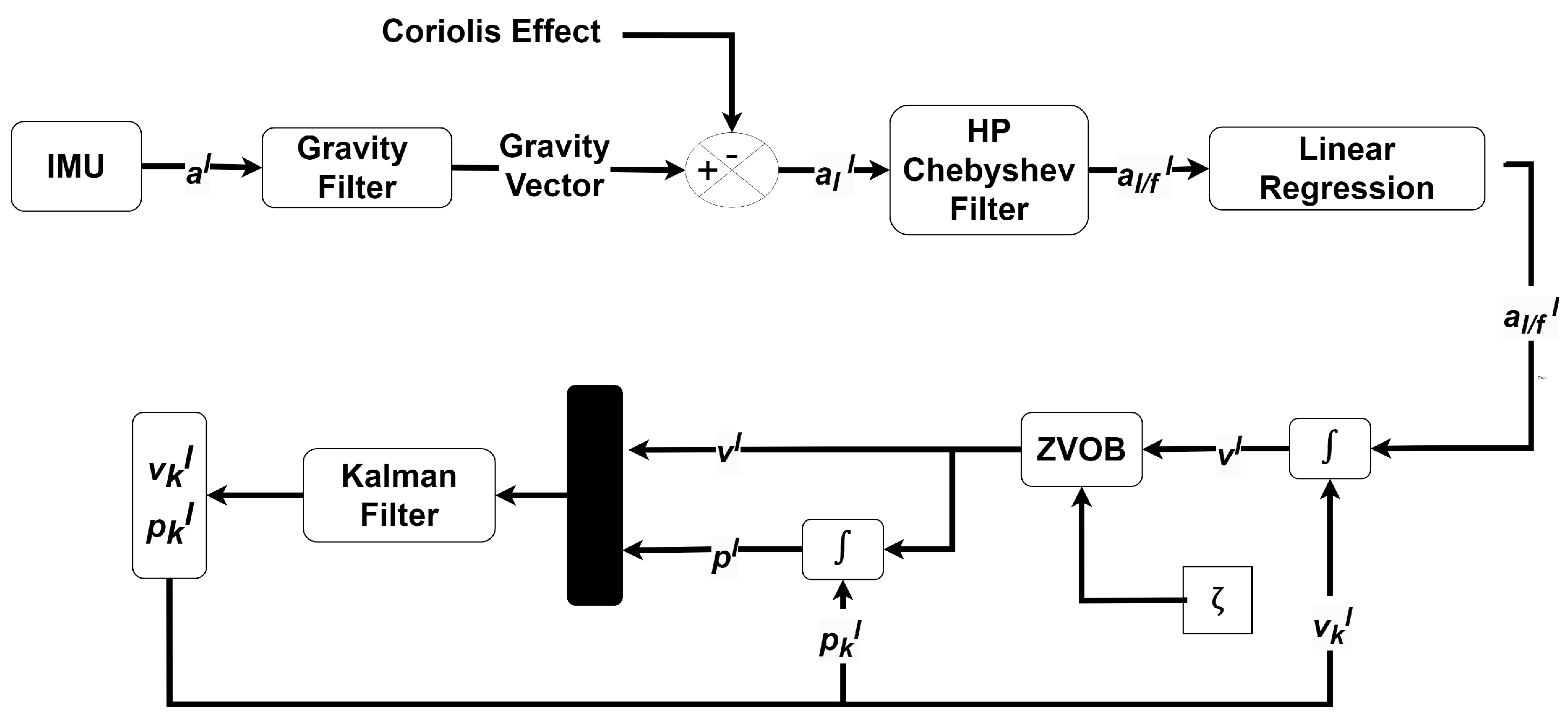
4. Inertial Displacement Monitoring System (IDMS) Methodology

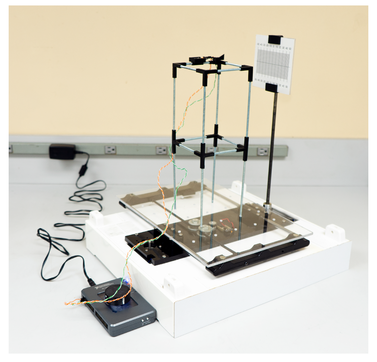
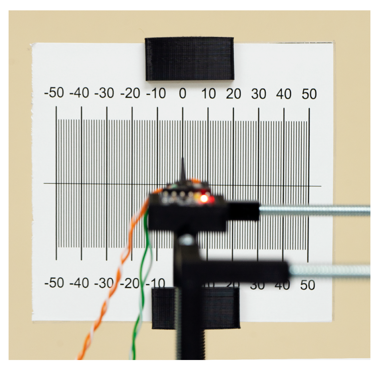
The IDMS is a methodology that implements an inertial system for monitoring the displacement in diverse structures under vibration. The system considers the inherent drift of inertial sensors. It also implements the correction algorithm ZVOB to calculate the position and measure the displacements when the structure is under movement, to diminish the vibrations caused by external factors. The correction algorithm works in conjunction with a Kalman filter and a Chebyshev filter to attenuate white noise and identify the oscillations in the structure; it also uses a Gravity filter for the inertial configuration ENU to avoid considering the gravity as a movement. In Figure 4, a block diagram with the IDMS methodology is shown.

The system initiates sample acquisition from the IMU’s accelerometer and gyroscope. First, the accelerometer data passes through the gravity filter to obtain the gravity vector as shown in Equation (11). Then, the inertial acceleration ${\mathit{a}}_I^l$ is calculated by implementing the sensor velocity ${\mathit{a}}^l$, which is 0 for an initial value, in conjunction with the information from the gyroscope, which includes the $\mathsf{\Omega }$ and ${\mathit{\omega }}^l$. As the system measures the displacement produced by seismic vibrations, it uses the accelerometer signal to determine the motion frequency, which requires proper signal conditioning. Hence, the data are filtered through a Chebyshev 6th-order filter to attenuate the low frequencies and preserve the information corresponding to the movements caused by the seismic vibrations. Afterward, a linear regression equation is calculated to estimate the frequency of the oscillation displacements. The equation implemented is shown in Equation (17) below, where $f_m$ is the frequency measured, $c_k$ are the linear regression coefficients and $Df$ is the dominant frequency.

$$Df\left(f_m\right)=c_1{f}_m^3+c_2{f}_m^2+c_3{f}_m+c_4$$

(17)

Afterwards, the acceleration ${\mathit{a}}_{I/f}^l$, is integrated to estimate ${\mathit{v}}^l$, which is the sensor-measured velocity. The information from ${\mathit{a}}_{I/f}^l$ and ${\mathit{v}}^l$ is used in the correction algorithm ZVOB in conjunction with the calculated tuning value $\mathit{\zeta }$ to define ${\mathit{v}}^l$ for the current iteration. Subsequently, the ${\mathit{v}}^l$ information is integrated to obtain ${\mathit{p}}^l$.

Therefore, the white noise in the calculated values ${\mathit{v}}_{n-1}^l$ and ${{\mathit{p}}^l}_{n-1}$ is attenuated through a Kalman filter. These values are considered as the past sample in the calculus of ${\mathit{v}}_n^l$ and ${{\mathit{p}}^l}_n$.

5. Experimentation

As mentioned, the IDMS measures the displacement of a structure under seismic conditions. Thus, to demonstrate the system’s capacity to measure displacement in seismic vibratory conditions, a shaking table was implemented that performed a seismic movement oscillating forwards and backward, simulating the wave motions of primary waves (P-wave). Furthermore, the shaking table performed the movements in one axis, and the IMU was aligned in that axis direction to measure the displacements. The experiment was performed on a shaking table that moved at defined frequencies:

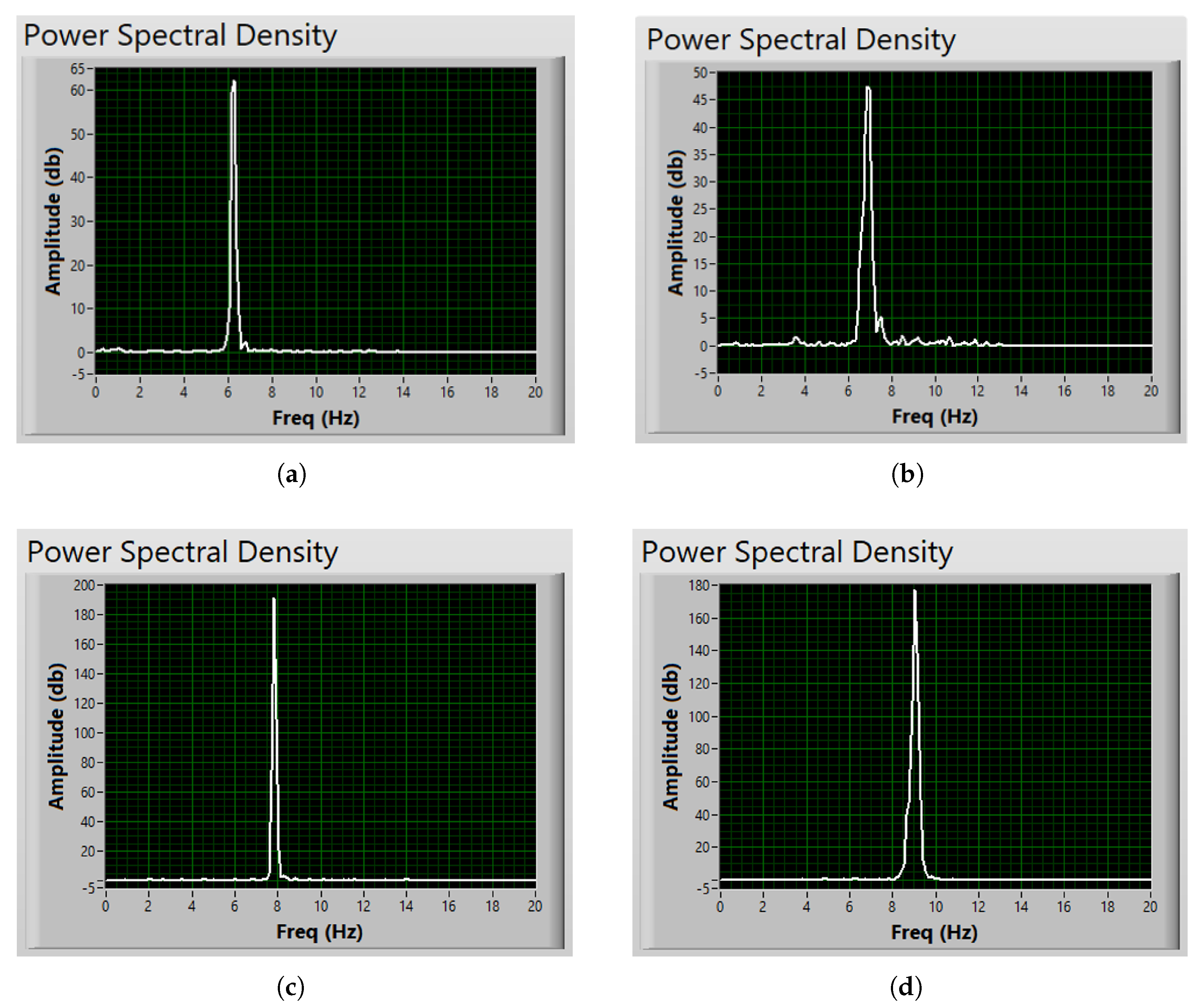
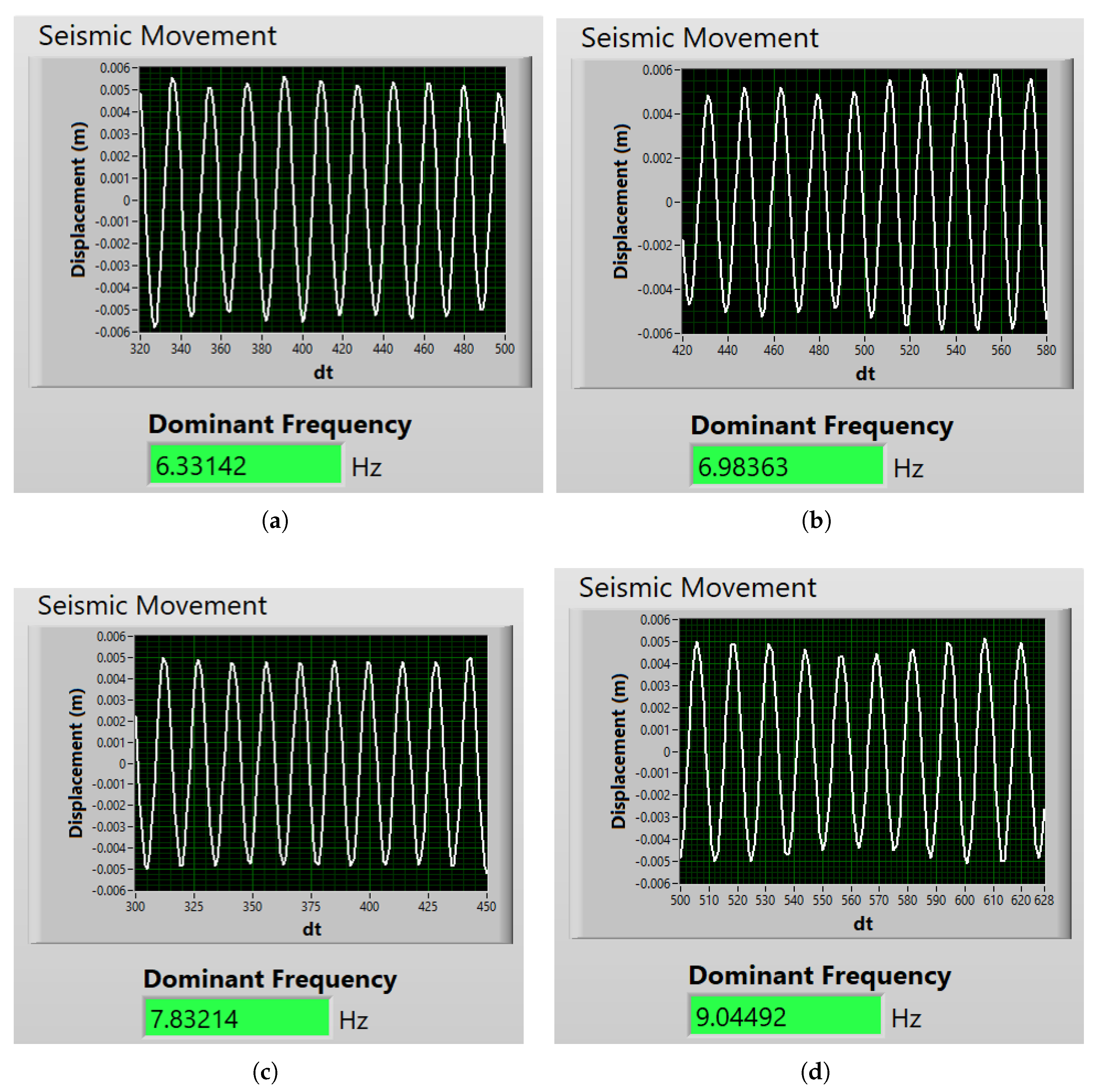
• 6.25 Hz movement in x-axis.
• 6.94 Hz movement in x-axis.
• 7.81 Hz movement in x-axis.
• 8.92 Hz movement in x-axis.

The selection of frequencies followed the range of the most common observed frequencies in seismic movements, and their average length time of 10 s was considered for the experiments [38,39,40]. The authors developed the shaking table; which includes such elements as fully threaded screws, a stepped motor 42HS4D-1704JA, and the PLA printed components of the structure used in the experiment; moreover, a program was created in Arduino, which runs on an ELEGOO UNO R3 controller board. The shaking table and the position of the IMU in the structure are shown in Figure 5.

The accelerometers were contained in an Invensense IMU MPU-9250 tracking device. The starting value in all the experiments was zero. The movement was performed over 5 s, and the other 5 s were in steady-state for comparison.

The inertial sensor movement at the top of the structure was measured with a graduated chart, as shown in Figure 6.

To ensure the accuracy of our results, we compared the measured movements with the actual displacement performed by the shaking table. This comparison was made possible by recording the movements with a high-quality slow-motion camera, with 12 MP, an aperture of f/1.6, and a 26 mm wide video setup of 1080p@120fps.

Therefore, experimentation data measured by the IMU (acceleration) were acquired with a MyRio of NI, an FPGA for data acquisition, and connected to an Asus TUF505 portable personal computer for processing and visualization. The sample rate of the captured read data was 1 ms. In the computer, a virtual instrument program was developed in order to implement the methodology and simultaneously take samples of data from the NIMyRio.

6. Results

The experiment results are presented in two phases: signal frequency analysis and displacement analysis. As different frequencies were employed in the experiment, verifying that the system was measuring at the same frequency at which the movements took place was required. Thus, the displacements calculated with the methodology were compared with the real displacements performed by the shaking table.

6.1. Signal Analysis

With the data obtained through the experiment, it was possible to compute the dominant frequency of the movements in each experiment realized. The IDMS identified a frequency accordant with the structure motion and posteriorly attenuated non-related frequencies resulting from the shaking table and other external sources [41,42]. In Figure 7, all the frequencies measured in the experimentation are presented; this includes the dominant frequency measured in every experiment and the external detected frequencies in the experimentation. As a Chebyshev filter was applied, the system only use the data at the mentioned frequency to calculate the displacements performed by the shaking table.

The data presented in

Table 1. Frequency analysis relative percentage error and RMSE.

Experiment Frequency (Hz)	System Frequency (Hz)	Relative Percentage Error
6.25	6.2546	1.33%
6.94	6.9527	1.74%
7.81	7.88367	0.49%
8.92	8.9375	1.004%
	Overall	1.14%
	RMSE	0.088

show the relative percentage error calculated in the frequency measured. Furthermore, the system frequency column shows the mean of all the experiment-measured frequencies for each of the four proposed experiment types. Finally, the last column displays the relative percentage error from all the experiments for each case. In the four experiments, a low relative percentage error existed in the measurement of the frequency and a “Root Mean Square Error” or “RMSE” of 0.088, which presents the system’s precision in determining the motion frequency at which the structure was performing the displacements. Therefore, the IDMS monitored the different excitations in the structure produced by seismic vibrations and attenuated those produced by the ambient elements. As a result, the system was capable of following the movements produced by the shaking table with precision, demonstrating that the displacements measured corresponded with the movements that occurred in the structure.

6.2. Displacement Measurements

As the IMDS calculated the frequency of the movements performed by the shaking table, the dominant frequency data were used to estimate and normalize the displacements. Posteriorly, the computed displacements were compared with the real displacements. In Figure 8, the four types of motion frequency performed by the shaking table are presented. Since the experiment simulated the seismic p-wave movement in a structure, the system measurement considered total displacement as the amplitude in a complete cycle.

It must be noted in

Table 2. Relative Percentage Error Analysis of the Measured Displacement.

Experiment Frequency (Hz)	Structure Displacement (mm)	System Measured Displacement (mm)	Relative Percentage Error
6.25	11.6000	11.8851	2.0132%
6.94	11.3000	11.6923	2.6201%
7.81	10.9000	11.6555	6.1587%
8.92	10.4000	10.4712	0.5712%
		RMSE	0.4092

that as the frequency of the oscillation increments, the total displacement diminishes. The reason for this is that the shaking table had to adapt to the selected movements, which reduced the displacement to perform the required oscillations for each experiment frequency.

In Table 2 is shown how the system followed the movement behavior with an RMSE of 0.4092, demonstrating the precision of most of the movements. Therefore, an increment in the relative percentage error of the frequency of 7.81 hz was noted. This was due to the difference in displacement between the experiment at frequencies of 6.25 and 6.94 in comparison with the other experiments.

Thus, in all four experiments, the IDMS presented a relative percentage error below 7%, demonstrating the system’s capacity to measure the displacement of structures under seismic motion. Additionally, as the system presented signal conditioning of the IMU’s accelerometer data to obtain a measurable distance in the x-axis, the drift presented in an inertial system is still a subject of interest for future works.

7. Discussion of the Results

The IDMS methodology is an inertial system that uses an IMU’s accelerometer to determine displacements when a structure is in motion due to seismic vibrations.

The experiments provided data to measure the motion frequency and measure the structural displacements when subjected to simulated p-wave seismic motion. Therefore, it was compared with other methodologies that also measure the displacement in structures under the influence of seismic motion.

In [43], a binocular vision system approach based on deep learning was proposed to measure a structure’s displacement. As the system measures tiny vibrations of a structure, performing image magnification of the motion is required, particularly where the displacement is smaller than one pixel.

However, ref. [44] presented a system for long-term monitoring, implementing four fiber-optic sensors to measure the structural displacements. This system considers the information of all the sensors in a structure; therefore, it is necessary to calibrate the current state of the structure’s components to prevent a reduction in the correlation between measurement of the sensors.

As a result, the mean errors in the displacement measurement of Shao’s and Garcia’s works were 9.02% and 4.44%, respectively, compared with the IDMS system, which presented a mean error of 2.84%. Additionally, the IDMS relies on the IMU’s accelerometer, which does not continuously re-evaluate the conditions of the structural components.

The work in [45] presented a multi-camera 3D DIC (digital image correlation) method using four high-speed cameras in a 1/8 scaled concrete structure. The multi-camera approach provides stereo vision measurements and the field of view cannot be overlapped. The RMSE in their x-axis displacement measurements was 0.43, compared to the IDMS’s RMSE of 0.409.

The system’s capacity to measure the displacement of structures demonstrates precision and efficiency under seismic vibratory conditions when monitoring the displacement produced in a structure.

8. Conclusions

The IDMS is an SHM methodology for performing continuous non-destructive measurements of a structure’s displacements when it is subjected to seismic motions. As with all inertial systems, the measurement signal of an accelerometer and a gyroscope contained in an IMU requires conditioning to correct the influence of drift and to properly predict the displacements of a structure under motion.

The conditioning phase involves Kalman and Chebyshev filters to reduce the influence of external perturbations and measure the motion frequency, to determine that the displacement measurement that corresponds to the seismic motion that the structure is subjected to. An algorithm called zero velocity observation update (ZVOB) was included to determine if a body is in motion or steady-state; this provides the system with adaptability to distinctive seismic movements and avoids the influence of external perturbations.

The IDMS methodology is designed to continuously monitor and measure displacements during seismic motion in a structure. The system was tested with experiments simulating seismic p-waves in one of the axes and aligning this with the accelerometers contained in the IMU, where the selection of the frequencies considered a range of typical frequencies of seismic movements in different parts of the world. Additionally, the time of the vibration motion in the experiments was performed according to the usual time length of seismic motions.

As a result, the IDMS measured frequencies with an RMSE of 0.088 hz overall, identifying the frequencies of the seismic vibrations and avoiding frequencies created by machines, human walking, or other external elements that could create errors in the measurement of the displacement. Furthermore, the system measured the displacement with an RMSE of 0.4092 mm, monitoring the different motions to which the structure was subjected.

Implementing the IDMS in different structures, such as multiple-floor buildings, bridges, or linear machines that are usually in a single line, could provides information to evaluate the structural conditions and prevent potential hazards due to structural failures. As the system monitors displacements, it is possible to detect separations in structural elements, the size of cracks, and delamination, or to elaborate studies to prevent structures from colliding with adjacent buildings.

The efficacy of the implemented ZVOB and analysis of the developed methodology demonstrated an inertial SHM system capable of measuring displacements under seismic vibratory conditions with precision. Furthermore, if the IDMS is implemented with multiple sensors at different points of the structure, adapting the current methodology could allow improving the precision, performing a better analysis to monitor displacements and vibration, and obtaining more data to complement the presented IDMS methodology.

For further research, multiple inertial sensors are being contemplated to build a nested IDMS and improve the obtained capabilities. Additionally, fusion with other technologies, such as laser scanning techniques, as mentioned by Castro-Toscano [46], could provide a wider range of measurements and detection of deformation in structures.

Additionally, it could be connected with other inertial sensors or with a network of similar sensors to improve measurement precision.

References

1. Zhang, C.; Mousavi, A.A.; Masri, S.F.; Gholipour, G.; Yan, K.; Li, X. Vibration feature extraction using signal processing techniques for structural health monitoring: A review. Mech. Syst. Signal Process. 2022, 177, 109175. [Google Scholar] [CrossRef]
2. Deng, Z.; Huang, M.; Wan, N.; Zhang, J. The Current Development of Structural Health Monitoring for Bridges: A Review. Buildings 2023, 13, 1360. [Google Scholar] [CrossRef]
3. Dang, H.V.; Tran-Ngoc, H.; Nguyen, T.V.; Bui-Tien, T.; De Roeck, G.; Nguyen, H.X. Data-Driven Structural Health Monitoring Using Feature Fusion and Hybrid Deep Learning. IEEE Trans. Autom. Sci. Eng. 2021, 18, 2087–2103. [Google Scholar] [CrossRef]
4. Shao, Y.; Li, L.; Li, J.; An, S.; Hao, H. Computer vision based target-free 3D vibration displacement measurement of structures. Eng. Struct. 2021, 246, 113040. [Google Scholar] [CrossRef]
5. Dong, C.Z.; Bas, S.; Catbas, F.N. Investigation of vibration serviceability of a footbridge using computer vision-based methods. Eng. Struct. 2020, 224, 111224. [Google Scholar] [CrossRef]
6. Zinno, R.; Haghshenas, S.S.; Guido, G.; VItale, A. Artificial Intelligence and Structural Health Monitoring of Bridges: A Review of the State-of-the-Art. IEEE Access 2022, 10, 88058–88078. [Google Scholar] [CrossRef]
7. Luan, L.; Zheng, J.; Wang, M.L.; Yang, Y.; Rizzo, P.; Sun, H. Extracting full-field subpixel structural displacements from videos via deep learning. J. Sound Vib. 2021, 505, 116142. [Google Scholar] [CrossRef]
8. Boscato, G.; Fragonara, L.Z.; Cecchi, A.; Reccia, E.; Baraldi, D. Structural Health Monitoring through Vibration-Based Approaches. Shock Vib. 2019, 2019, 2380616. [Google Scholar] [CrossRef]
9. Moradi, M.; Broer, A.; Chiachío, J.; Benedictus, R.; Loutas, T.H.; Zarouchas, D. Intelligent health indicator construction for prognostics of composite structures utilizing a semi-supervised deep neural network and SHM data. Eng. Appl. Artif. Intell. 2023, 117, 105502. [Google Scholar] [CrossRef]
10. Torzoni, M.; Manzoni, A.; Mariani, S. A Deep Neural Network, Multi-fidelity Surrogate Model Approach for Bayesian Model Updating in SHM. In European Workshop on Structural Health Monitoring; Rizzo, P., Milazzo, A., Eds.; Springer: Cham, Switzerland, 2023; pp. 1076–1086. [Google Scholar]
11. Lopez-Higuera, J.M.; Rodriguez Cobo, L.; Quintela Incera, A.; Cobo, A. Fiber Optic Sensors in Structural Health Monitoring. J. Light. Technol. 2011, 29, 587–608. [Google Scholar] [CrossRef]
12. Carani, L.B.; Martin, T.D.; Eze, V.O.; Okoli, O.I. Impact sensing and localization in composites structures with embedded mechanoluminescence-perovskite sensors. Sens. Actuators A Phys. 2022, 346, 113843. [Google Scholar] [CrossRef]
13. Rao, A.S.; Radanovic, M.; Liu, Y.; Hu, S.; Fang, Y.; Khoshelham, K.; Palaniswami, M.; Ngo, T. Real-time monitoring of construction sites: Sensors, methods, and applications. Autom. Constr. 2022, 136, 104099. [Google Scholar] [CrossRef]
14. Jeon, J.Y.; Miao, Y.; Park, G.; Flynn, E. Compressive laser scanning with full steady state wavefield for structural damage detection. Mech. Syst. Signal Process. 2022, 169, 108626. [Google Scholar] [CrossRef]
15. Choi, Y.; Abbas, S.H.; Lee, J.R. Aircraft integrated structural health monitoring using lasers, piezoelectricity, and fiber optics. Measurement 2018, 125, 294–302. [Google Scholar] [CrossRef]
16. Real-Moreno, O.; Rodríguez-Quiñonez, J.C.; Sergiyenko, O.; Flores-Fuentes, W.; Castro-Toscano, M.J.; Miranda-Vega, J.E.; Mercorelli, P.; Valdez-Rodríguez, J.A.; Trujillo-Hernández, G.; Sanchez-Castro, J.J. A Quadrant Approach of Camera Calibration Method for Depth Estimation Using a Stereo Vision System. In Proceedings of the IECON 2022—48th Annual Conference of the IEEE Industrial Electronics Society, Brussels, Belgium, 17–20 October 2022; pp. 1–6. [Google Scholar] [CrossRef]
17. Feng, D.; Feng, M.Q. Identification of structural stiffness and excitation forces in time domain using noncontact vision-based displacement measurement. J. Sound Vib. 2017, 406, 15–28. [Google Scholar] [CrossRef]
18. Trujillo-Hernández, G.; Rodríguez-Quiñonez, J.C.; Flores-Fuentes, W.; Sergiyenko, O.; Ontiveros-Reyes, E.; Real-Moreno, O.; Hernández-Balbuena, D.; Murrieta-Rico, F.N.; Rascón, R. Development of an integrated podometry system for mechanical load measurement and visual inspection. Measurement 2022, 203, 111866. [Google Scholar] [CrossRef]
19. Veluthedath Shajihan, S.A.; Chow, R.; Mechitov, K.; Fu, Y.; Hoang, T.; Spencer, B.F. Development of Synchronized High-Sensitivity Wireless Accelerometer for Structural Health Monitoring. Sensors 2020, 20, 4169. [Google Scholar] [CrossRef] [PubMed]
20. Shih, J.Y.; Weston, P.; Entezami, M.; Roberts, C.; O’Callaghan, M. Experiences Using MEMS Accelerometers on Railway Bearers at Switches and Crossings to Obtain Displacement—Awkward Situations. Infrastructures 2024, 9, 91. [Google Scholar] [CrossRef]
21. Hassani, S.; Dackermann, U.; Mousavi, M.; Li, J. A systematic review of data fusion techniques for optimized structural health monitoring. Inf. Fusion 2024, 103, 102136. [Google Scholar] [CrossRef]
22. Qu, X.; Ding, X.; Xu, Y.L.; Yu, W. Real-time outlier detection in integrated GNSS and accelerometer structural health monitoring systems based on a robust multi-rate Kalman filter. J. Geod. 2023, 97, 38. [Google Scholar] [CrossRef]
23. Castro-Toscano, M.; Rodríguez-Quiñonez, J.; Hernández-Balbuena, D.; Rivas-Lopez, M.; Sergiyenko, O.; Flores-Fuentes, W. Obtención de Trayectorias Empleando el Marco Strapdown INS/KF: Propuesta Metodológica. Rev. Iberoam. Autom. Inform. Ind. 2018, 15, 391–403. [Google Scholar] [CrossRef]
24. Rodríguez-Quiñonez, J.C. Intelligent Automatic Object Tracking Method by Integration of Laser Scanner System and INS. Program. Comput. Softw. 2020, 46, 619–625. [Google Scholar] [CrossRef]
25. Castro-Toscano, M.J.; Valdez-Rodríguez, J.A.; Rodríguez-Quiñonez, J.C.; Flores-Fuentes, W.; Sergiyenko, O.; Trujillo-Hernandez, G.; Real-Moreno, O. Determination of Trajectories Using IKZ/CF Inertial Navigation: Methodological Proposal/CF Inertial Navigation: Methodological Proposal. Heliyon 2023, 9, e13863. [Google Scholar] [CrossRef] [PubMed]
26. Sokolov, S.; Pogorelov, V.; Shatalov, A. Solving the Autonomous Initial Navigation Task for Strapdown Inertial Navigation System on the Perturbed Basis Using Rodriguez—Hamilton Parameters. Russ. Aeronaut. 2019, 62, 42–51. [Google Scholar] [CrossRef]
27. Bose, A.; Bhat, K.; Kurian, T. Fundamentals of Navigation and Inertial Sensors; Eastern Economy Edition; PHI Learning: Delhi, India, 2014. [Google Scholar]
28. Valdez-Rodríguez, J.A.; Rodríguez-Quiñonez, J.C.; Flores-Fuentes, W.; Ramírez-Hernández, L.R.; Trujillo-Hernández, G.; Real-Moreno, O.; Castro-Toscano, M.J.; Miranda-Vega, J.E.; Mercorelli, P. Visual-Inertial Navigation Systems and Technologies. In Optoelectronic Devices in Robotic Systems; Sergiyenko, O., Ed.; Springer International Publishing: Cham, Switzerland, 2022; pp. 137–166. [Google Scholar] [CrossRef]
29. Lin, Y.; Zhang, W.; Xiong, J. Specific force integration algorithm with high accuracy for strapdown inertial navigation system. Aerosp. Sci. Technol. 2015, 42, 25–30. [Google Scholar] [CrossRef]
30. Acar, C.; Shkel, A. Introduction; MEMS Vibratory Gyroscopes: Structural Approaches to Improve Robustness. In MEMS Vibratory Gyroscopes: Structural Approaches to Improve Robustness; Springer US: Boston, MA, USA, 2009; pp. 1–14. [Google Scholar] [CrossRef]
31. Klančar, G.; Zdešar, A.; Blažič, S.; Škrjanc, I. Chapter 5—Sensors Used in Mobile Systems. In Wheeled Mobile Robotics; Klančar, G., Zdešar, A., Blažič, S., Škrjanc, I., Eds.; Butterworth-Heinemann: Oxford, UK, 2017; pp. 207–288. [Google Scholar] [CrossRef]
32. Kumari, N.; Kulkarni, R.; Ahmed, M.R.; Kumar, N. Use of Kalman Filter and Its Variants in State Estimation: A Review. In Artificial Intelligence for a Sustainable Industry 4.0; Awasthi, S., Travieso-González, C.M., Sanyal, G., Kumar Singh, D., Eds.; Springer International Publishing: Cham, Switzerland, 2021; pp. 213–230. [Google Scholar] [CrossRef]
33. Quan, W.; Gong, X.; Fang, J.; Li, J. INS/GNSS Integrated Navigation Method. In INS/CNS/GNSS Integrated Navigation Technology; Springer Berlin Heidelberg: Berlin/Heidelberg, Germany, 2015; pp. 185–235. [Google Scholar] [CrossRef]
34. Wang, Y.; Shkel, A.M. Adaptive Threshold for Zero-Velocity Detector in ZUPT-Aided Pedestrian Inertial Navigation. IEEE Sens. Lett. 2019, 3, 1–4. [Google Scholar] [CrossRef]
35. Tong, X.; Su, Y.; Li, Z.; Si, C.; Han, G.; Ning, J.; Yang, F. A Double-Step Unscented Kalman Filter and HMM-Based Zero-Velocity Update for Pedestrian Dead Reckoning Using MEMS Sensors. IEEE Trans. Ind. Electron. 2020, 67, 581–591. [Google Scholar] [CrossRef]
36. Benzerrouk, H.; Nebylov, A.V. Robust IMU/UWB integration for indoor pedestrian navigation. In Proceedings of the 2018 25th Saint Petersburg International Conference on Integrated Navigation Systems (ICINS), Saint Petersburg, Russia, 28–30 May 2018; pp. 1–5. [Google Scholar] [CrossRef]
37. Suresh, R.P.; Sridhar, V.; Pramod, J.; Talasila, V. Zero Velocity Potential Update (ZUPT) as a Correction Technique. In Proceedings of the 2018 3rd International Conference On Internet of Things: Smart Innovation and Usages (IoT-SIU), Bhimtal, India, 23–24 February 2018; pp. 1–8. [Google Scholar] [CrossRef]
38. Schwardt, M.; Pilger, C.; Gaebler, P.; Hupe, P.; Ceranna, L. Natural and Anthropogenic Sources of Seismic, Hydroacoustic, and Infrasonic Waves: Waveforms and Spectral Characteristics (and Their Applicability for Sensor Calibration). Surv. Geophys. 2022, 43, 1265–1361. [Google Scholar] [CrossRef] [PubMed]
39. Aydan, Ö. Earthquake Science and Engineering; CRC Press: London, UK, 2022. [Google Scholar]
40. Towhata, I. Geotechnical Earthquake Engineering; Springer Series in Geomechanics and Geoengineering; Springer: Berlin/Heidelberg, Germany, 2008. [Google Scholar]
41. Chen, Y.; Li, H.; Hou, L.; Bu, X. Feature extraction using dominant frequency bands and time-frequency image analysis for chatter detection in milling. Precis. Eng. 2019, 56, 235–245. [Google Scholar] [CrossRef]
42. Shi, Y.; Mahr, F.; von Wagner, U.; Uhlmann, E. Chatter frequencies of micromilling processes: Influencing factors and online detection via piezoactuators. Int. J. Mach. Tools Manuf. 2012, 56, 10–16. [Google Scholar] [CrossRef]
43. Shao, Y.; Li, L.; Li, J.; An, S.; Hao, H. Target-free 3D tiny structural vibration measurement based on deep learning and motion magnification. J. Sound Vib. 2022, 538, 117244. [Google Scholar] [CrossRef]
44. Garcia-Sanchez, D.; Fernandez-Navamuel, A.; Sánchez, D.Z.; Alvear, D.; Pardo, D. Bearing assessment tool for longitudinal bridge performance. J. Civ. Struct. Health Monit. 2020, 10, 1023–1036. [Google Scholar] [CrossRef]
45. Wei, K.; Yuan, F.; Shao, X.; Chen, Z.; Wu, G.; He, X. High-speed multi-camera 3D DIC measurement of the deformation of cassette structure with large shaking table. Mech. Syst. Signal Process. 2022, 177, 109273. [Google Scholar] [CrossRef]
46. Castro-Toscano, M.J.; Rodríguez-Quiñonez, J.C.; Sergiyenko, O.; Flores-Fuentes, W.; Ramirez-Hernandez, L.R.; Hernández-Balbuena, D.; Lindner, L.; Rascón, R. Novel sensing approaches for structural deformation monitoring and 3D measurements. IEEE Sens. J. 2020, 21, 11318–11328. [Google Scholar] [CrossRef]
Figure 1. IDMS: A SHM system for the measurement of displacements through an inertial system methodology.
Infrastructures 09 00116 g001
Figure 2. The IMU position in one of the links at the top of the structure to measure the displacements realized.
Infrastructures 09 00116 g002
Figure 3. ZVOB flowchart.
Infrastructures 09 00116 g003
Figure 4. IDMS methodology: the block diagram shows the structure of the system. Monitoring is performed implementing the correction algorithm ZVOB, the filters of Kalman, Chebyshev, and Gravity, complemented by inertial equations to calculate the displacement of a structure.
Infrastructures 09 00116 g004
Figure 5. Shaking table and IMU position for the experiments.
Infrastructures 09 00116 g005
Figure 6. The inertial sensor movement was measured with a graduated chart in millimeters. In order to verify the precision of the displacement, the movements were recorded with a slow-motion camera.
Infrastructures 09 00116 g006
Figure 7. Power Spectral density chart showing the dominant frequency in each of the experiments. The graphics present the dominant frequency of the oscillation movements. (a) Frequency measured for a seismic vibratory movement that oscillated at 6.25 Hz. (b) Frequency measured for a seismic vibratory movement that oscillated at 6.94 Hz. (c) Frequency measured for a seismic vibratory movement that oscillated at 7.81 Hz. (d) Frequency measured for a seismic vibratory movement that oscillated at 8.92 Hz.
Infrastructures 09 00116 g007
Figure 8. Total displacements and measured frequency. (a) Total displacement and frequency measured for the movement at 6.25 Hz. (b) Total displacement and frequency measured for the movement at 6.94 Hz. (c) Total displacement and frequency measured for the movement at 7.81 Hz. (d) Total displacement and frequency measured for the movement at 8.92 Hz.
Infrastructures 09 00116 g008