A Comparative Study of YOLO, SSD, Faster R-CNN, and More for Optimized Eye-Gaze Writing

Abstract

Eye-gaze writing technology holds significant promise but faces several limitations. Existing eye-gaze-based systems often suffer from slow performance, particularly under challenging conditions such as low-light environments, user fatigue, or excessive head movement and blinking. These factors negatively impact the accuracy and reliability of eye-tracking technology, limiting the user’s ability to control the cursor or make selections. To address these challenges and enhance accessibility, we created a comprehensive dataset by integrating multiple publicly available datasets, including the Eyes Dataset, Dataset-Pupil, Pupil Detection Computer Vision Project, Pupils Computer Vision Project, and MPIIGaze dataset. This combined dataset provides diverse training data for eye images under various conditions, including open and closed eyes and diverse lighting environments. Using this dataset, we evaluated the performance of several computer vision algorithms across three key areas. For object detection, we implemented YOLOv8, SSD, and Faster R-CNN. For image segmentation, we employed DeepLab and U-Net. Finally, for self-supervised learning, we utilized the SimCLR algorithm. Our results indicate that the Haar classifier achieves the highest accuracy (0.85) with a model size of 97.358 KB, while YOLOv8 demonstrates competitive accuracy (0.83) alongside an exceptional processing speed and the smallest model size (6.083 KB), making it particularly suitable for cost-effective real-time eye-gaze applications.

1. Introduction

Eye-gaze writing is a novel interaction modality with the potential to revolutionize communication for individuals with limited mobility [1]. However, this technology faces several limitations. In low-light conditions or when users experience eye fatigue or irritation, excessive head movement or blinking can hinder eye-tracking accuracy, making it difficult to control the cursor or select items. Additionally, eye-gaze writing tends to be slower than traditional keyboard typing, particularly for new users or individuals with limited eye control. Prolonged use of eye-gaze writing and blinking can also lead to eye strain, further affecting accuracy and speed. Moreover, certain medical conditions, such as amblyopia or strabismus, can make eye-gaze writing more challenging for some users.

We developed our dataset by integrating multiple online available datasets, each offering unique advantages. By combining these datasets, we aimed to create a diverse collection of eye images, ensuring robustness in challenging conditions such as eye fatigue, irritation, and low lighting.

We investigate three key areas in computer vision: object detection, image segmentation, and self-supervised learning. Object detection algorithms are employed to identify and localize objects within an image. In our case, they are used to determine the user’s gaze direction by accurately detecting the pupil and iris positions. Image segmentation techniques are utilized to isolate the eye region from the rest of the image, improving object detection precision and reducing noise. This approach is particularly beneficial when the user is wearing glasses or experiencing eye fatigue. Lastly, self-supervised learning is leveraged to pre-train deep learning models on large unlabeled datasets, enhancing the accuracy, speed, and robustness of eye-gaze recognition and text input by identifying the most effective algorithms.

We aim to evaluate the system’s user-friendliness, ease of use, and speed. Additionally, we seek to identify the algorithm that achieves the best performance in terms of both speed and accuracy, selecting it for further development. Therefore, we asked different people to test our models. One user was wearing glasses that reflected the light so we could test image semantic segmentation in our iris’s small size.

To reduce the fatigue caused by prolonged blinking, we designed our models to register a letter selection after the user maintains focus on it for a few seconds, eliminating the need for blinking as an input method. Our contributions are the following:

• Applying computer vision and machine learning models to increase the speed of the eye-gaze writing: We evaluate the efficiency of deep learning algorithms for real-time eye-gaze writing, aiming to enhance both speed and accuracy. Specifically, we assess three object detection models —- YoLOv8, SSD, and Faster R-CNN- to address the challenge of detecting the small iris with high precision. For image segmentation, we employ DeepLab and U-Net to improve robustness in scenarios where users wear glasses or makeup or have eye conditions such as amblyopia or strabismus. Additionally, we explore SimCLR for self-supervised learning to enhance feature representation without requiring extensive labeled data.
• Overcome the limitations of eye-gaze writing: Eye-tracking technology struggles in low light conditions or when users experience eye fatigue, irritation, excessive head motion, or blinking, affecting accuracy [2]. To address these challenges, we create a new dataset by combining multiple datasets, providing diverse training data for various eye states and lighting conditions.
• Overcome fatigue caused by blinking: To overcome fatigue caused by blinking for a significant amount of time, we design our models to focus on a letter for seconds so that the letter will be written and cancel blinking.

2. Related Work

In the early 20th century, pioneering researchers such as J. W. Baird and L. T. Clark introduced the concept of using eye movements as an input modality instead of relying on hand-based interaction. Significant advancements in eye-tracking technology during the mid-20th century laid the foundation for practical eye-gaze writing systems. However, early systems were often bulky and lacked accuracy, limiting their usability. Modern technological advancements have addressed these challenges, resulting in more precise, reliable, and cost-effective eye-gaze tracking systems. The following sections provide an in-depth exploration of these technologies.

2.1. Pupil Center Corneal Reflection Technique (PCCR)

The working principle of Pupil Center Corneal Reflection (PCCR) can be compared to a tiny flashlight emitting a beam into the eye. The reflection of this light accurately tracks the user’s gaze position. This method is affordable, but systems based on PCCR algorithms suffer from two main limitations: the calibration [3] must be performed multiple times for each individual, and the system has a low tolerance for head movements, requiring the user to hold their head uncomfortably still. These two disadvantages hinder the widespread adoption of this algorithm, and numerous studies [4] have been published attempting to enhance its performance and overcome these limitations.

2.2. Appearance-Based Methods

Appearance-based methods analyze the overall appearance of the eye region in images or video frames to estimate gaze direction. They track the eye-gaze direction by analyzing the eyes, such as the pupil size and the patterns in the iris. Studies [5] demonstrated the potential of this approach for eye-gaze writing (EGW). However, they also highlighted challenges related to the diversity of eye colors and shapes among individuals, which can affect performance. Another limitation is that significant changes in lighting or obstructions, such as sunglasses or makeup, can impact the system’s performance, potentially leading to reduced accuracy. To enhance the appearance-based methods, the researchers constructed the MPIIGaze dataset [6], which contains images capturing diverse gaze directions and head poses in realistic environments. The researchers [7] used CNNs like AlexNet and VGG for feature extraction in appearance-based gaze tracking.

2.3. Saccadic and Fixational Analysis

Saccadic and Fixational Analysis tracks eye-gaze movements, including rapid flicks (saccades) and brief pauses (fixations) [8]. By analyzing these patterns, the system can infer which letter the user is focusing on and select it accordingly. However, a key limitation of this approach is that involuntary eye twitches or independent eye movements may be misinterpreted as intentional selections. Ongoing research seeks to refine these methods to better distinguish between deliberate glances at a letter and unintentional eye movements.

2.4. Model-Based Methods

Model-based methods estimate gaze direction using geometric and mathematical models of the eye. These approaches rely on key eye landmarks such as the pupil center, corneal reflection (PCCR), and overall eye geometry. Model-based methods offer advantages like greater interpretability and reduced data requirements. However, they are sensitive to lighting conditions, head movements, and individual eye variations. Studies [9] demonstrated their effectiveness for eye gaze writing (EGW) but also highlighted the need for sufficient computational power to achieve smooth real-time performance [10].

2.5. The Haar Cascade Classifier

Haar, as shown in Figure 1, was first introduced by Viola and Jones in 2001 [11,12].

The rectangular Haar features [13] are black and white rectangle patterns used to measure the contrast between different regions of an image. In eye detection, Haar features identify the eye region by scanning the face, detecting patterns such as the dark iris contrasting against the lighter sclera. We developed our code and models to integrate with the Haar Cascade Classifier, utilizing it for iris detection because of its effectiveness in identifying the eye region. Additionally, we employed OpenCV with a pre-trained Haar model for eye detection. Our contributions begin after detecting the eye region, where we apply our models.

Table 1. Comparative study.

Technique	Accuracy	Low Light	Speed
Saccadic and Fixational	High	Low	Medium
Model-based	High	Medium	Low
Appearance-based	Medium	Low	Slow
PCCR technique	High	Medium	Slow
Haar Cascade Classifier	High	Medium	Fast
YOLOv8 (our model)	High	High	Fast
SSD (our model)	High	High	Fast

presents a comparison between the proposed models and the models previously employed.

3. Methodology

3.1. Workflow Overview

We designed our system by evaluating key areas of computer vision, including YOLOv8, SSD, Faster R-CNN, DeepLab, U-Net, and SimCLR, to enhance both the speed and accuracy of eye-gaze writing (EGW). Our models were trained on a diverse dataset created by integrating multiple publicly available datasets, each offering unique advantages. This comprehensive dataset ensures robustness in various conditions, such as eye fatigue, irritation, and low-light environments. Through this comparative analysis, we identify the most efficient model for real-time eye-gaze writing applications.

3.2. Datasets and Data Preprocessing

We initially utilized the MPIIGaze dataset [14], which contains 213,659 images captured under diverse conditions. However, it did not yield the expected results. After multiple trials, we constructed a comprehensive dataset by integrating various sources, each offering unique advantages. The Eyes Dataset [15] (857 images) distinguishes between “Eyes OPEN” and “Eyes CLOSE”. The Dataset-Pupil [16] (308 images) includes images under purple lighting, with and without glasses. The Pupil Detection Computer Vision Project [17] (5193 images) and the Pupils Computer Vision Project [18] (1344 images) provide diverse lighting conditions, different eye colors, and variations such as makeup, ensuring robustness for pupil detection.

Figure 2 presents the data preprocessing and augmentation pipeline for integrating multiple eye-gaze datasets. Preprocessing ensured consistency by resizing all images to 640 × 640 pixels and applying auto-orientation for pixel alignment. To reduce biases and enhance model robustness, dataset-specific augmentation techniques were employed.

• Eyes Dataset and Dataset-Pupil: applied Gaussian blur (kernel size: 0–1.25 pixels) to reduce noise and brightness adjustments (−25% to +25%) to simulate varying lighting conditions.
• Pupil Detection Computer Vision Project: introduced diverse augmentations, including brightness adjustments (−5% to +5%), cropping (0−5%) for occlusion handling, rotations (−10° to +10°) for camera angle variations, and exposure adjustments (−3% to +3%).
• Pupils Computer Vision Project: converted images to grayscale to remove color dependency, supplemented by Gaussian blur and brightness adjustments to enhance generalization.

Figure 2. How we combined the datasets to obtain our dataset.

Figure 2. How we combined the datasets to obtain our dataset.

The augmented and preprocessed data from all sources were integrated into a unified dataset, “Our Data” comprising 221,361 eye images captured under diverse lighting conditions, with and without makeup and glasses. This integration, combined with tailored augmentation strategies, mitigates overfitting risks related to specific lighting, eye types, or camera angles, thereby improving the model’s generalization to real-world scenarios.

3.3. Proposed Gaze Prediction Models

We selected YOLOv8, SSD, Faster R-CNN, DeepLabv3, U-Net, and SimCLR for their diverse architectures and suitability for gaze and pupil detection. Each model brings distinct advantages, addressing different aspects of the task.

3.4. Model Selection

We selected the following models for their suitability in gaze and pupil detection:

• YOLOv8: Balances speed and accuracy, making it ideal for real-time applications.
• SSD: efficiently detects objects in a single forward pass, reducing computational cost.
• Faster R-CNN: achieves high detection accuracy, particularly for small objects like pupils, though with longer inference times.
• DeepLabv3: excels in semantic segmentation, improving precise boundary detection of the pupil.
• U-Net: well suited for detailed segmentation tasks, commonly used in medical imaging.
• SimCLR: Enhances feature extraction using contrastive learning, beneficial when labeled data are limited.

We did not include alternative architectures, such as EfficientDet and DETR, due to computational constraints and their compatibility with the existing experimental setup.

3.4.1. YOLO: You Only Look Once

YOLOv8, as shown in Figure 3, released by Ultralytics on 10 January 2023, is a state-of-the-art model that enhances detection accuracy and speed compared to its predecessors in the YOLO series. Its architecture comprises three primary components: the backbone, neck, and head [19].

The model adopts CSPDarknet53 [20] as its backbone, where input features are progressively down-sampled across five scales (A1 to A5) to extract multi-scale features. To improve performance, the CSP module was replaced with the C2f module, which enriches information flow through gradient shunt connections while maintaining a lightweight design. Additionally, the CBS module applies convolution followed by batch normalization and SiLU activation, while the Spatial Pyramid Pooling Fast (SPPF) module [21] pools input feature maps into fixed sizes, enhancing adaptability.

For the neck, YOLOv8 utilizes the PAN-FPN system [22], which enhances feature diversity by integrating the Path Aggregation Network (PAN) into the Feature Pyramid Network (FPN). This dual-direction structure facilitates deeper semantic learning through top-down pathways while retaining positional information via bottom-up pathways, merging scales A6–A7 and B1–B2 to improve feature fusion and completeness. Notably, YOLOv8 omits the convolution operation after up-sampling in PAN, ensuring a lighter model without compromising performance.

The head structure features a decoupled design, allocating separate components for object classification and localization, with binary cross-entropy loss (BCE loss) applied for classification, and distribution focal loss (DFL) [23] and Complete Intersection over Union (CIoU) [24] used for bounding box regression. As an anchor-free model, YOLOv8 dynamically assigns samples during training through the Task-Aligned Assigner [25], enhancing detection accuracy and robustness.

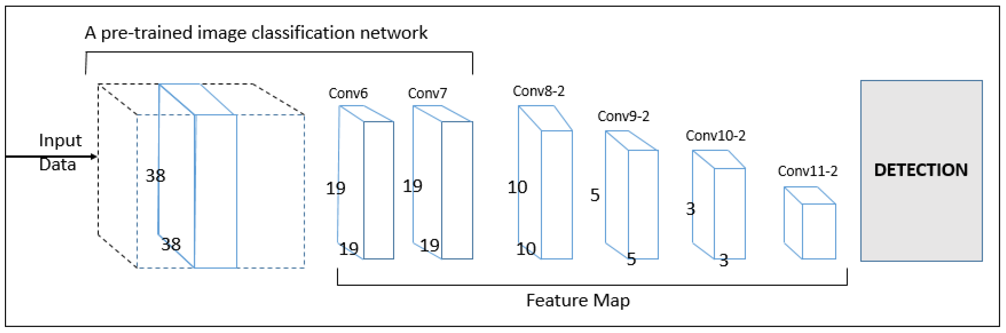
3.4.2. SSD: Single Shot Multi-Box Detector

SSD stands for Single Shot Multi-Box Detector. SSD is known for its speed and efficiency. It was first introduced in [26] in 2016.

SSD comprises two main components, as shown in Figure 4: the backbone model and the SSD head [27]. The backbone model typically serves as a feature extractor and is often a pre-trained image classification network, such as AlexNet, ResNet, or VGG [28], with the final fully connected classification layer removed. The SSD head, on the other hand, consists of one or more convolutional layers responsible for detecting objects at various scales. Training an SSD model from scratch requires a large dataset. Therefore, in this study, we imported pre-trained weights from the Caffe Face Detector Model [29] using OpenCV. The model’s outputs are interpreted as bounding boxes and object classes derived from the spatial locations of the final layer’s activations.

3.4.3. Faster R-CNN: Faster Region-Based Convolutional Neural Network

Faster R-CNN, an advancement of the R-CNN architecture [30], enhances object detection by integrating Region Proposal Networks (RPNs) with convolutional neural networks (CNNs), streamlining the detection pipeline and improving efficiency [31].

Figure 5 shows how the R-CNN family operates by generating region proposals to identify potential object locations, extracting key features using CNNs, predicting object classes through classification, and refining bounding box coordinates via regression. Compared to its predecessors, Faster R-CNN leverages deep-learning-based region proposal generation rather than CPU-based algorithms, reducing proposal time per image from 2 s to 10 ms while achieving greater accuracy [32].

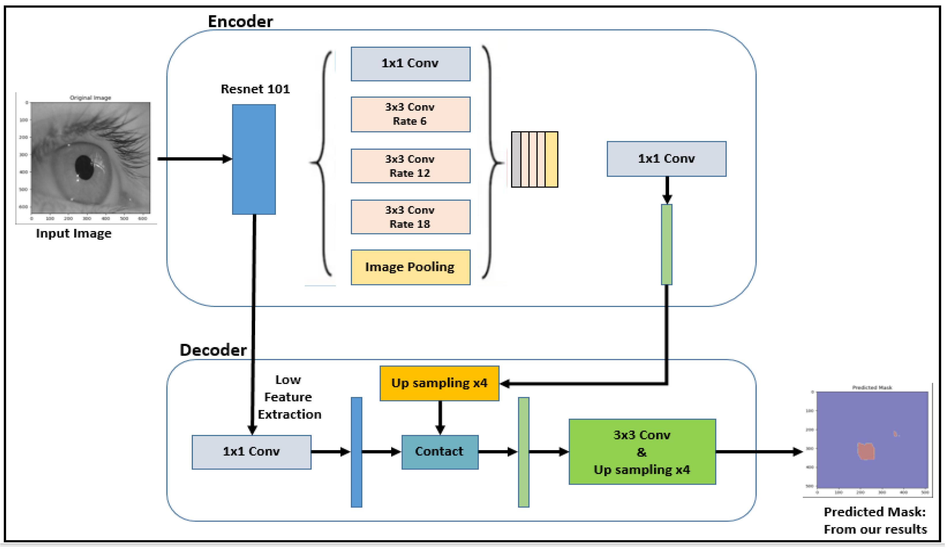
3.4.4. DeepLab: Deep Convolutional Neural Networks

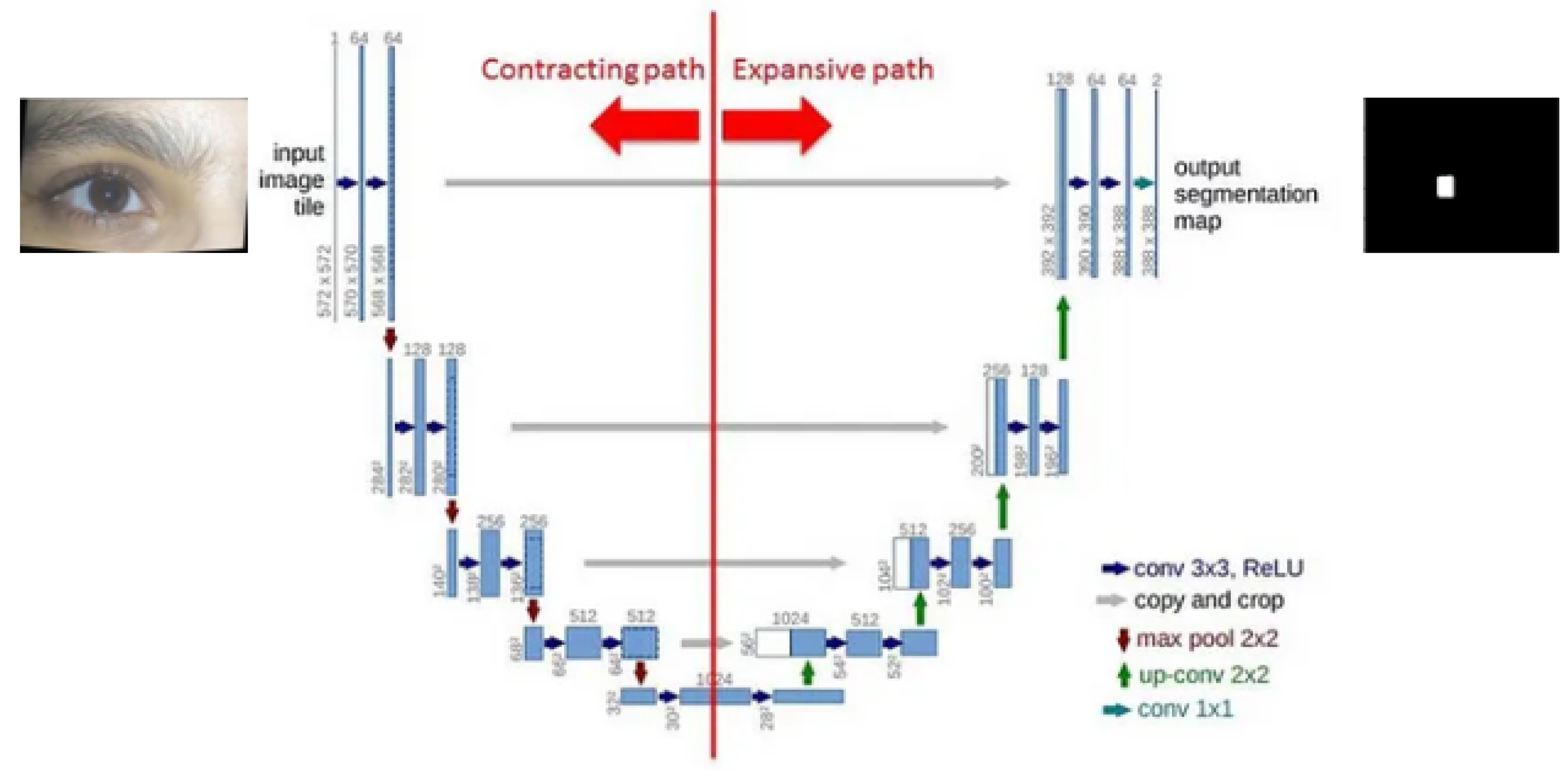
Deep convolutional neural networks (DCNNs) are renowned for their ability to extract rich feature representations, making them highly effective in object localization, detection, and image segmentation tasks. In this study, DeepLabv3 was selected due to its advanced segmentation performance. Figure 6 shows that the architecture consists of two primary components: the encoder and the decoder, each crucial for accurately segmenting the iris region.

The encoder employs ResNet-101 as its backbone, assigning pixel-wise classifications to identify the eye iris [33]. It utilizes atrous convolutions with different dilation rates (6, 12, and 18) to capture features at multiple scales, while an image pooling step aggregates global contextual information. A 1 × 1 convolution is then applied to refine these combined features, enhancing the model’s capacity for precise iris delineation.

The decoder integrates low-level features from earlier layers to retain fine-grained details essential for accurate segmentation. It up-samples the encoded features by a factor of four to match the original image dimensions and concatenates them with the low-level features to improve accuracy. Finally, a 3 × 3 convolution and another fourfold up-sampling produce the final mask, effectively highlighting the iris region.

3.4.5. U-Net

U-Net is a convolutional neural network architecture specifically designed for image segmentation tasks. Its distinctive U-shaped structure enables the network to capture both contextual information and fine-grained image details, making it highly effective for segmentation [34]. The architecture consists of two primary paths: the contracting path and the expansive path, as shown in Figure 7.

The contracting path employs a series of two 3 × 3 convolutions [35], each followed by a Rectified Linear Unit (ReLU) activation function [36], and a 2 × 2 max-pooling operation [37] with a stride of 2 for down-sampling. This process reduces the spatial dimensions while increasing the number of feature channels, thereby enhancing the network’s capacity to learn complex patterns. At each down-sampling step, the number of features is doubled, progressively capturing high-level features while compressing the data representation [38].

The expansive path focuses on up-sampling the feature maps to restore the original spatial resolution. Each stage begins with a 2 × 2 transposed convolution, doubling the spatial dimensions while halving the number of feature channels. The up-sampled feature maps are concatenated with the corresponding feature maps from the contracting path, ensuring the preservation of both high-level contextual information and fine-grained spatial details. Subsequently, two 3 × 3 convolutions, each followed by a ReLU activation function, refine the feature representations. Due to pixel loss at the borders during convolution, cropping is performed to align the feature maps before concatenation. Finally, a 1 × 1 convolution layer produces the desired number of output classes. In total, U-Net comprises 23 convolutional layers, enabling it to effectively learn and reconstruct complex features for precise image segmentation.

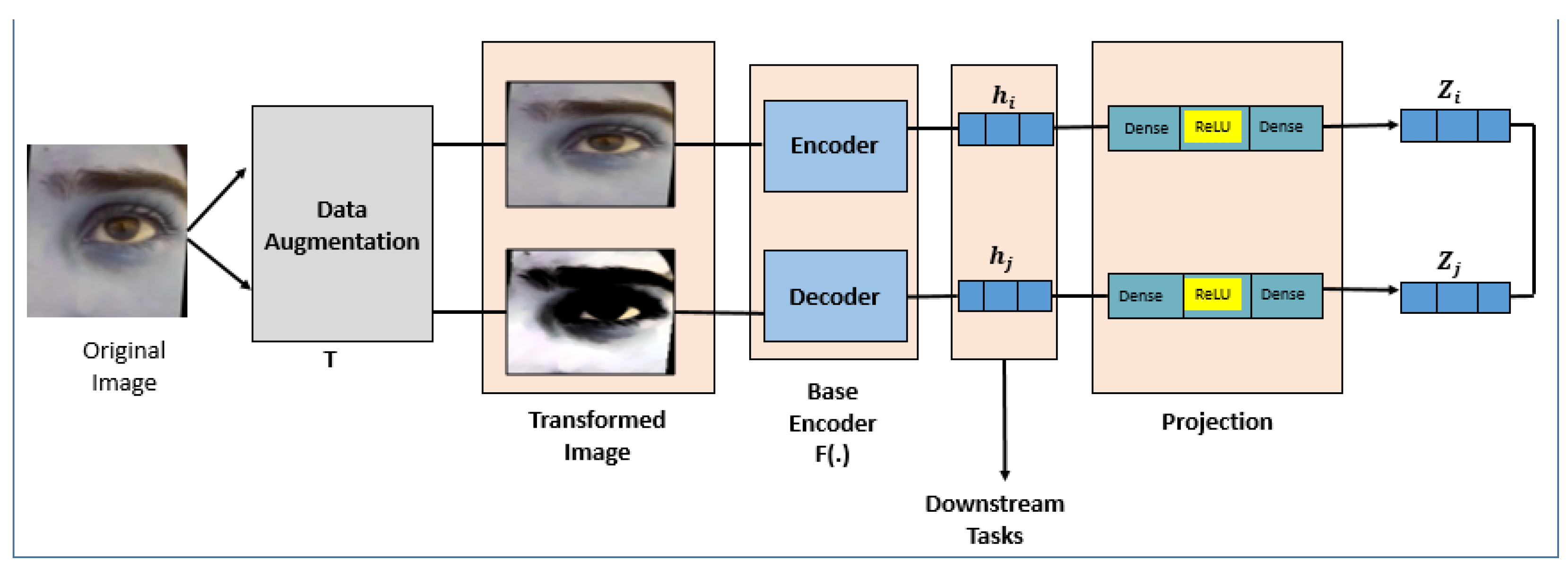
3.4.6. SimCLR: A Simple Framework for Contrastive Learning of Visual Representations

SimCLR [39], which stands for A Simple Framework for Contrastive Learning of Visual Representations, is a form of self-supervised learning. SimCLR enables models to learn from unlabeled data by generating tasks that supervise themselves, acquiring meaningful visual representations by contrasting dissimilar and similar examples, as shown in Figure 8.

The framework consists of four main steps:

• Data augmentation [40]: a single image is subjected to two distinct random augmentations, producing two augmented views of the original image, denoted as $x_i$ and $x_j$.
• Base encoder [41]: Typically a convolutional neural network, the base encoder extracts high-level feature representations from the two augmented views generated in the previous step, resulting in representations $h_i$ and $h_j$.
• Projection head: this step employs a multilayer perceptron (MLP) [42] with one hidden layer to project the feature representations $h_i$ and $h_j$ into a lower-dimensional space, facilitating the learning of more discriminative representations.
• Contrastive loss: This step optimizes the model by maximizing the similarity between positive pairs—the two augmented versions of the same image—while minimizing the similarity with negative pairs, which are augmented views of different images. Cosine similarity is used to measure the closeness between the positive pair $z_i$ and $z_j$, ensuring the model effectively differentiates between similar and dissimilar images.

3.5. Evaluation Metrics

During the training phase and for user testing, several evaluation metrics were employed to assess the performance of the models, including precision, recall, F1 score, loss, similarity, and total inference time.

The precision (P) is defined as the ratio of the correctly predicted positive observations number divided by the total predicted positives. The higher the precision, the higher the proportion of the positive predictions made by the model are correct:

$$P={\displaystyle \frac{TP}{TP+FP}}$$

(1)

where TP = true positives, FP = false positives, and FN = false negatives.

The recall(R) is defined as the ratio of correctly predicted positive observations to all the observations in the actual class. The higher the recall, the better the detection of the positive class:

$$R={\displaystyle \frac{TP}{TP+FN}}$$

(2)

The F1 score is defined as the harmonic mean of precision and recall. The F1 score is one single metric that shows precision and recall in balance for a model; we use the F1 score when we need to find the equilibrium between precision and recall:

$$F1=2\times {\displaystyle \frac{P\times R}{P+R}}$$

(3)

Similarity (S) is defined as how close the written word and the actual text word are:

$$S=1-{\displaystyle \frac{D(W_1,W_2)}{max\left(\right|W_1|,|W_2\left|\right)}}$$

(4)

where $D(W_1,W_2)$ is the Levenshtein distance and $\left|W\right|$ is the length of the word.

The total inference time is defined as how long the user takes to enter one word using one of our proposed models. The total inference time is crucial for evaluating performance, especially in real-time systems:

$$T_{total}=\sum _{i=1}^N{T}_i$$

(5)

where: $T_{t}otal$ = total inference time, $T_i$ = inference time for each input, and N = number of inputs.

The mean average precision (mAP) is defined as the average precision across multiple classes and threshold values, serving as a key metric to evaluate the performance of object detection models. The mAP is calculated as follows:

$$\mathrm{mAP}={\displaystyle \frac{1}{N}}\sum _{i=1}^{N}A{P}_i$$

(6)

where N: number of classes and $A{P}_i$: average precision for class i.

The model’s certainty that a predicted bounding box contains an object of interest is called the confidence. The confidence measures the probability that the detected object belongs to a specific class, providing a measure of prediction reliability. The higher the confidence score, the higher the detected object is correctly classified:

$$\mathrm{Confidence}=P\left(\mathrm{Object}\right)\times P(\mathrm{Class}\mid \mathrm{Object})$$

(7)

where $P\left(\mathrm{Object}\right)$: the probability that an object exists within the predicted bounding box and $P(\mathrm{Class}\mid \mathrm{Object})$: the probability that the object belongs to a specific class, given that an object exists in the bounding box.

The Intersection over Union (IoU) is defined as the ratio of the area of intersection between the predicted object and the ground truth to the area of their union. The IoU serves as a metric to assess the accuracy of a predicted bounding box in comparison to the ground truth bounding box:

$$\mathrm{IoU}={\displaystyle \frac{\mathrm{Area}\mathrm{of}\mathrm{Intersection}}{\mathrm{Area}\mathrm{of}\mathrm{Union}}}$$

(8)

The loss functions are mathematical equations employed to evaluate the disparity between the model’s predicted output and the actual ground truth. In machine learning and deep learning, the objective is to minimize various types of loss functions to achieve optimal performance from the model. One such loss function is the binary cross-entropy loss, defined as

$$\mathrm{loss}=-\left(y·log\left(\hat{y}\right)+(1-y)·log(1-\hat{y})\right)$$

(9)

where y represents the actual label and $\hat{y}$ denotes the predicted probability.

3.6. Experimental Setup

We conducted our experiments using Python for software, and as we hold many algorithms, we utilized several libraries, including Python (version 3.9.20), TensorFlow (version 2.10.0), Keras (version 2.10.0), PyTorch (version 2.0.0+cu117), torchvision (version 0.15.0+cu117), and Ultralytics (version 8.2.38). For the hardware, we used our laptop’s GPU and camera; the laptop details are listed in

Table 2. Our hardware characteristics.

Storage capacity	512 GB
Processor model	Intel Core i7
Graphics card model	NVIDIA GeForce RTX 3050 GDDR6 Graphics
Camera type	HD RGB camera

.

4. Results and Discussion

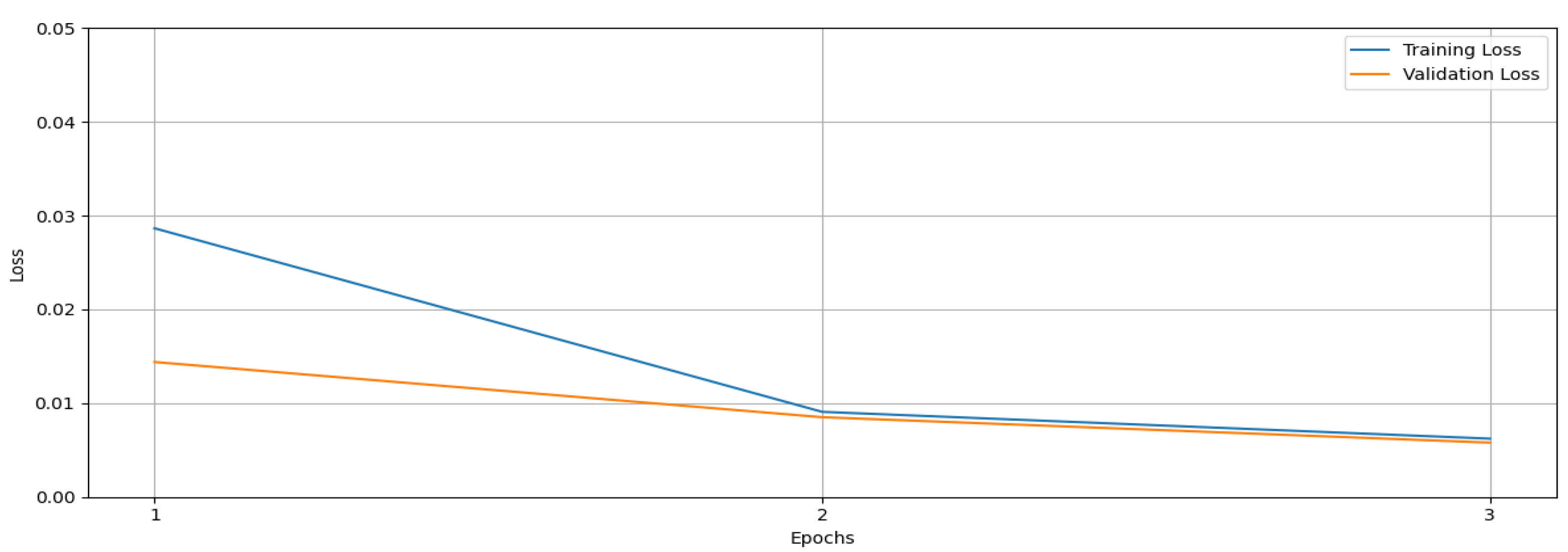
4.1. YOLOv8 Training Results

To input images into YOLOv8, it is necessary to resize all images to a resolution of 640 × 360. During the training process, we generated several performance curves to evaluate the model’s effectiveness.

The F1–confidence curve in Figure 9a measures the balance between precision and recall. All classes have an F1 score of 0.82 at a confidence of 0.179. Higher curves mean better performance. The precision–confidence curve in Figure 9b shows how many detected objects are correct. All classes have a precision of 1.00 at a confidence of 0.817. As confidence increases, precision generally improves. As shown by the precision–recall curve in Figure 9c, precision and recall balance each other. The mean average precision (mAP) for all classes is 0.829 at a recall of 0.5. The recall–confidence curve in Figure 9d shows how many actual objects were detected. All classes have a recall of 0.83 at a confidence of 0.080. Higher recall at lower confidence means the model detects more objects when less certain.

4.2. SSD Training Results

To input the images into SSD, all images were resized to 300 × 300 pixels. Figure 10 illustrates two distinct mean average precision (mAP) curves: mAP@0.5: this curve represents the mAP calculated using an Intersection over Union (IoU) threshold of 0.5, indicating the model’s capability to detect objects with a significant overlap between the predicted bounding box and the ground truth box. mAP@0.5:0.95: this curve represents the mAP calculated over an IoU threshold range from 0.5 to 0.95, evaluating the model’s performance in detecting objects at various overlap levels, including more challenging cases with lower IoU values.

4.3. Faster R-CNN Training Results

We obtained two curves to judge our model’s performance during the training process. The first chart loss of the Region Proposal Network shows the classification loss of the Region Proposal Network (RPN), as shown on the left side of Figure 11, while Figure 11 on the right side indicates the regression loss of the RPN. How well the RPN can predict the precise bounding box coordinates of the proposed regions is measured by the regression loss.

4.4. DeepLabv3 Training Results

Figure 12 explains how our model works during the training process by selecting a random image from the training to show the training process results. The sample image consists of two panels: The left image represents the raw eye input used during training. It highlights critical features such as the pupil, iris, and surrounding eye area, essential for accurate segmentation. The right image displays the segmentation mask predicted by the DeepLabv3 model. However, the uniform appearance of the mask suggests that the model might not have effectively segmented the target regions in this particular instance.

4.5. U-Net Training Results

We obtained the training and validation loss curves for the U-Net model to evaluate its performance, as depicted in Figure 13. Training loss = 0.0062: This value represents the loss computed over the training dataset, indicating how effectively the model is learning from the provided training examples. Validation loss = 0.0057: This value represents the loss calculated over the validation dataset. Since the validation dataset was not used during training, it indicates how well the model is likely to perform on unseen data. A training loss of 0.0062 and validation loss of 0.0057 suggest that the model is performing reasonably well on the training data.

4.6. SimCLR Training Results

SimCLR achieved a total loss of 94.40 during the training process. The loss function evaluates the disparity between the model’s predicted output and the actual ground truth. A higher loss generally means the model’s predictions are far from the ground truth, and a lower loss indicates better performance. That means SimCLR is not suitable for our eye-gaze detection.

4.7. User Testing and Evaluation

We check our model’s performance in real time to make sure of the speed, if we can overcome environmental obstacles like low lighting and user fatigue, and if our system is user-friendly. We asked different users with different eye shapes and sizes to try our models, and one of our users was wearing glasses. One of the biggest obstacles is that glasses reflect light, so we cannot detect exactly where the pupil is, but we used two models from the image segmentation area. To ensure consistent testing conditions across the six users and mitigate the influence of individual variability, several calibration steps were implemented:

• Initial setup calibration: The system was designed to record eye-gaze direction coordinates at four specific points—upper left, upper right, lower left, and lower right—before each trial for every user. These coordinates were subsequently utilized in the calculations to determine the user’s point of gaze precisely.
• Lighting control: Participants were instructed to complete the test under consistent lighting conditions to minimize the impact of environmental factors on eye-gaze tracking accuracy.
• Position standardization: Participants were instructed to maintain a perpendicular gaze toward the camera during testing to ensure consistent alignment and reduce variations in eye-gaze tracking.
• Eyeglass reflection handling: For the participant wearing glasses, adjustments were made to minimize reflections by altering the lighting position. The user was rotated 360 degrees to identify the optimal angle that reduced glare and ensured more accurate eye-gaze tracking.

We assigned five words to ensure our test was fair for all. Our testing vector = [WORK, TIME, GOOD, INFORMATION, DIFFERENT]. We aim to design a system that can help disabled people during their daily routine, so we picked the most used words we use every day. We intended to select short words like “WORK”, “TIME”, and “GOOD”, and long ones like “INFORMATION” and “DIFFERENT”. The user-testing experiment was designed as follows: Participants were asked to input words in a fixed order, with a one-minute timer allocated for each word. The goal was for each user to complete the entry of five words within a single session. To evaluate performance, the actual word entered by the user was compared with the written word to compute several metrics, including precision, recall, F1 score, similarity, and total inference time. We conducted a pilot study, and the conclusions refer to a preliminary model evaluation rather than final usability testing, as the focus of this study was model selection rather than generalization. This process is automated within our system, and the results are saved in an Excel file, enabling a comparison of performance across all users.

Table 3. The mean of evaluation metrics for six users.

Model	Precision	Total Inference Time (s)	Recall	F1 Score	Similarity
DeepLab	0.7252	56.1962	0.4436	0.4845	0.4214
FRCNN	0.1000	41.1021	0.0207	0.0324	0.0255
Haar	0.8881	44.4113	0.8600	0.8431	0.7474
SimCLR	0.0000	42.4106	0.0000	0.0000	0.0000
SSD	0.2988	51.1207	0.3929	0.3183	0.2334
U-Net	0.4456	48.1702	0.4125	0.4026	0.2196
YOLO	0.8235	52.6745	0.7460	0.7445	0.6733

shows that the evaluation metrics from the initial user-testing experiment were conducted with only six users to validate our findings. The reported values represent the mean performance of each model across all participants. For instance, precision 1 is calculated as

$$\mathrm{Mean}{(\mathsf{\mu })}_{\mathrm{Precision}}={\displaystyle \frac{\sum X}{N}}$$

(10)

where N represents the number of users and $\sum X$ denotes the summation of the precision values for each model across all participants.

4.7.1. Test User Analysis

Table 4. Standard deviation of performance metrics across models.

Model	SD of Precision	SD of F1	SD of Recall	SD of Total Inference Time	SD of Similarity
DeepLab	0.3304	0.2926	0.3486	10.7725	0.2467
FRCNN	0.2754	0.0855	0.0563	25.3946	0.0661
Haar	0.2041	0.1883	0.2234	12.6458	0.1830
SimCLR	0	0	0	26.6170	0
SSD	0.1568	0.1709	0.2728	12.0616	0.1298
U-Net	0.3210	0.2498	0.2496	15.7996	0.1574
YOLO	0.2155	0.2287	0.2874	9.7165	0.2524

offers the standard deviation (SD), which provides some insights into our small user test dataset and highlights a few key points:

$$SD=\sqrt{{\displaystyle \frac{\sum {(X-\mathsf{\mu })}^2}{N}}}$$

(11)

where N: represents the number of users, X: denotes each value of the measuring matrix for each model across all participants, and $\mathsf{\mu }$ denotes the mean of each measuring matrix for each model across all participants.

The notable variability among users indicates that increasing the sample size could enhance the reliability of performance estimates for each model. However, YOLO and Haar consistently demonstrated stability, exhibiting relatively low standard deviation (SD) values in comparison to their already high precision and F1 scores. The reported SD values support our assertion that expanding the number of users did not significantly impact the performance of the top-performing models. Conversely, the higher variability observed in weaker models underscores their instability, suggesting the potential benefit of additional data. Nevertheless, as our focus will be on the superior models in subsequent stages, further expansion of the user-testing process is deemed unnecessary.

4.7.2. Similarity Score Analysis

• YOLO: as shown in Figure 14, Achieves a median similarity score around $0.7$–$0.8$, with some scores reaching $1.0$. This indicates that YOLO effectively balances speed and accuracy, making it suitable for real-time applications requiring high detection precision.
• Haar: Shows a stable performance with a median similarity score around $0.7$ and a range between $0.4$ and $1.0$. Its robust performance could be attributed to its feature-based approach, which works well with structured patterns, particularly in face and object detection tasks.
• DeepLab: The median similarity score is about $0.4$, but the high variability (ranging from 0 to $0.8$) indicates an inconsistent performance. This variability could stem from its reliance on pixel-wise classification, which can struggle with fine object boundaries and diverse backgrounds.
• SSD: Achieves a median similarity around $0.3$, reflecting a moderate performance. SSD trades off accuracy for faster inference by detecting objects in a single shot, which may explain its lower similarity scores compared to YOLO and Haar.
• U-Net: shows a lower median similarity score of about $0.2$–$0.3$, likely due to its design for segmentation tasks rather than object detection, making it less effective in capturing object boundaries in this context.
• SimCLR and FRCNN: Both models have similarity scores close to 0, indicating poor performance in this task. SimCLR, as a contrastive learning model, focuses on learning feature representations rather than direct object detection. Similarly, Faster R-CNN’s performance might be hindered by its complex two-stage architecture, leading to slower inference and missed detections in real-time scenarios.

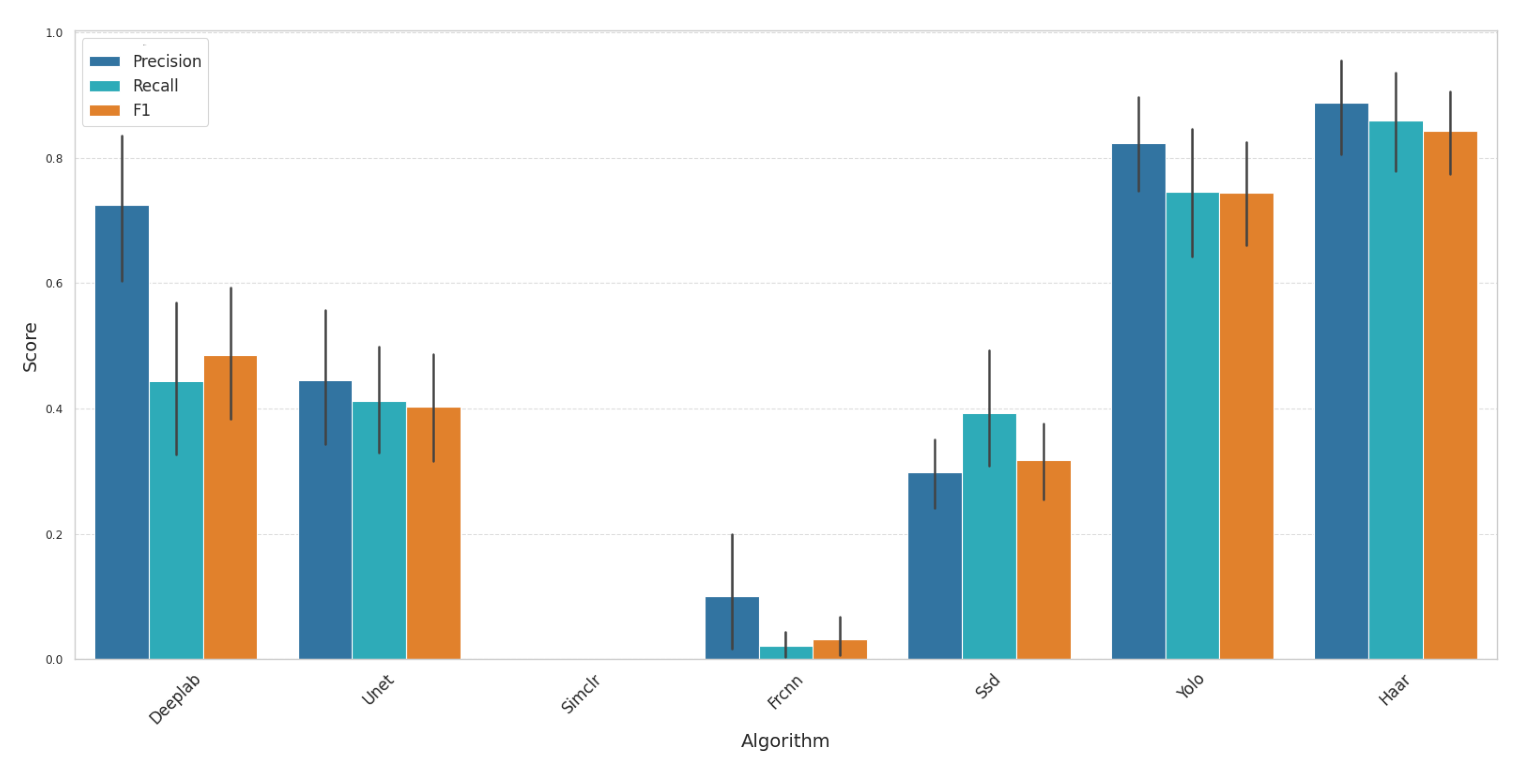
4.7.3. Precision, Recall, and F1 Score Analysis

The performance of the models was evaluated using precision, recall, and F1 scores to assess their effectiveness in object detection tasks, Figure 15. The analysis is summarized as follows:

• Haar demonstrated the best overall performance, achieving the highest scores across all metrics: precision: 0.88, recall: 0.86, and F1 score: 0.85. This can be attributed to Haar’s effective feature-based detection, which excels in structured environments with distinct object boundaries.
• YOLO also performed very well, presenting itself as a strong alternative. It achieved a precision of 0.85, a recall of 0.80, and an F1 score of 0.80. YOLO’s real-time detection capability, combined with its balance of speed and accuracy, makes it suitable for applications requiring rapid responses with reliable accuracy.
• DeepLab and U-Net showed a moderate performance but lacked consistency. DeepLab achieved a precision of 0.70, recall of 0.48, and F1 score of 0.55. These models are primarily designed for segmentation tasks, which may explain their reduced effectiveness in object detection tasks, especially in detecting fine-grained features.
• SSD, Faster R-CNN, and SimCLR performed poorly. SSD’s single-shot architecture sacrifices accuracy for speed, resulting in lower precision and recall. Faster R-CNN, despite its two-stage detection process, struggled with speed and accuracy balance, leading to suboptimal results. SimCLR showed no effectiveness in this context, as its focus on contrastive learning is less suited for direct object detection.

Figure 15. Precision, recall, and F1 score for each algorithm.

Figure 15. Precision, recall, and F1 score for each algorithm.

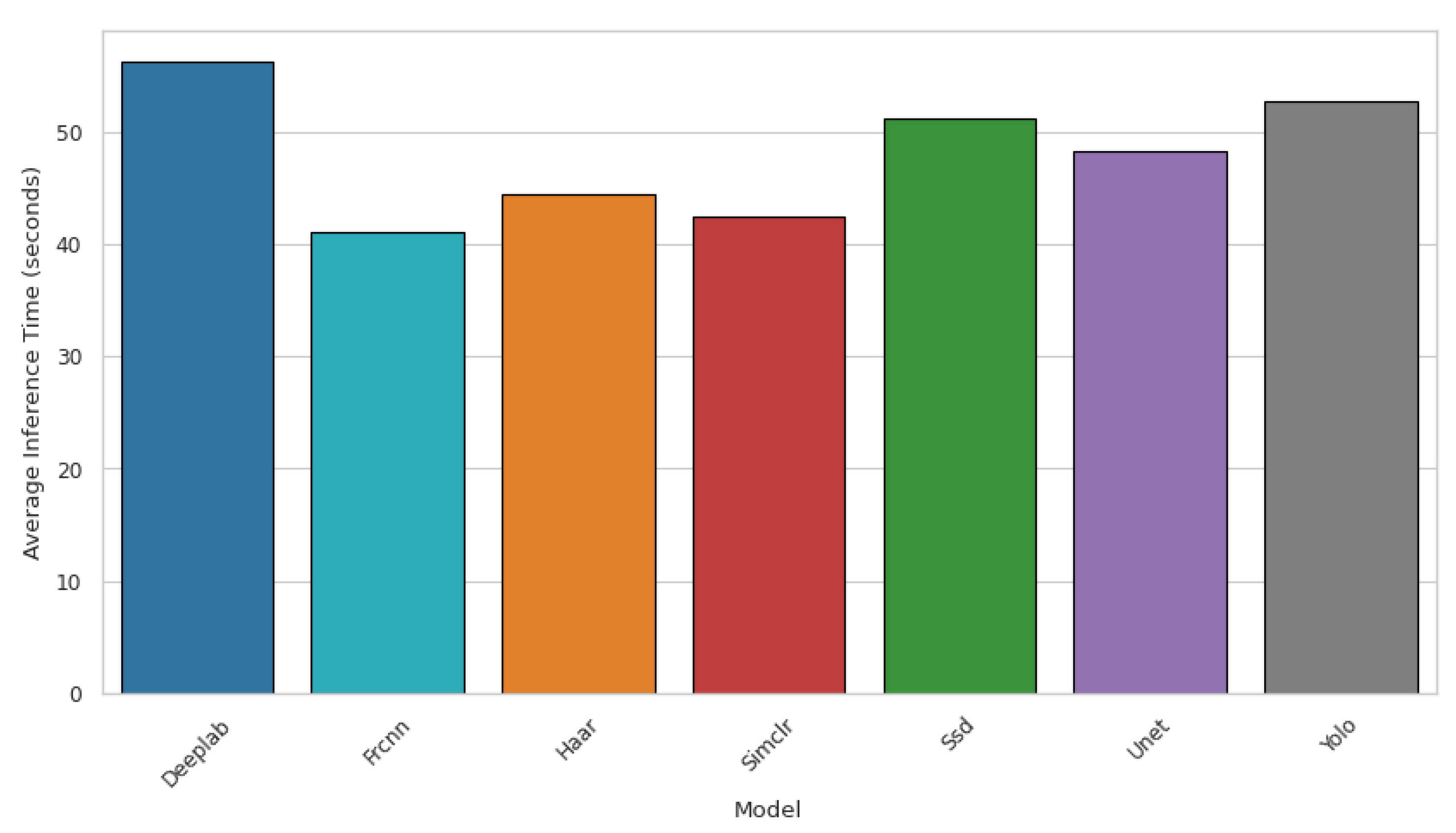
4.7.4. Total Inference Time

Figure 16 illustrates the average time required for each model to process the word input vector across all users. The inference time of a model is a crucial factor in real-time applications, but a shorter inference time does not necessarily indicate a better overall performance. While models like Faster R-CNN and SimCLR have relatively lower inference times, their similarity scores and F1 scores are significantly lower, making them unsuitable for tasks requiring high accuracy. YOLOv8 and Haar have slightly higher inference times; however, they demonstrate superior similarity scores and F1 scores, making them more reliable choices. DeepLab and U-Net have a reasonable performance and longer inference times, which might impact real-time applications. Thus, model selection should balance accuracy, similarity, inference time, and model size rather than focusing solely on speed.

4.8. Comparison of ALL Model Results

The model size is a critical consideration in our case, as our objective is to develop an affordable real-time eye-gaze writing system that can be deployed on smartphones. A compact model size in memory would be beneficial, particularly if we enhance our system with features such as text suggestions or text-to-speech capabilities.

Table 5. Comparison of the proposed models.

Model	Precision	Recall	F1 Score	Inference Time (s)	Model Size (KB)	Performance Evaluation	Usability
Haar	0.85	0.83	0.85	45	97.358	Best overall (high accuracy and reasonable speed)	Best choice
YOLOv8	0.88	0.80	0.83	52	6.083	High accuracy and smallest model	Best compact model
DeepLabv3	0.72	0.50	0.82	55	238.906	High accuracy but large model and slow	Inefficient
U-Net	0.50	0.42	0.84	48	121.234	Moderate accuracy, large size	Not ideal
Faster R-CNN	0.15	0.05	0.82	41	534.013	Too large model, low efficiency	Avoid
SSD	0.40	0.38	0.49	51	87.071	Low accuracy, moderate size	Poor choice
SimCLR	0.05	0.02	0.77	43	45.327	Worst accuracy, poor similarity	Avoid

presents a comparative analysis of the proposed models, evaluating their performance based on model size, F1 score, recall, total inference time, and overall efficiency.

The Haar Cascade Classifier demonstrates simplicity and effectiveness in object detection by leveraging handcrafted features specifically designed to identify high-contrast regions, such as eyes or faces. This makes Haar particularly well-suited for controlled environments. Moreover, its reliance on predefined feature extraction reduces false positives compared to deep learning models, which often require extensive datasets to achieve optimal generalization.

Although Haar achieves a marginally higher F1 score, YOLOv8 offers a more balanced trade-off between accuracy, inference speed, and model size. Its faster processing time and significantly smaller model size make it preferable for real-time applications where computational efficiency is crucial.

In contrast, models such as SSD and Faster R-CNN exhibit higher susceptibility to misinterpreting background elements, leading to an increased rate of false detections. SimCLR, on the other hand, performs poorly in this context due to its reliance on contrastive learning, which is not well optimized for fine-grained object detection tasks, such as identifying eye pupils.

The selection of the optimal model ultimately depends on the application’s requirements regarding the balance between speed and accuracy. Haar is ideal in scenarios where accuracy is paramount and environmental conditions are controlled, while YOLOv8 emerges as the more practical choice for real-time applications that demand a lightweight architecture and faster inference.

5. Conclusions

Our analysis revealed that Haar and YOLOv8 demonstrated the best overall performance, achieving high F1 scores with reasonable inference times. Haar’s handcrafted features make it particularly effective in controlled environments, especially for detecting high-contrast features like eyes or faces, resulting in fewer false positives. YOLOv8, on the other hand, balances accuracy, inference speed, and compact model size, making it highly suitable for real-time applications, particularly on resource-constrained devices. In contrast, DeepLabv3 and U-Net exhibited moderate accuracy but suffered from larger model sizes and slower inference times, limiting their practicality for real-time use. SSD and Faster R-CNN demonstrated lower accuracy, making them less suitable for tasks requiring high precision. SimCLR performed the worst, indicating its inefficiency in similarity detection tasks due to its reliance on contrastive learning, which is less effective for fine-grained object detection like pupil tracking. It is important to note that a shorter inference time does not necessarily imply a better model, as seen with Faster R-CNN, which exhibited low latency but poor accuracy. This study also highlights the significance of model size for deployment on devices with limited computational resources, with YOLOv8 emerging as a compelling choice due to its compact size and high accuracy. Based on the results, Haar and YOLOv8 emerge as the most suitable choices, offering a balance between accuracy, efficiency, and model size. Haar is ideal for scenarios prioritizing accuracy in controlled environments, while YOLOv8 excels in real-time applications. SSD could be considered for use cases where speed is prioritized over accuracy, but Faster R-CNN and SimCLR should be avoided due to their poor performance.

We propose several avenues for future work, such as YOLOv12 and developing an integrated system that combines gaze prediction with text suggestions to improve usability. Future work should focus on text suggestions with the selected models at typical writing speeds. At the final stage, we aim to design a floating keyboard so disabled people can use smartphones and connect our system with text-to-voice systems.

References

1. Nerişanu, R.A.; Cioca, L.I. A Better Life in Digital World: Using Eye-Gaze Technology to Enhance Life Quality of Physically Disabled People. In Digital Transformation: Exploring the Impact of Digital Transformation on Organizational Processes; Springer: Berlin/Heidelberg, Germany, 2024; pp. 67–99. [Google Scholar]
2. Paraskevoudi, N.; Pezaris, J.S. Eye movement compensation and spatial updating in visual prosthetics: Mechanisms, limitations, and future directions. Front. Syst. Neurosci. 2019, 12, 73. [Google Scholar] [CrossRef] [PubMed]
3. Zhang, C.; Chi, J.N.; Zhang, Z.H.; Wang, Z.L. A novel eye gaze tracking technique based on pupil center cornea reflection technique. Jisuanji Xuebao—Chin. J. Comput. 2010, 33, 1272–1285. [Google Scholar] [CrossRef]
4. Zhu, Z.; Ji, Q. Eye gaze tracking under natural head movements. In Proceedings of the 2005 IEEE Computer Society Conference on Computer Vision and Pattern Recognition (CVPR’05), San Diego, CA, USA, 20–25 June 2005; Volume 1, pp. 918–923. [Google Scholar]
5. Roth, P.M.; Winter, M. Survey of Appearance-Based Methods for Object Recognition; Technical Report ICGTR0108 (ICG-TR-01/08); Institute for Computer Graphics and Vision, Graz University of Technology: Graz, Austria, 2008. [Google Scholar]
6. Fischer, T.; Chang, H.J.; Demiris, Y. Rt-gene: Real-time eye gaze estimation in natural environments. In Proceedings of the European Conference on Computer Vision (ECCV), Munich, Germany, 8–14 September 2018; pp. 334–352. [Google Scholar]
7. Wang, Y.; Shen, T.; Yuan, G.; Bian, J.; Fu, X. Appearance-based gaze estimation using deep features and random forest regression. Knowl.-Based Syst. 2016, 110, 293–301. [Google Scholar] [CrossRef]
8. Salvucci, D.D.; Goldberg, J.H. Identifying fixations and saccades in eye-tracking protocols. In Proceedings of the 2000 Symposium on Eye Tracking Research & Applications, Palm Beach Gardens, FL, USA, 6–8 November 2000; pp. 71–78. [Google Scholar]
9. Hansen, D.W.; Ji, Q. In the eye of the beholder: A survey of models for eyes and gaze. IEEE Trans. Pattern Anal. Mach. Intell. 2009, 32, 478–500. [Google Scholar] [CrossRef] [PubMed]
10. Zhang, X.; Sugano, Y.; Bulling, A. Evaluation of appearance-based methods and implications for gaze-based applications. In Proceedings of the 2019 CHI Conference on Human Factors in Computing Systems, Glasgow, UK, 4–9 May 2019; pp. 1–13. [Google Scholar]
11. Whitehill, J.; Omlin, C.W. Haar features for FACS AU recognition. In Proceedings of the 7th International Conference on Automatic Face and Gesture Recognition (FGR06), Southampton, UK, 24 April 2006; p. 5. [Google Scholar]
12. Li, Y.; Xu, X.; Mu, N.; Chen, L. Eye-gaze tracking system by haar cascade classifier. In Proceedings of the 2016 IEEE 11th Conference on Industrial Electronics and Applications (ICIEA), Hefei, China, 5–7 June 2016; pp. 564–567. [Google Scholar]
13. Ngo, H.T.; Rakvic, R.N.; Broussard, R.P.; Ives, R.W. An FPGA-based design of a modular approach for integral images in a real-time face detection system. In Proceedings of the Mobile Multimedia/Image Processing, Security, and Applications 2009, Orlando, FL, USA, 13–17 April 2009; Volume 7351, pp. 83–92. [Google Scholar]
14. Bulling, A. DaRUS Dataset: Eye-Gaze Writing Models. Available online: https://darus.uni-stuttgart.de/dataset.xhtml?persistentId=doi:10.18419/darus-3230&version=1.0 (accessed on 1 March 2025).
15. RoboFlow. Eyes Dataset. Available online: https://universe.roboflow.com/rethinkai2/eyes-mv4fm/dataset/1 (accessed on 1 March 2025).
16. RoboFlow. Dataset Pupil. Available online: https://universe.roboflow.com/politeknik-negeri-padang-yeiym/dataset-pupil (accessed on 1 March 2025).
17. RoboFlow. Pupil Detection Dataset. Available online: https://universe.roboflow.com/rocket-vhngd/pupil-detection-fqerx (accessed on 1 March 2025).
18. RoboFlow. Pupils Dataset. Available online: https://universe.roboflow.com/artem-bdqda/pupils-3wyx2/dataset/5 (accessed on 1 March 2025).
19. Wang, G.; Chen, Y.; An, P.; Hong, H.; Hu, J.; Huang, T. UAV-YOLOv8: A small-object-detection model based on improved YOLOv8 for UAV aerial photography scenarios. Sensors 2023, 23, 7190. [Google Scholar] [CrossRef] [PubMed]
20. Redmon, J. Yolov3: An incremental improvement. arXiv 2018, arXiv:1804.02767. [Google Scholar]
21. He, K.; Zhang, X.; Ren, S.; Sun, J. Spatial pyramid pooling in deep convolutional networks for visual recognition. IEEE Trans. Pattern Anal. Mach. Intell. 2015, 37, 1904–1916. [Google Scholar] [CrossRef] [PubMed]
22. Liu, S.; Qi, L.; Qin, H.; Shi, J.; Jia, J. Path aggregation network for instance segmentation. In Proceedings of the IEEE Conference on Computer Vision and Pattern Recognition, Salt Lake City, UT, USA, 18–23 June 2018; pp. 8759–8768. [Google Scholar]
23. Li, X.; Wang, W.; Wu, L.; Chen, S.; Hu, X.; Li, J.; Tang, J.; Yang, J. Generalized focal loss: Learning qualified and distributed bounding boxes for dense object detection. Adv. Neural Inf. Process. Syst. 2020, 33, 21002–21012. [Google Scholar]
24. Zheng, Z.; Wang, P.; Liu, W.; Li, J.; Ye, R.; Ren, D. Distance-IoU loss: Faster and better learning for bounding box regression. In Proceedings of the AAAI Conference on Artificial Intelligence, New York, NY, USA, 7–12 February 2020; Volume 34, pp. 12993–13000. [Google Scholar]
25. Feng, C.; Zhong, Y.; Gao, Y.; Scott, M.R.; Huang, W. Tood: Task-aligned one-stage object detection. In Proceedings of the 2021 IEEE/CVF International Conference on Computer Vision (ICCV), Montreal, BC, Canada, 11–17 October 2021; pp. 3490–3499. [Google Scholar]
26. Liu, W.; Anguelov, D.; Erhan, D.; Szegedy, C.; Reed, S.; Fu, C.Y.; Berg, A.C. Ssd: Single shot multibox detector. In Proceedings of the Computer Vision–ECCV 2016: 14th European Conference, Amsterdam, The Netherlands, 11–14 October 2016; Proceedings, Part I 14. Springer: Berlin/Heidelberg, Germany, 2016; pp. 21–37. [Google Scholar]
27. Zhai, S.; Shang, D.; Wang, S.; Dong, S. DF-SSD: An improved SSD object detection algorithm based on DenseNet and feature fusion. IEEE Access 2020, 8, 24344–24357. [Google Scholar] [CrossRef]
28. Theckedath, D.; Sedamkar, R. Detecting affect states using VGG16, ResNet50 and SE-ResNet50 networks. SN Comput. Sci. 2020, 1, 79. [Google Scholar] [CrossRef]
29. Jia, Y.; Shelhamer, E.; Donahue, J.; Karayev, S.; Long, J.; Girshick, R.; Guadarrama, S.; Darrell, T. Caffe: Convolutional architecture for fast feature embedding. In Proceedings of the 22nd ACM International Conference on Multimedia, Orlando, FL, USA, 3–7 November 2014; pp. 675–678. [Google Scholar]
30. Lee, C.; Kim, H.J.; Oh, K.W. Comparison of faster R-CNN models for object detection. In Proceedings of the 2016 16th International Conference on Control, Automation and Systems (ICCAS), Gyeongju, Republic of Korea, 16–19 October 2016; pp. 107–110. [Google Scholar]
31. Girshick, R. Fast r-cnn. arXiv 2015, arXiv:1504.08083. [Google Scholar]
32. Mijwil, M.M.; Aggarwal, K.; Doshi, R.; Hiran, K.K.; Gök, M. The Distinction between R-CNN and Fast RCNN in Image Analysis: A Performance Comparison. Asian J. Appl. Sci. 2022, 10, 429–437. [Google Scholar]
33. Garcia-Garcia, A.; Orts-Escolano, S.; Oprea, S.; Villena-Martinez, V.; Garcia-Rodriguez, J. A review on deep learning techniques applied to semantic segmentation. arXiv 2017, arXiv:1704.06857. [Google Scholar]
34. Du, G.; Cao, X.; Liang, J.; Chen, X.; Zhan, Y. Medical Image Segmentation based on U-Net: A Review. J. Imaging Sci. Technol. 2020, 64, jist0710. [Google Scholar] [CrossRef]
35. Ronneberger, O.; Fischer, P.; Brox, T. U-net: Convolutional networks for biomedical image segmentation. In Proceedings of the Medical Image Computing and Computer-Assisted Intervention–MICCAI 2015: 18th International Conference, Munich, Germany, 5–9 October 2015; Proceedings, Part III 18. Springer: Berlin/Heidelberg, Germany, 2015; pp. 234–241. [Google Scholar]
36. He, J.; Li, L.; Xu, J.; Zheng, C. ReLU deep neural networks and linear finite elements. arXiv 2018, arXiv:1807.03973. [Google Scholar]
37. Christlein, V.; Spranger, L.; Seuret, M.; Nicolaou, A.; Král, P.; Maier, A. Deep generalized max pooling. In Proceedings of the 2019 International Conference on Document Analysis and Recognition (ICDAR), Sydney, Australia, 20–25 September 2019; pp. 1090–1096. [Google Scholar]
38. Zhou, D.X. Theory of deep convolutional neural networks: Downsampling. Neural Netw. 2020, 124, 319–327. [Google Scholar] [CrossRef] [PubMed]
39. Chen, T.; Kornblith, S.; Norouzi, M.; Hinton, G. A simple framework for contrastive learning of visual representations. In Proceedings of the International Conference on Machine Learning, Virtual, 13–18 July 2020; pp. 1597–1607. [Google Scholar]
40. Jiang, W.; Zhang, K.; Wang, N.; Yu, M. MeshCut data augmentation for deep learning in computer vision. PLoS ONE 2020, 15, e0243613. [Google Scholar] [CrossRef] [PubMed]
41. Yeh, C.H.; Hong, C.Y.; Hsu, Y.C.; Liu, T.L.; Chen, Y.; LeCun, Y. Decoupled contrastive learning. In Proceedings of the European Conference on Computer Vision, Tel Aviv, Israel, 23–27 October 2022; pp. 668–684. [Google Scholar]
42. Taud, H.; Mas, J.F. Multilayer perceptron (MLP). In Geomatic Approaches for Modeling Land Change Scenarios; Springer: Berlin/Heidelberg, Germany, 2017; pp. 451–455. [Google Scholar]
Figure 1. Haar features used for Viola Jones’s face detection method.
Sci 07 00047 g001
Figure 3. The network structure of YOLOv8.
Sci 07 00047 g003
Figure 4. Architecture of SSD model.
Sci 07 00047 g004
Figure 5. Architecture of Faster R-CNN model.
Sci 07 00047 g005
Figure 6. Architecture of DeepLabV3 with a ResNet101 backbone.
Sci 07 00047 g006
Figure 7. The U-Net architecture, in which each multi-channel feature map is represented by a gray box.
Sci 07 00047 g007
Figure 8. SimCLR architecture.
Sci 07 00047 g008
Figure 9. YOLOv8 performance curves. (a) F1–confidence curve, (b) precision–confidence curve, (c) precision–recall curve, (d) recall–confidence curve.
Sci 07 00047 g009
Figure 10. The mean average precision for SSD.
Sci 07 00047 g010
Figure 11. Left part RPN losses and right part RPN losses for Faster R-CNN.
Sci 07 00047 g011
Figure 12. DeepLabv3 sample during training.
Sci 07 00047 g012
Figure 13. U-Net losses curve.
Sci 07 00047 g013
Figure 14. Distribution of similarity scores by algorithm.
Sci 07 00047 g014
Figure 16. Distribution of similarity scores by algorithm.
Sci 07 00047 g016