3.2. Data
The current study was conducted using a dataset concluded from a survey of 18 neighborhoods of different urban form types including traditional, in-between, and new developments in Tehran, Istanbul, and Cairo carried out in the first half of 2017. The above three eras were initiated slightly differently due to political, socio-economic, and urban planning-related phenomena in the three countries. The neighborhood selection was done in a way that 2 neighborhoods of each era were taken in each city using the following eras: Tehran: before 1930, 1930–1980, and after 1980; Istanbul: before 1950, 1950–1980, and after 1980; Cairo: before 1869, 1869–1975, and after 1975 (traditional, in-between, and new development, respectively). The dates refer to the periods when the neighborhoods were developed or virtually took their final form. According to this typology, “traditional urban form” is defined as a sort of neighborhood that is seen in the historical cores of cities or old rural areas subjected to urban growth. Many of these neighborhoods have a discernible neighborhood center (particularly in Cairo and Tehran) and are fairly compact. The buildings of such neighborhoods are attached to one another and no leapfrog developments are seen within the texture of this typical neighborhood. The second type of urban form, “in-between”, consists of semi-grid street networks with lower population and/or construction compactness compared to traditional neighborhoods. Finally, the third urban form type, “new development”, includes centerless neighborhoods, the majority of which have full-grid street networks.
The data collection was undertaken using direct questioning (face-to-face interviews). Responders were interviewed on the streets of the selected case-study neighborhoods. We attempted to interview the residents of case neighborhoods randomly, but at the same time, interviewers tried to talk to people of diverse ages and genders. Prior to the main survey, a pilot survey of 200 interviews was conducted in five neighborhoods of the three cities to make the questions and options more precise. After the main survey, 8284 validated subjects (Tehran: 2717, Istanbul: 2781, and Cairo: 2786) were acquired after validation and data cleaning. The average age of the respondents was 35.2 years in Cairo, 35.9 in Istanbul, and 38.1 in Tehran. The car ownership rate in the Istanbul sample was lower than in the Tehran and Cairo samples (0.7, 1, and 1.2, respectively). The number of driving licenses per household in Tehran (≈2.5) was considerably higher than in the other two cities. Basically, 24 continuous and 23 categorical variables were generated at the first step according to the raw data of the questionnaire and the land use quantifications. The 24 developed continuous variables were age, household car ownership, no. of driving licenses in household, household income, monthly living cost, frequency of commute trips, no. of non-work activities, last relocation time, commuting distance (m), intersection density (nodes/ha), link-node ratio, street length density (m/ha), no. of accessed facilities, no. of accessed bakeries, no. of accessed clinics, no. of accessed mosques, no. of accessed parks, no. of accessed schools, access to bakeries (m), access to mosques (m), access to clinics (m), access to schools (m), access to parks (m), and access to facilities (m). The 23 categorical variables were gender, activity, individual driving license ownership, commute mode choice, reason for car use, shopping-entertainment place inside the neighborhood, attractive shopping centers in neighborhood, frequency of public transit trips, subjective security of public transport, residential location choice, shopping-entertainment mode choice outside neighborhood, reason for not cycling, entertainment place, reason for no social activity in neighborhood, reason for public transit use, reason for no public transit use, reason for not walking, shopping-entertainment mode choice outside neighborhood, shopping-entertainment mode choice in neighborhood, shopping-entertainment mode choice in neighborhood, sense of belonging to neighborhood, cycling, and neighborhood attractiveness perception.
The final overall sample included between 420 and 476 subjects for each neighborhood. The number of subjects in each neighborhood sub-sample consisted of between 5.1% and 5.7% of the overall sample. The number of interviews in each neighborhood sub-sample made up 0.39% (Basaksehir and Basak in Istanbul) to 2.59% (Golestan-Sharghi in Tehran) of the actual inhabitants of the neighborhood. However, for the household variables, the actual proportion of respondents of each neighborhood is around four times higher dependent on the household size of the related city. The neighborhood-level confidence intervals of the findings were 4.5% to 4.7% for individual variables and 1.8% to 2.4% for household variables. In summary, all of the sample sizes of the neighborhoods are representative considering the inhabitants of all age groups living in them, with a confidence level of less than 5%. The overall sample is representative of the population of all ages of the three cities, with a confidence level of 1.08%, though this representativeness at this level remains theoretical and only the neighborhood-level representativeness should be relied on in this study. The full details of the survey were already published [
35].
In order to measure the commute distances of the respondents, information about the nearest intersection or landmark to their living and working places were collected at the end of the interviews. This was carried out in order to ensure the participants’ privacy. The two last questions of the survey instrument that were meant to collect this information were “please sign the place of the nearest intersection of streets to your house on Map 1 (attached)” and “if you work or study, please sign the place of the nearest intersection of streets to your working place on Map 2 (attached)”. Since the second question was conditional, 62.2% of the respondents answered this question. The interviewers signed the places on the neighborhood and city maps. Then, the survey office staff estimated the commuting distances based on street networks by means of ArcGIS software. In this method of calculating commute length, the most important factor is the objective value of distance, while other issues like speed, preferences, or modes are assumed to be ineffective. The reason is that such issues are included in the model in other variables; hence, including them in commute distance would cause multicollinearity. The output lengths produced a disaggregate variable for commuters.
Table 1 shows the descriptive statistics of the commute travel lengths of the overall sample and
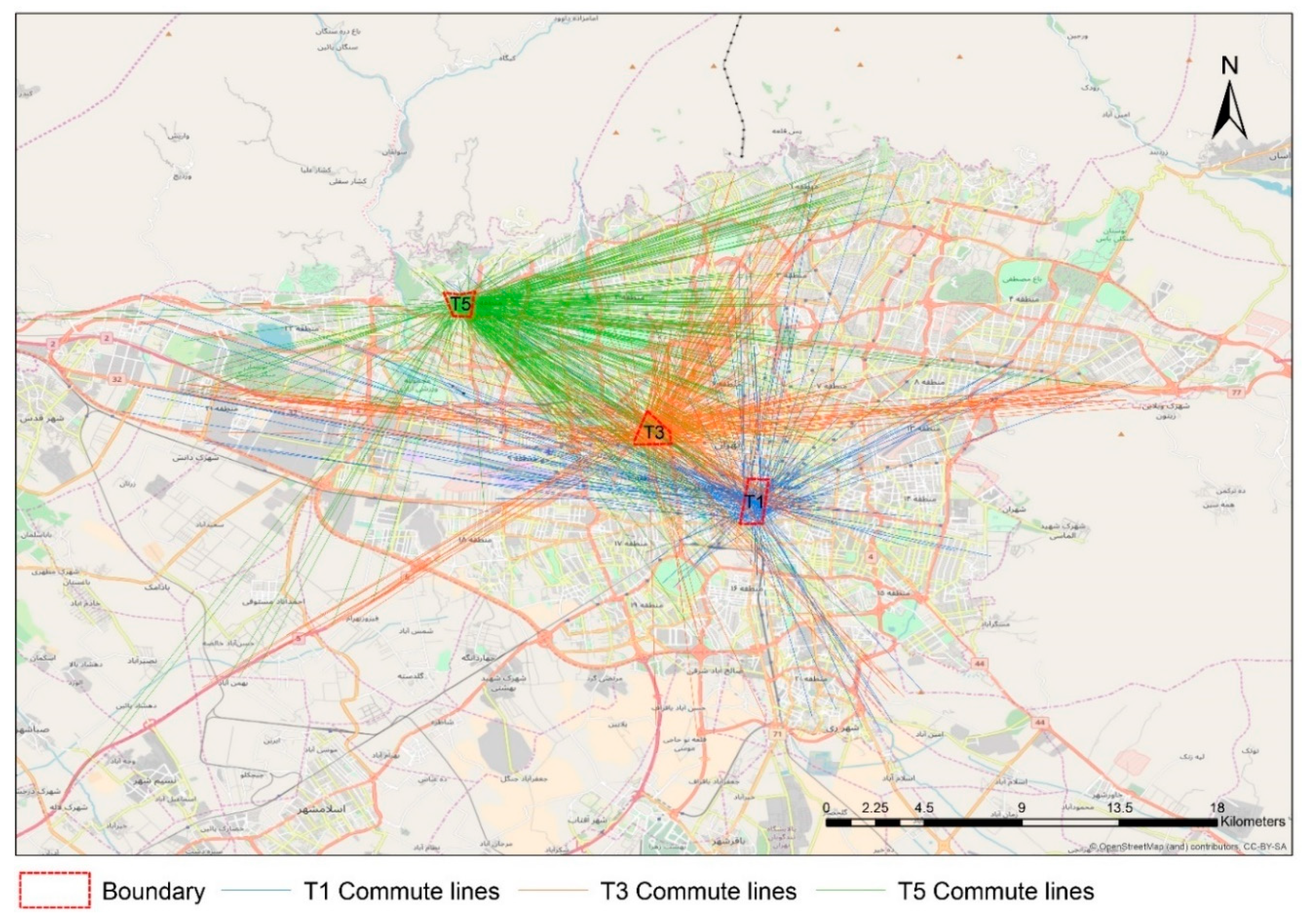
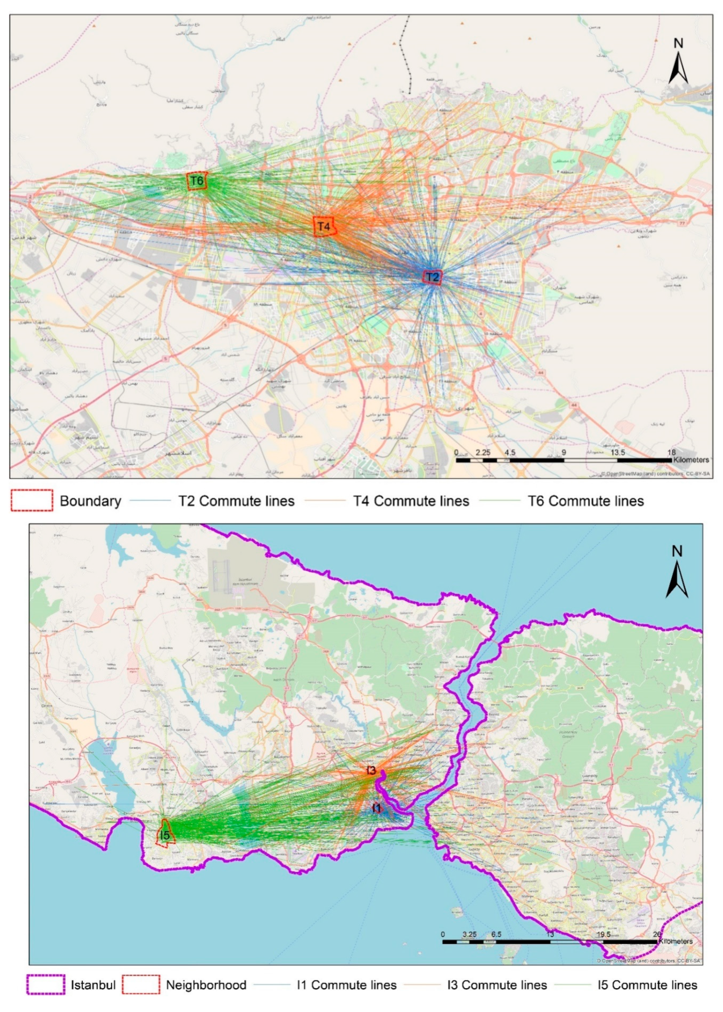
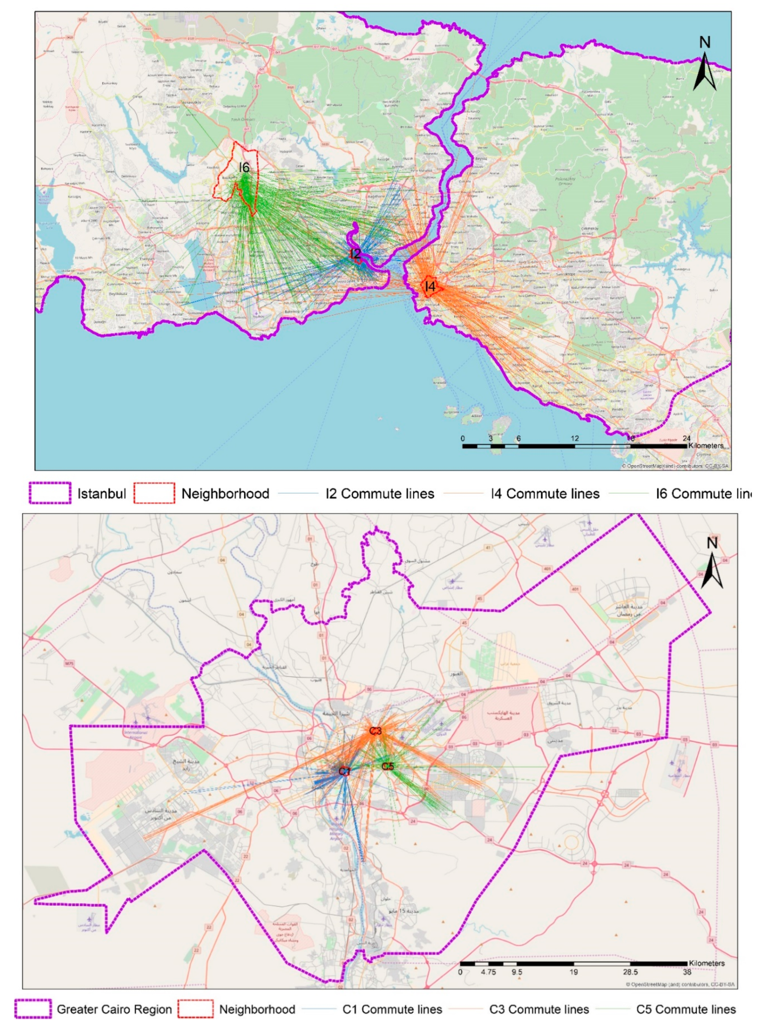
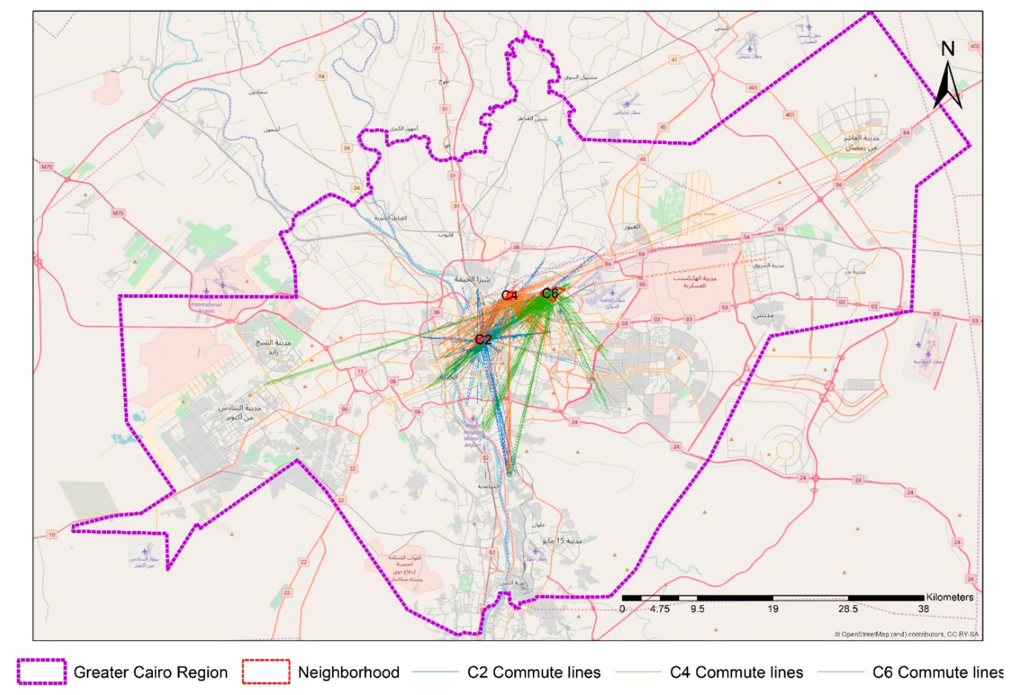
Figure 1 shows the aerial lines from the nearest street intersection to houses to the nearest intersection to workplaces by aerial lines. In this illustration, aerial lines were applied only to increase the readability of the maps. In the models, distances based on street networks were measured. The results of the Kolmogorov–Smirnov test of normality reject the hypothesis of the existence of normal distribution (statistic: 0.156, df: 5123, and
p < 0.001). Knowing whether or not the data are normal is important when selecting the analysis methods. For non-normal data, parametric methods of hypothesis testing are usually not applied. Thus, for comparing the commute distances in the three cities (research question 2), T-tests were not appropriate. Instead, the Kruskal–Wallis test was applied.
3.3. Modeling and Analysis Methods
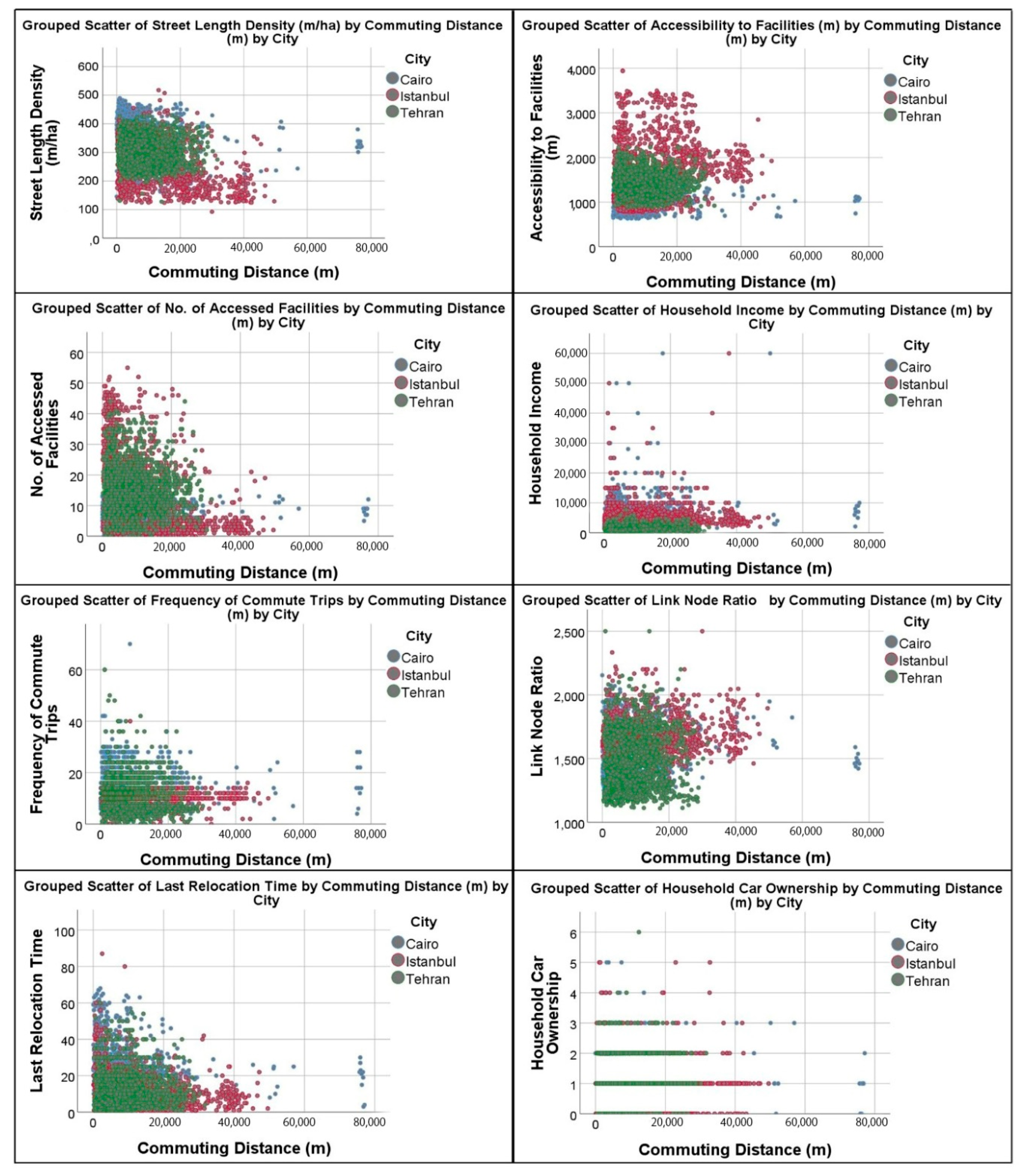
In order to answer the first research question of this study, the weighted least squares (WLS) method was applied to model commuting distances. WLS was applied because of the existence of heteroscedasticity in the commute distance variable. This problem was detected by checking the overall distribution of the variable and using four heteroscedisticity tests. The general controlling of the distribution shows a clear heteroscedasticity problem in the distribution (
Figure 2). However, to confirm the existence of the problem, heteroscedisticity tests were applied to the commute distance variable in a univariate linear regression, with all the continuous variables as covariates. We used the White test (chi-square = 305.2, df = 166,
p < 0.001), modified Breusch–Pagan test (chi-square = 65.5, df = 1,
p < 0.001), Breusch–Pagan test (chi-square = 431.4, df = 1,
p < 0.001), and F Test for heteroscedasticity (Chi-square = 66.5, df = 1,
p < 0.001). The results of all four tests highly significantly reject the null hypothesis of the homoscedasticity of the distribution. Thus, WLS was applied instead of ordinary least squares (OLS).
The dependent variable was the commute distance measured by meter. Twenty-four variables were chosen as explanatory variables at the first step and a preliminary model was generated using SPSS version 25. The modeling was conducted in 6 iterations, in each of which one or two variables with the highest
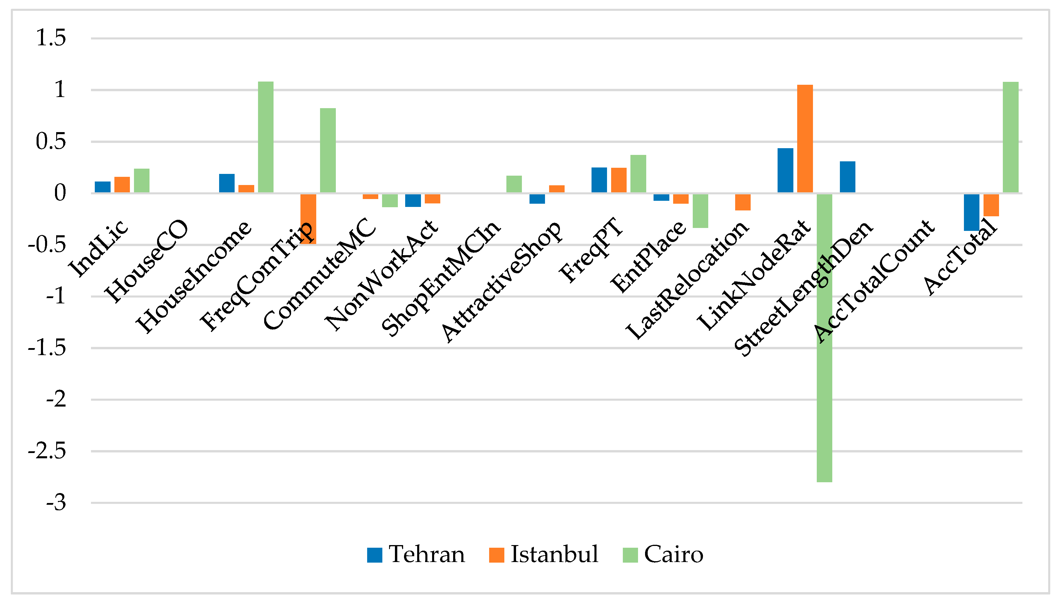
p-values were eliminated from the model to reach the highest R². The 6th model that included 14 explanatory variables generated the best results, including pseudo R² and significance of variables. The most important eliminated variables were gender, household monthly living costs, shopping-entertainment mode choice in neighborhood, shopping-entertainment mode choice outside neighborhood, and intersection density. The significance levels were 0.05 and the weights were allocated to the dependent variable (commute distances) ranging from −2 to 2 by in-between steps of 0.5 each. The WLS models included continuous and dummy variables. The continuous variables were kept as they were after data calibration and validation. The dummy variables were generated by coding categorical variables.
Table 2 illustrates the descriptive statistics of the continuous explanatory variables.
Table 3 summarizes the frequencies of the dummy variables. To code commute mode choice, all the selected options were coded into car and no-car use. The five categories of public transit use frequency were coded into two dummy categories of frequent and non-frequent public transit use. Frequent use includes everyday use and some uses per week, while non-frequent use includes some ridership per month, rarely, and almost never. For coding the place of entertainment, the places were used as they were given by respondents during the interviews. The places were categorized into two dummy categories of inside the neighborhood and farther places including all the places outside the neighborhood or in the city center, etc.
Table 4 summarizes the variables and their quantification methods. Regressing work trip lengths on a variety of explanatory variables covering socio-demographics and urban form have already been applied in a number of studies [
36,
37].
To answer the second research question, the same 14 explanatory variables were taken for the city models, so that they were comparable with the MENA model as well as with one another. The WLS modeling and weighting were conducted with the same procedure. Finally, the commute distances of the three case-study cities were descriptively analyzed, and analysis of variance was conducted, with the null hypothesis that the mean of commute distances of the working respondents of Tehran, Istanbul, and Cairo were the same. In order to compare the mean commuting lengths across the three cities, the independent-sample Kruskal–Wallis test was applied. The null hypothesis of this test was that the mean rank commute distances of the cities were the same.
Since there were considerable numbers of independent variables in the models, the possible problem of multicollinearity was checked for using the collinearity diagnostics tool in SPSS. In the outputs, when variance inflation factor (VIF) values were less than 3, it was assumed that there is no multicollinearity problem, while when they were more than 3, it was probable that collinearity existed. Moreover, when the VIF values were more than 5, it was likely that there was collinearity and when they were more than 10, there was definitely collinearity.
