Appendix A
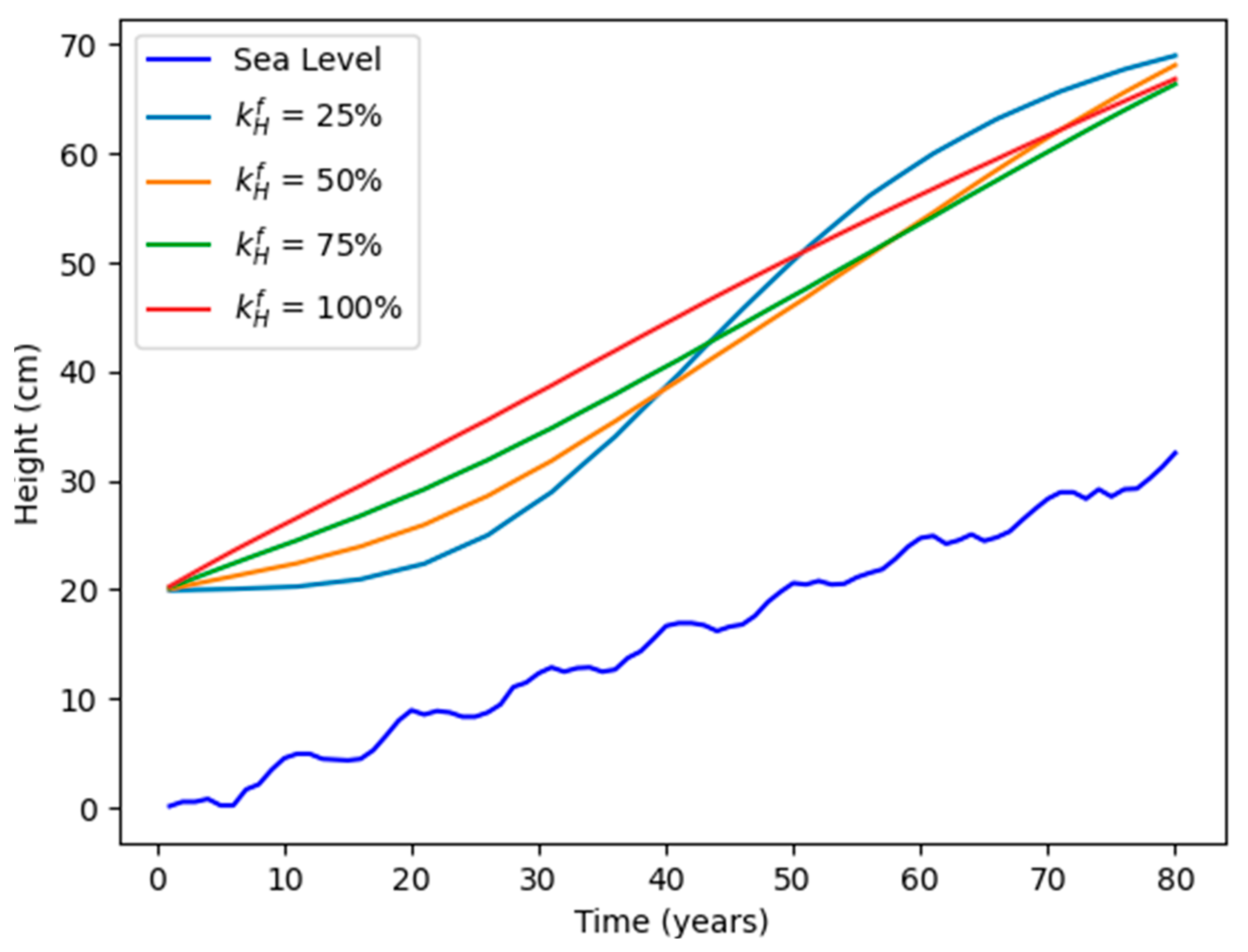
To investigate the effect of varying the fractional efficiency of coastal defense heightening on agent adaptation action, we carry out a sensitivity analysis for this parameter, taking values of 25%, 50%, 75%, and 100% (at 0% efficiency, the agent cannot invest in defense heightening at all and effectively cannot act). As described above, fractional efficiency represents inefficiencies in governance and adaptation plan implementation and is heavily system-dependent.
From the agent response curves in
Figure A1, we observe that at 25% efficiency, the agent takes much longer to adapt to rising sea levels and overshoots the optimal defense height due to slower plan implementation. The speed of agent response increases with increasing efficiency until 100%, where the agent’s averaged response is completely linear, following the gradual sea-level rise.
Figure A1.
Averaged coastal defense height for varying values of fractional efficiency of coastal defense heightening.
Figure A1.
Averaged coastal defense height for varying values of fractional efficiency of coastal defense heightening.
Appendix B
At every timestep, the optimizing agent has to calculate the optimal value V*, which will represent its target. We have defined the value of the agent as follows:
where utility U and disutility W are given by:
where
, and income obtained from the city Y = capital K, and
is a parameter describing the relative importance of negative utility with respect to positive utility.
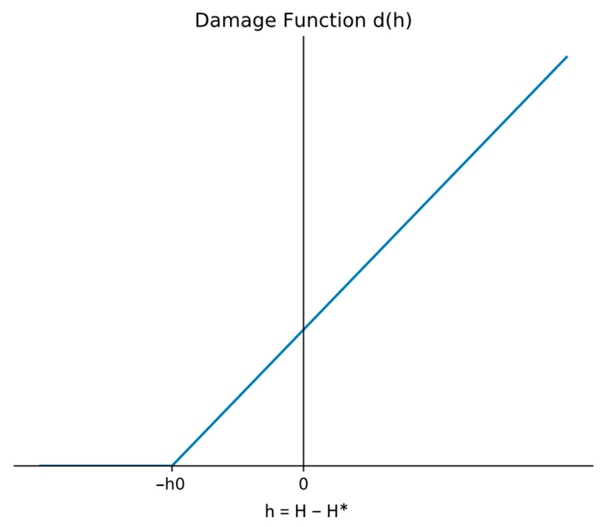
The damage function is taken as:
From the state dynamics equations, at the end of every timestep:
Substituting these in the damage function, the value equation becomes:
To obtain a linearly increasing function for d that starts rising after the value of excess height
crosses a threshold value h
0 > 0, we take it as a piecewise function defined as:
where h
s > 0.
Taking
, the value equation in terms of C
H and C
R becomes:
where θ is a step function defined as:
We make a few substitutions for brevity:
This reduces the value equation to:
With the constraint that
.
In addition, whenever , the optimal total investment amount would be zero, so we can take as another constraint.
To find an analytical solution for V*, we introduce:
Defining the value equation in terms of these new parameters:
In this equation, when , the disutility term disappears, leaving value dependent decreasingly on , i.e., , so for maximizing, we impose the constraint that .
So, we have the following boundary constraints:
Staying within the domain bound at
,
,
, and
(
Figure A2), we can vary a parameter
such that
. Thus, keeping
constant, we find that the minimum value of V is reached at
, and increases towards the edges of the domain. Thus, we can infer that the maximum value of V is reached at the boundary of this domain. Applying this to both
and
, we can see that V is maximized when either
or
.
Figure A2.
Boundary constraints on and .
Figure A2.
Boundary constraints on and .
To find a solution analytically, we assume
:
Since only the boundary conditions result in a maximization, either or holds true (in both cases, the other parameter is variable).
To maximize the above, we consider an auxiliary function f defined as:
where q > 0 and x lies between the bounds x
min and x
max. f(x) has an extremum point at x
0 where:
Thus, the maximum value of f(x) is reached at xmin, xmax, or x0. The terms f(xmin), f(xmax), and f(x0) would have to be computed, and the corresponding value of x would therefore be the target value.
So, to maximize , we use the following algorithm:
The above algorithm yields target values
and
, which are used to calculate C* and r* as follows:
Appendix B.1. Special Case for α and β
To take a more generalized scenario, we can prescribe that utility increases linearly and disutility changes at an arbitrary rate > 0, i.e., and .
We start with the value equation as computed earlier, this time substituting
instead:
where β is an arbitrary positive value.
We take a similar auxiliary function:
As a result, the same algorithm is followed, with only the terms
and
calculated in Steps 2 and 4, respectively, being changed:
where
and
.
The rest of the algorithm remains unchanged.


