Article

On a Data-Driven Optimization Approach to the PID-Based Algorithmic Trading

by
Vadim Azhmyakov
1,*,†,
Ilya Shirokov
2,†,
Yuri Dernov
2,† and
Luz Adriana Guzman Trujillo
3,†
1
Data Analytics, Universidad Central, Bogota 11001, Colombia
2
Algorithmic Systems Corp, Phuket 83000, Thailand
3
LARIS, Université d’Angers, 49000 Angers, France
*
Author to whom correspondence should be addressed.
These authors contributed equally to this work.
J. Risk Financial Manag. 2023, 16(9), 387; https://doi.org/10.3390/jrfm16090387
Submission received: 28 April 2023 / Revised: 3 August 2023 / Accepted: 7 August 2023 / Published: 30 August 2023
(This article belongs to the Section Mathematics and Finance)

Abstract

:
This paper proposes an optimal trading algorithm based on a novel application of conventional control engineering (CE). We consider a fundamental CE concept, namely, the feedback control, and apply it to algorithmic trading (AT). The concrete feedback control strategy is designed in a form of the celebrated proportional–integral–derivative (PID) model. The highly fluctuating nature of the modern financial markets has led to the adoption of a model-free realization of the generic PID framework. The control theoretical methodology we propose is combined with the advanced statistics for the historical market data. We obtain a specific log-normal probability distribution function (pdf) associated with the specific quantities associated with the available stock data. The empirical log-normal pdf mentioned above enables the necessary PID gains optimization. For this aim, we apply the data-driven optimization approaches and consider the corresponding Monte Carlo solution procedure. The optimized PID trading algorithm we propose is also studied in the Fourier analysis framework. This equivalent frequency domain representation involves a new concept in financial engineering, namely, the “stock market energy” concept. For the evaluation, we implement the proposed PID optimal trading algorithm and develop a Python-based prototype software. We finally apply the corresponding prototype software to a data set from the Binance BTC/USDT (Bitcoin/Tether) stock market. The experimental result illustrates the implementability of the proposed optimal PID trading scheme and also shows the effectiveness of the proposed CE methods in the modern AT.

1. Introduction and Motivation

The optimal design of profitable trading algorithms for financial markets constitutes a very challenging and technically sophisticated problem ofthe modern financial engineering (see Azhmyakov et al. 2021, 2022a, 2022b; Barmish 2008; Barmish and Primbs 2012, 2016; Baumann 2017; Bemporad et al. 2010; Malekpour et al. 2013; Rudoy and Rohrs 2008; Vo and Ślepaczuk 2022). It is well known that the highly fluctuating stock market prices and the corresponding highly frequent changes in the main market indicators make accurate forecasting nearly impossible. The same is also true with respect to forecasting-based optimization and trading. In a number of recent papers, a new line of research was developed which is aimed at using the feedback concepts from the modern CE in a model-free stock trading context. We refer to Azhmyakov et al. (2022a); Barmish (2008); Barmish and Primbs (2012, 2016); Baumann (2017) for technical details and further references. In this paper, we extend the above feedback-based approach to the algorithmic trading and propose some optimization procedures for the PID trading.
In order to develop the PID optimal trading algorithm, we consider an idealized stock market characterized by some specific technical assumptions. We examine a market under the assumption of “no transaction costs” and also consider “one stock portfolio”. We also introduce some further simplifying hypotheses, namely, the assumption of the “zero interest” and the so-called “continuous trading” conditions. Let us refer to Barmish (2008), Barmish and Primbs (2012, 2016) for the necessary technical details and existing abstractions in the modeling of the real-world stock markets. Our paper deals with the discrete-time dynamics of the financial markets under consideration. This assumption is motivated by the generic stock tick dynamics and also by the discrete-time decision-making process. Recall that a tick is a measurement of the minimum upward or downward movement in the price of a security (see, for example, Huang 2008; Michaud and Michaud 2008 and the references therein). The given discrete-time dynamics of the stock market ticks naturally implies a discrete-time process of the trading decision making. We next use the following notation of the stock ticks t = 1 , , and consider the corresponding semi-open time intervals of the trading buckets [ t , t + 1 ) . The market prices and all the additional market indicators (as volatility and other), as well as the trading decisions are related to the above stock ticks.
In this paper, we study the aforementioned idealized stock market and apply the CE-based PID control design to the development of an efficient trading algorithm. Recall that the PID control synthesis constitutes one of the most powerful and successful real-world control algorithms (see, for example, Azhmyakov 2019; Issidori 1995; Khalil 2015; Poznyak 2008; Prakash and Srinivasan 2009). The conventional model-based PID control implements a fundamental idea of the feedback control action and is widely used in various real-world engineering applications (see Azhmyakov 2019 and references therein). Our main idea is to extend the classic PID-based optimal control and decision techniques to a class of the model-free AT problems. The salient feature of this approach is that no model for stock price dynamics is used to determine the dollar amount invested. The investment level is performance-driven and generated in a model-free manner via an adaptive feedback on the cumulative return. Optimization of the current feedback parameters, namely, of the PID gains and the resulting trading algorithm structure, constitutes the novelty of our contribution and implies maximization of the cumulative return.
Advanced financial engineering and financial economics constitute a powerful theoretical tool of the modern financial science (see Black and Scholes 1973; Brooks 2015; Hens and Rieger 2010; Taylor 1986). On the other hand, the modern mathematically rigorous time-series-based financial theories cannot be directly applied to an algorithmic generation of the profitable trading decisions (see Azhmyakov et al. 2021, 2022a, 2022b; Barmish 2008; Barmish and Primbs 2012 and references therein). This fact is a simple consequence of the highly fluctuating stock prices. This fundamental property of the modern financial markets implies the so-called high-frequency trading (HFT) methodology. We refer to Brooks (2015) for the useful HFT concepts and some related technical details. A successful HFT strategy development is a very sophisticated and challenging task. In this paper, we propose to use some fundamental aspects of the conventional CE for this purpose. More specifically, we propose to apply an optimized PID type control strategy to the trading. This optimization technique involves some novel data-driven PID gains tuning approaches. The CE-based approach to the modern AT was originated in Barmish (2008); Barmish and Primbs (2012, 2016); Baumann (2017); Bemporad et al. (2010); Formentin et al. (2018); Malekpour et al. (2013). Let us also refer to Azhmyakov et al. (2021, 2022a) for some novel PID trading algorithms with a switched structure. The non-regular, highly frequent bid–ask spread behavior on a stock does not admit a realistic price-forecasting model. Hence, instead of modeling them, we propose to react to the stock price variations using the classic model-free PID control. We also combine the conventional PID trading with an advanced statistical characterization of the historical market data sets. We next identify a specific log-normal probability distribution function (pdf) for some concrete market quantities related to the data sets under consideration. Recall that a PID control design incorporates the important PID gains tuning procedure (see Azhmyakov 2019; Issidori 1995; Khalil 2015; Poznyak 2008). The established log-normal pdf for the market quantities mentioned above can next be used in an optimal PID gains tuning scheme.
Note that various optimization techniques play an important role in modern financial engineering (see, for example, Azhmyakov et al. 2022a, 2022b; Birge and Louveaux 2011; Hammel and Paul 2002; Jansen 2020; Lewis 1986; Liu and Wright 2015; Nemirovski et al. 2009; Wets 1990; Zenios 1993; Ziemba and Vickson 1975 and the references therein). In our case, we examine two different data-driven optimization approaches to the PID gains optimization, namely, the regression-based technique and the stochastic optimization framework. The first approach is combined with the well-known forward testing methodology Azhmyakov et al. (2022a); Zenios (1993). It considers the corresponding in-sample and out-of-sample concepts for a concrete data set. On the other hand, the classic stochastic optimization framework uses the established log-normal distribution of the introduced market quantities and leads to the celebrated Monte Carlo solution technique (see, for example, Hammel and Paul 2002; Shapiro and Homem-de-Mello 2000). The resulting PID trading algorithm with the optimized gains was applied to some concrete real-world examples. We consider a trading application on the Binance BTC/USDT spot market and illustrate the implementability, efficiency and profitability of the proposed algorithm. We also briefly discuss the prototype software for the proposed optimal PID trading algorithm.
The remainder of our paper is organized as follows: Section 2 contains a formal AT problem statement. This section includes a rigorous mathematical description of the conceptually novel model-free PID trading algorithm. In Section 3, we perform an advanced statistical analysis of the stock market data. We establish the log-normal probability distribution properties for some specific subsequential market characteristics. Section 4 deals with the main problem of the PID trading, namely, with the optimal PID gains tuning. We consider the data-driven optimization associated with the historical data and the corresponding backtesting procedure. The generic regression analysis is next applied in the general forward testing framework. In this section, we also propose an alternative PID gains selection strategy and use a scenario-based stochastic optimization problem for this purpose. The resulting stochastic program is solved by the Monte Carlo approach. In Section 5, we discuss a novel Fourier-based frequency domain interpretation of the proposed PID trading strategy. We apply the conventional z-transformation for the constructive characterization of the PID trading scheme in the frequency domain. Section 6 contains a practically motivated application of the developed PID trading algorithm to a specific stock market, namely, the Binance BTC/USDT futures stock. This section is also devoted to the prototype software design. Section 7 summarizes our paper.

2. Model-Free PID-Based Trading Algorithm

This section formally describes a novel concept of the model-free PID trading algorithm. Consider trading on an idealized stock market mentioned above. Let I ( 1 ) = I 1 be an initial deposit (initial investment). We next introduce the current return
Δ g ( t ) , t = 1 , , .
The current investment level at a time instant t is denoted by Δ I ( t ) . In parallel with the current values introduced above, we also consider the cumulative return and the cumulative investment g ( t ) and I ( t ) , respectively. The nonlinear discrete-time PID trading strategy can be formalized as follows:
δ I ( t + 1 ) = K P ( t + 1 ) Δ g ( t ) + K D ( t + 1 ) Δ ˙ g ( t ) + K I ( t + 1 ) t T t h ( τ ) Δ g ( τ ) d τ , Δ I ( t + 1 ) = χ ( δ I ( t + 1 ) ) , for t = 1 , .
By K P ( · ) , K D ( · ) and K I ( · ) , we denote here the necessary PID gains for the proportional, derivative and integral terms of the classic PID regulator scheme (see Azhmyakov 2019; Issidori 1995; Khalil 2015). Let us introduce the vector of these PID gains:
K ( · ) : = ( K P ( · ) , K D ( · ) , K I ( · ) ) T .
Note that the integral term in (1) incorporates the “process memory” on a given time interval [ t T , t ] . The integral kernel h ( · ) in (1) is defined by a suitable “memory loss” function h ( · ) . We consider here a simple exponential function h ( · ) with h ( t ) = 1 . Note that the proposed scheme (1) is similar to the classic PID control design (see, for example, Khalil 2015; Poznyak 2008). The nonlinear function χ ( · ) in (1) constitutes a specific “control saturation” and can be defined as follows:
χ ( δ I ) : = δ I , if δ I min | δ I | δ I max ; ± δ I max , if | δ I | > δ I max ; 0 , if | δ I | < δ I min .
Here δ I max , δ I min are prescribed as the maximal and minimal current investment levels, respectively. The above “saturated” investment model constitutes a formal mathematical condition and serves as a natural restriction for the investment volume.
Assuming the investment decision Δ I ( t + 1 ) in (2) and taking into consideration the stock price p ( ω , t + 1 ) , we next calculate the current return g ( t + 1 ) :
Δ g ( t + 1 ) = ( p ( · , t + 1 ) p ( · , t ) ) p ( · , t ) Δ I ( t + 1 )
If we use the CE analogy, we conclude that the proposed investment level Δ I ( t + 1 ) in (1) plays the role of a “control input”. Note that the current investment decision Δ I ( t + 1 ) is deployed at a present time instant t under the condition of a natural unknownness of the market price
p ( ω , t + 1 )
to the subsequent time instant ( t + 1 ) . By ω Ω and Ω , we denote here a probability state space with an unknown probability measure. The stock price
p : Ω × Z + R
is assumed to be a measurable stochastic function. Note that the current return Δ g ( t + 1 ) is a calculated a posteriori value, where p ( · , t + 1 ) in (3) denotes a concrete realization of the stochastic price p ( ω , t + 1 ) .
Since we have a clear CE analogy, we also can represent the above PID trading algorithm (1)–(3) using the corresponding block diagram. The corresponding block scheme of the proposed model-free PID trading strategy (1)–(3) is presented in Figure 1.
Note that the feedback channel in (1)–(3) is implemented by the current return Δ g ( t + 1 ) in (3). In fact, the PID trading algorithm (1)–(3) and the corresponding block diagram (Figure 1) represent the so-called “delayed PID” scheme. We refer to Khalil (2015) for details.
The general integral formula for δ I ( t + 1 ) in (1) can be rewritten in discrete time:
δ I ( t + 1 ) = ( K P ( t + 1 ) + K I ( t + 1 ) + K D ( t + 1 ) ) Δ g ( t ) + ( K I ( t + 1 ) h ( t 1 ) K D ( t + 1 ) ) Δ g ( t 1 ) + K I ( t + 1 ) τ = t T t 2 h ( τ ) Δ g ( τ ) .
Recall that the main CE problem of the conventional PID control approach consists in defining an adequate PID gains tuning rule (see, for example, Issidori 1995; Khalil 2015 and the references therein). In the generic real-world application fields of the classic PID controllers, the tuning techniques are well established Azhmyakov (2019); Poznyak (2008). For the conceptually new model-free PID algorithm under consideration, an adequate design of the PID gains tuning schemes constitutes a challenging problem. The suitable PID gains selection strategy immediately determines the trading decision signal by the proposed rule (4). In fact, the development of an adequate (optimal) PID gains tuning scheme constitutes a key problem for the profitable PID-based investment decision.
Let us also note that the model-free character of the proposed PID scheme (1)–(3) and (4) indicates the possibility to apply some suitable machine learning (ML) approaches to the corresponding optimal PID gains tuning problem. We refer to Bertsekas (2019); Bertsimas and Lo (1998); Jansen (2020) for the technical details related to the reinforcement learning (RL) approach and to some applications of the ML techniques in the modern AT.

3. Statistical Assumptions on the Stock Market

This section introduces some specific subsequential market characteristics and describes our discovery of the concrete probability distribution functions associated with these new quantities. We study here the PID gains tuning problem and use the obtained statistical information related to the stock market. Let us introduce the following “price/volume” ratio:
θ ( ω , t + 1 ) : = p ( ω , t + 1 ) v ( t + 1 ) .
Here, p ( ω , t + 1 ) is an unknown (stochastic) price at the time instant t + 1 and v ( t + 1 ) is an investment volume at the same time instant:
v ( t + 1 ) : = Δ I ( t + 1 ) p ( · , t ) .
Note that (6) expresses the entities number of a traded financial instrument (for example, futures trading). The comprehensive (a posteriori) statistical analysis of a wide spectrum of stock instruments demonstrates that the pdf of the above value θ ( ω , t ) constitutes a specific log-normal distribution (see, for example, Crow and Shimizu 1988; Gallager 2013; Poznyak 2009; Ziemba and Vickson 1975 and the references therein). Clearly, the real investment volumes of a hedge fund, a private trader or a bank are usually restricted. In the case of the PID trading algorithm (1)–(3), the maximal investment volume is formalized by the bound of Δ I ( t + 1 ) in (1) and (6).
The log-normal pdf related to the financial markets has mainly been studied for option prices. In this connection, we also refer to the celebrated Black and Scholes model Black and Scholes (1973). A useful discussion on this subject can also be found in Taylor (1986). Let us also mention the empirical log-normal pdf for some volatility-involved quotients and other stock market indicators (see, for example, Antoniou et al. 2004; Azhmyakov et al. 2022b; Crow and Shimizu 1988; Hens and Rieger 2010). We next analyze the stationary statistical distribution ρ 1 ( · ) of the quantity θ ( ω , t + 1 ) from (5):
ρ 1 ( θ ) = 1 2 π σ ( θ s ) exp ( ln ( θ s ) μ ) 2 ( 2 σ 2 ) ,
where θ > s 0 . Here, μ R denotes a statistical mean, σ R + is a dispersion and s R denotes a shifting. Note that (7) is often called a “three-parameter”
{ μ , σ , s }
log-normal distribution (see, for example, Antoniou et al. 2004; Crow and Shimizu 1988). The concrete parameter values of the log-normal pdf ρ ( θ ) can be calculated using the backtesting on the historical stock market data. As mentioned above, (7) constitutes an adequate model distribution for the introduced price/volume ratio θ ( ω , t + 1 ) . The quality of this statistic model can be established by application of the Chi-squared test for distribution qualification. We refer to Poznyak (2009) for the necessary technical details. For example, one can consider the normalized value χ 2 / q for the above test. Here, q is the number of degrees of freedom.
Note that the application of some exact statistical tests, for example, the Jarque–Bera test, constitutes a future work. This idea to implement an exact test and to establish whether the stock market data match a log-normal distribution can lead to very interesting research.
The concrete stock market histogram for a monthly Binance BTC/USDT price/volume ratio θ ( ω , t + 1 ) is depicted in Figure 2.
In parallel with (7), we also consider the log-normal pdf for the following price/price ratio:
ϑ ( ω , t + 1 ) : = p ( ω , t + 1 ) p ( · , t ) ,
where
{ p ( 1 ) , , p ( T ) } , { v ( 1 ) , , v ( T ) } .
are the stock prices and investment volumes data for the time instants t = 1 , , T . The log-normal probability distribution for the value ϑ ( ω , t + 1 ) in (8) was established in Antoniou et al. (2004). We denote this pdf by ρ 2 ( · ) . We also refer to Azhmyakov et al. (2022b); Brooks (2015) for the necessary statistical and econometric details.
We next obtain
ln ( θ ( ω , t + 1 ) / θ ( · , t ) ) = ln p ( ω , t + 1 ) p ( · , t ) ln v ( t + 1 ) v ( t ) .
and
ln v ( t + 1 ) v ( t ) = ln p ( ω , t + 1 ) p ( · , t ) + ln θ ( · , t ) ln θ ( ω , t + 1 ) .
Expressions (9) and (10) make it possible to generate a part of the complete investment decision, namely, the decision about the investment volume v ( t + 1 ) to the time instant t + 1 :
v ( t + 1 ) = exp [ ln p ( ω , t + 1 ) p ( · , t ) + ln θ ( · , t ) ln θ ( ω , t + 1 ) + ln v ( t ) ] .
Observe that θ ( · , t ) and v ( t ) in (11) are known values. Additionally, the price/volume ration θ ( ω , t + 1 ) and the price/price ratio
p ( ω , t + 1 ) p ( · , t )
can effectively be simulated using the corresponding log-normal probability distribution functions. We next can also forecast the value
ln p ( ω , t + 1 ) / p ( · , t )
in (11) using the corresponding log-normal distribution (see Antoniou et al. 2004; Azhmyakov et al. 2022b; Crow and Shimizu 1988). We assume here that the necessary parameters of the log-normal distributions of the values θ ( ω , t + 1 ) and
p ( ω , t + 1 ) / p ( · , t )
are previously determined by the generic backtesting technique. For example, for (7), we need to identify a , μ , σ , s . This identification procedure is performed using the available statistics in the form of a histogram (see, for example, Figure 2).
Assuming the investment volume decision (11), we immediately obtain a tuning scheme for the PID gains K ( · ) . Combining (6) and (11), we finally obtain
χ ( K P ( t + 1 ) Δ g ( t ) + K D ( t + 1 ) Δ ˙ g ( t ) + K I ( t + 1 ) t T t h ( τ ) Δ g ( τ ) d τ ) = p ( · , t ) exp [ ln p ( ω , t + 1 ) p ( · , t ) + ln θ ( · , t ) ln θ ( ω , t + 1 ) + ln v ( t ) ] .
Since the investment decision Δ I ( t + 1 ) is designed by the PID rule (1)–(2), the obtained formulae (12) constitute a specific tuning restriction for the PID gains K ( · ) . This novel tuning approach involves the advanced statistical (log-normal) analysis of the financial market behavior.

4. Data-Driven Optimization Approaches to the PID Gains Tuning

A credible anticipatory strategy for the behavior of stock markets (using a certain amount of historical data) constitutes the main conceptual problem of algorithmic trading. In the framework of the proposed PID trading algorithm (1)–(3), we have to incorporate into the PID methodology an additional optimization procedure for a “best choice” of the PID gains. In this section, we describe two advanced optimization approaches to the optimal PID gains tuning. The resulting PID-based strategies (1)–(3) with an optimal gain selection are next called optimal PID trading algorithms. Let us note that the “advanced” character of the optimal tuning mentioned above corresponds to the model-free structure of the proposed PID trading scheme. The model-free nature of an optimal PID implementation (1)–(3) also indicates the usability of the modern ML and RL approaches for optimal PID gains selection problems. Let us refer to Bertsekas (2019); Bertsimas and Lo (1998); Jansen (2020) for some technical results and novel ideas.

4.1. Regression Involved Gains Optimization

In this section, we use a conventional regression-based optimization framework applied to the historical stock data. Our aim is to combine the least square optimization with the generic forward testing (FT). Note that the FT technique is a common methodology of the modern AT (see, for example, Hens and Rieger 2010; Jansen 2020). It includes the so-called in-sample and out-of-sample data subsets of the initially given historical data set. The in-sample data set is part of historical data on which the optimization is performed. The subset of historical data that was reserved for a possible validation of the optimized trading algorithm is known as an out-of-sample data set.
We now choose a number M 1 N as a cardinal number of the in-sample set and consider the corresponding investment volumes:
v j ( t + 1 ) , j = 1 , , M 1 1 .
Let M 2 denote a cardinal number of the out-of-sample set such that the complete historical data set under consideration has
M : = M 1 + M 2
elements. Using the given (nonlinear) structure of the PID trading algorithm (1)–(3), we next introduce the following main optimization problem:
J 1 ( K ( t + 1 ) ) : = j = 1 M 1 ( χ ( δ I ( t + 1 ) ) v j ( t + 1 ) p ( · , t + 1 ) ) 2 min K ( t + 1 ) subject to ( 1 ) ( 3 ) , ( 12 )
Evidently, (13) constitutes a specific nonlinear regression determined on the in-sample data set. Note that problem (13) involves the previously obtained statistical characterization (12). This statistical result for the PID gains constitutes a natural restriction in the minimization problem (13). The main problem (13) can be solved by some known numerical optimization methods (see, for example, Azhmyakov et al. 2021; Gill et al. 1981; Lewis 1986 and the references therein). It finally leads to the optimal PID gains selection:
K o p t ( t + 1 ) : = { K P o p t ( t + 1 ) , K D o p t ( t + 1 ) , K I o p t ( t + 1 ) } .
The out-of-sample data set can next be used for the validation procedure of the optimal solution K ( t + 1 ) obtained using the in-sample set. This validation is based on the comparison of two values of the same objective functional from (13), namely, the in-sample optimal value
J 1 ( K o p t ( t + 1 ) )
and the following out-of-sample optimal value
J 2 ( K o p t ( t + 1 ) ) : = j = 1 M 2 ( χ ( δ I o p t ( t + 1 ) ) v j ( t + 1 ) p ( · , t + 1 ) ) 2 .
Note that the out-of-sample optimal investment
δ I o p t ( t + 1 ) )
in (14) is calculated using the optimal gains K o p t ( t + 1 ) (obtained on the in-sample data set) and the basic expression from (1). Moreover, the set of investment volumes v j ( t + 1 ) in (14) corresponds to the out-of-sample set:
v j ( t + 1 ) , j = 1 , , M 2 1 .
The above optimization problem (13) is considered a consistent (optimal) PID gains selection procedure if
| J 1 ( K o p t ( t + 1 ) ) J 2 ( K o p t ( t + 1 ) ) | ϵ
for a sufficiently small prescribed ϵ > 0 . Let us note that an alternative validation procedure for the PID gains optimization can involve the celebrated Monte Carlo approach (see, for example, Hammel and Paul 2002; Rubinstein and Kroese 1981).
We now apply the validated optimal gains vector
K o p t ( t + 1 )
for defining the deployed (optimal) investment level
Δ I o p t ( t + 1 )
using the PID algorithm (1)–(3). The resulting optimal investment volume
v o p t ( t + 1 )
for the time instant ( t + 1 ) has the following expression:
v o p t ( t + 1 ) : = Δ I o p t ( t + 1 ) p ( · , t + 1 ) .
Note that the complete trading decision at the time instant ( t + 1 ) generated by the proposed algorithm can be formalized using the following “trading signal/volume” pair:
{ trading signal , trading volume } : = { sign [ Δ I o p t ( t + 1 ) ] , | v o p t ( t + 1 ) | } .
Here, sign [ · ] is the signum function. Moreover,
trading signal : = sign [ Δ I o p t ( t + 1 ) ]
denotes the optimal trading signal and
trading volume : = | v o p t ( t + 1 ) |
is the absolute value of the optimal investment volume. The above trading signal/volume pair definitively determines a subsequent ( t + 1 ) -trading decision in the proposed PID trading framework. The nonlinear optimization approach (13) implies that the optimal investment decision
Δ I o p t ( t + 1 )
constitutes an a priori (optimal) value in the above trading signal/volume pair. The corresponding optimal volume v o p t ( t + 1 ) is in fact an a posteriori value for the subsequent time instant ( t + 1 ) .

4.2. On the Stochastic Optimal Gains Tuning

The optimal gains selection problem (13) from the previous section constitutes a data-driven regression-based approach. This generic optimization approach involves a constrained nonlinear optimization and uses the given historical stock market data. An additional FT technique discussed in the previous section constitutes in fact an adequate expert driven clustering of the complete historical data set. Note that this separation of the initially given data set is methodologically similar to the main idea of the celebrated Monte Carlo method (see Birge and Louveaux 2011; Hammel and Paul 2002; Rubinstein and Kroese 1981 and references therein). Let us recall that the classic Monte Carlo method also contains the so-called “training” and “validation” solution steps (see, for example, Birge and Louveaux 2011; Cornuejols et al. 2018; Wets 1990).
In this section, we will formulate the stochastic optimization problem for an adequate gains selection in the proposed PID trading framework (1)–(3). The stochastic programming problem we consider is conceptually different from the regression-like problem (13). It involves the specific statistical description of the stock markets obtained in Section 3. Using (11), we next introduce the following minimization problem:
J ( ω , K ( t + 1 ) ) : = j = 1 M ( χ ( δ I ( t + 1 ) ) exp [ ln p ( ω , t + 1 ) p ( · , t ) + ln θ ( · , t ) ln θ ( ω , t + 1 ) + ln v ( t ) ] × p ( ω , t + 1 ) ) 2 min K ( t + 1 ) subject to ( 1 ) ( 3 ) , ( 12 )
The above optimization problem constitutes a nonlinear stochastic program (see, for example, Birge and Louveaux 2011; Wets 1990). Clearly, problem (15) now contains a probabilistic functional cost
J ( ω , K ( t + 1 ) ) , ω Ω .
The stochastic program (15) can be interpreted as a two-stage or a multistage problem. We refer to Birge and Louveaux (2011); Michaud and Michaud (2008), for the necessary concepts of stochastic programming. However, we consider here the scenarios-based Monte Carlo optimization approach (see, for example, Birge and Louveaux 2011). In this section, we study this stochastic problem (15) only from a conceptual point of view and discuss the corresponding Monte Carlo sampling solution method.
Taking into consideration the mean value approach, we replace (15) by the following deterministic program:
J E ( K ( t + 1 ) ) : = j = 1 M E ρ 1 ( · ) , ρ 2 ( · ) ( χ ( δ I ( t + 1 ) ) exp [ ln p ( ω , t + 1 ) p ( · , t ) + ln θ ( · , t ) ln θ ( ω , t + 1 ) + ln v ( t ) ] × p ( ω , t + 1 ) ) 2 min K ( t + 1 ) subject to ( 1 ) ( 3 ) , χ ( K P ( t + 1 ) Δ g ( t ) + K D ( t + 1 ) Δ ˙ g ( t ) + K I ( t + 1 ) t T t h ( τ ) Δ g ( τ ) d τ ) = E ρ 1 ( · ) , ρ 2 ( · ) ( p ( · , t ) exp [ ln p ( ω , t + 1 ) p ( · , t ) + ln θ ( · , t ) ln θ ( ω , t + 1 ) + ln v ( t ) ] ) .
Here,
E ρ 1 ( · ) , ρ 2 ( · )
is the mathematical expectation operator with respect to the (joint) pdf for the pair
( θ ( ω , t ) , ϑ ( ω , t ) )
of quotients θ and ϑ introduced in Section 3. Note that the log-normal probability distribution functions ρ 1 ( · ) and ρ 2 ( · ) imply a statistical non-robustness of the mathematical expectation used in (16). The mean value optimization problem (16) does not possess the necessary robustness property (see Huber and Ronchetti 2005). This fact can cause deposit losses when problem (16) is directly used in the trading. In this situation, one can replace the mean value E ρ 1 ( · ) , ρ 2 ( · ) in problem (16) by a generic robust statistical characteristic (for example, the median and ctr.).
Let us also note that the auxiliary (deterministic) problem (16) constitutes a data-driven optimization. These minimization problems incorporate the empiric log-normal probability distribution functions ρ 1 ( · ) and ρ 2 ( · ) . This fact constitutes a methodological difference between the regression-based PID gains optimization (13) and (14) and the alternative PID tuning strategy based on the stochastic optimization problem (15).
The auxiliary problem (16) provides a possible approach to the numerical treatment of the initial problem (15). Following the Monte Carlo methodology, we define some probabilistic scenarios { ω i } , i = 1 , N with the corresponding probabilities
P ( ω = ω i ) , i = 1 , N
associated with the realizations of the stochastic variables (“stochastic events”)
Γ : = { ω 1 , , ω N } .
The celebrated scenarios-based approximating problem for (16) can now be formalized as follows:
J E ( K ( t + 1 ) ) : = j = 1 M i = 1 N P ( ω = ω i ) ( χ ( δ I ( t + 1 ) ) exp [ ln p ( ω i , t + 1 ) p ( · , t ) + ln θ ( · , t ) ln θ ( ω i , t + 1 ) + ln v ( t ) ] × p ( ω i , t + 1 ) ) 2 min K ( t + 1 ) subject to ( 1 ) ( 3 ) , χ ( K P ( t + 1 ) Δ g ( t ) + K D ( t + 1 ) Δ ˙ g ( t ) + K I ( t + 1 ) t T t h ( τ ) Δ g ( τ ) d τ ) = i = 1 N P ( ω = ω i ) ( p ( · , t ) exp [ ln p ( ω i , t + 1 ) p ( · , t ) + ln θ ( · , t ) ln θ ( ω i , t + 1 ) + ln v ( t ) ] ) .
Evidently, the finite sum in (17)
i = 1 N P ( ω = ω i ) g ( ω i , · )
approximates the mathematical expectation E ρ 1 ( · ) , ρ 2 ( · ) in the auxiliary problem (16).
Similar to the FT methodology used in the previous section, we now divide the above N-dimensional event set Γ into two subsets and define a suitable N 1 -dimensional training set and an additional N 2 -dimensional validation set
Γ 1 : = { ω 1 , , ω N 1 } , Γ 2 : = { ω 1 , , ω N 2 } .
Here,
N 1 + N 2 = N .
with
N N 1 .
The above division of the initially given N-dimensional scenarios set Γ makes it possible to consider the basic Monte Carlo approximating problem (17) on the training set Γ 1 and then on the full scenarios set Γ . In the case of an admissible mismatch in the values of the objective functionals of problem (17) considered on Γ 1 and on the full set Γ , the optimization procedure is successfully completed. Otherwise, one needs to increase the dimensionality of the historical data set and repeat the above training and validation steps in the Monte Carlo framework.
Let us note that in our paper, we do not consider the generic risk minimization problem. However, we propose a novel optimized PID trading algorithm. This algorithm possesses some adjustable parameters, namely, the vector functions of the gain coefficients. Optimization (maximization) of the cumulative return is performed with respect to the gain coefficients mentioned above. A resulting optimal vector of the gain coefficients involves a maximal return in the framework of the proposed PID trading algorithm. That means that the cumulative return maximization is a formal consequence of the specific optimization procedure (optimal tuning) applied to the gain coefficients.

5. Frequency Domain Representation of the PID Trading Algorithm

A formal frequency domain involved description of the feedback-based trading approach can be found in Azhmyakov et al. (2022a). Let us recall that the Fourier transform and the corresponding frequency domain analysis constitute a generic methodology in the classic CE. We refer to Poznyak (2008) for the corresponding mathematical foundations and some computational details of the Laplace and Fourier transforms in the CE framework.
In this section, we discuss the frequency domain analysis of the proposed PID trading algorithm (1)–(3). Let us also observe that the above PID trading algorithm can be interpreted as a specific control design with the time delays. Taking into consideration the main profit formulae (3), the linear expression δ I ( t + 1 ) in (1) can also be considered as an ARMA-like formal model. Note that the main expression for Δ I ( t + 1 ) in the PID formulae (1) constitutes, in fact, a nonlinear ARMA process. Let us also observe that the discrete time PID control (4) can also be considered a delayed proportional control.
We next apply the celebrated discrete signal processing (DSP) approach and interpret the linear expression for δ I ( t + 1 ) in (1) as a linear filter. Application of the z-transform to the discrete PID (4) implies the following generic form of the causal discrete-time finite impulsive response (FIR) filter (see Poznyak 2009):
Y ( z ) = ( K P ( s + 1 ) + K I ( s + 1 ) + K D ( s + 1 ) ) z + [ ( K I ( s + 1 ) h ( s ) K D ( s + 1 ) ) z 1 + K I ( s + 1 ) h ( s 1 ) z 2 + K I ( s + 1 ) τ = s T s 2 h ( τ ) z τ ] .
Here, Y ( · ) denotes the resulting z-transform of the initially given output signal
δ I ( t + 1 ) .
Note that z is the proper variable in (18). We next can easily obtain the frequency response function for the above FIR filter (18). Recall that frequency response of the filter (18) is a result of a the formal application of the DTFT (discrete time Fourier transform) to the FIR (18). Following Poznyak (2009), we next put
z exp ( j ω ) ,
where j in (18) denotes the imaginary unit. The frequency response F R ( · ) of the PID trading algorithm (1)–(3) can now be written as follows:
F R ( f ) = ( K P ( s + 1 ) + K I ( s + 1 ) + K D ( s + 1 ) ) × exp ( j f ) + [ ( K I ( s + 1 ) h ( s ) K D ( s + 1 ) ) × exp ( j f ) + K I ( s + 1 ) h ( s 1 ) × exp ( 2 j f ) + K I ( s + 1 ) τ = s T s 2 h ( τ ) × exp ( τ j f ) ] .
Here, f denotes the frequency of a dynamic process under consideration. Note that the obtained expression (19) for the proposed PID trading algorithm makes it possible to apply the well-developed frequency domain methodology to the PID gains tuning problem. The historical stock market data can be used here for an optimal selection of the above PID gains. Note that a practical calculation of a DTFT is usually performed by the so-called fast Fourier transform (FFT). This fact is motivated by a considerable number of the efficient FFT codes in the main programming languages.
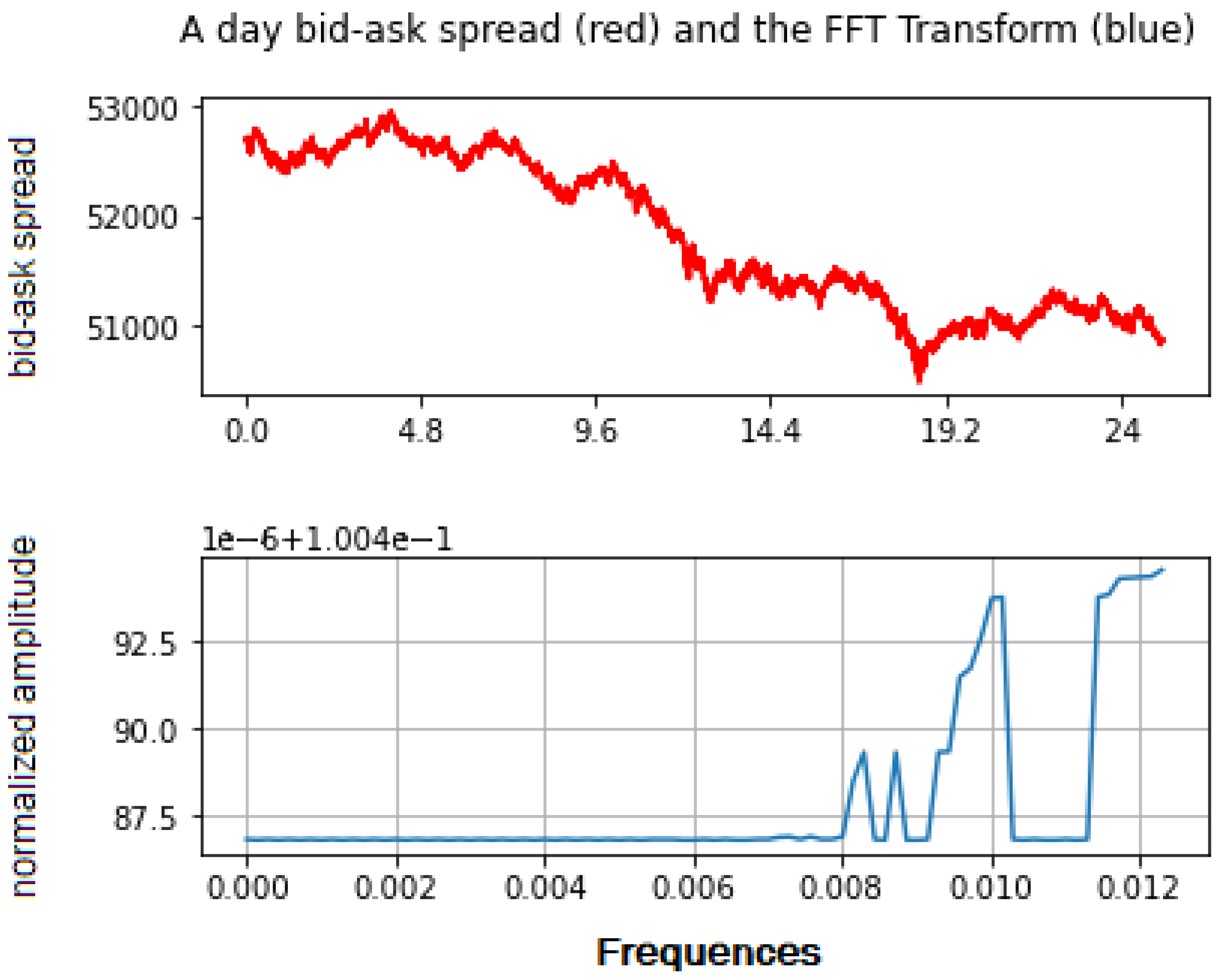
Let us give an illustrative computational example of the function F R ( · ) . Consider the one-day bid–ask spread dynamics of the Binance BTC/USDT exchange and its DTFT (Figure 3).
In fact, the resulting frequency diagram, namely, Figure 3 represents a specific “market energy” distribution associated with the corresponding price frequencies. This energetic interpretation of the resulting DTFT is related to the fundamental Parseval theorem from the classic Fourier analysis (see, for example, Poznyak 2009). Motivated by this consideration, we introduce the following market energy concept:
E : = i = 1 N F R 2 ( f ) ,
where N is the dimension of a one-day data set under consideration and F R ( f ) is the corresponding frequency response associated with this data set.
The developed optimal PID trading algorithm (1)–(3) can also be combined with several well-known momentum (trading) strategies (see, for example, Malekpour et al. 2013; Michaud and Michaud 2008). For example, a suitable trend following algorithm provides a future promising tool for an optimal frequency response-based PID gains selection procedure. In fact, the frequency domain analysis and the above market energy concept constitute a natural analytic tool for the HFT algorithmic trading. Finally note that the DTFT naturally represents the frequent character of the market prices and can be used as a new volatility indicator (in parallel with the well-known ATR volatility measure).

6. On the Implementation of the Optimal PID Trading Algorithm

We now present an application of the developed PID-based AT technique to real-world stock market data. Consider the Binance Bitcoin/USDT futures stock and apply the proposed optimal PID trading algorithm (1)–(3). The example of the one-day BTC/USDT futures bid–ask spread dynamics is presented in Figure 4.
We applied the developed PID trading algorithm with the optimized gains to the above one-day price market dynamics. The PID gains optimal tuning procedure for this example was performed using the data-driven optimization discussed in Section 4.1. The corresponding (globally positive) dynamics of the corresponding return is presented in Figure 5.
Note that the operation time for every subsequent trading decision of the resulting optimal PID in this example is time restricted. The stock market under consideration has an obvious high-frequency behavior. This fact naturally implies some expected difficulties of the common trading algorithms. In particular, this concerns the widely used moving average trading and the general trend following trading strategies.
As one can see, the proposed optimal PID constitutes an adequate strategy for the HFT. The time ticks in the stock example under consideration are significantly dense. The length of the corresponding intervals of trading buckets is equal to 1.728 s.
Let us also observe the generic “hyperregulation and stabilization” dynamics of the resulting PID trading algorithm with optimized gains (see Figure 5). This stabilizing dynamics is a characteristic behavior for the conventional PID controller. We refer to Azhmyakov et al. (2021); Issidori (1995); Khalil (2015); Poznyak (2008) for the corresponding examples and further technical details.
The presented practical example illustrates the implementability and effectiveness of the developed PID trading framework. As we can see, the resulting dynamics of the return constitutes profitable financial behavior. Let us also note that the dynamics of the BTC/USDT futures considered in this section constitute an admissible and adequate example of a financial market. It was used here as an initial illustration of the effectiveness and profitability of the proposed trading algorithm.

7. Concluding Remarks

In this paper, we developed a novel trading algorithm based on the model-free PID control methodology and some advanced statistical characteristics of the stock market. We considered an idealized financial market under the assumption of only one asset. However, the proposed analytic approach and the resulting trading methodology can naturally be extended to the real-time multi-asset trading. It can also be combined with some classical trading strategies (momentum strategies).
The main idea of the proposed PID control approach to the algorithmic trading consists of the modern data involved optimization techniques for the PID gains tuning. These data-driven optimization procedures determine an optimal “calibration” (tuning) of the main PID trading parameters. The resulting optimal PID gains finally define the subsequent trading decision (trading signal and trading volume). The optimization procedures we applied involve the conventional FT techniques and the regression analysis. The tuning procedure also involves the backtesting technique. We also shortly discussed a possible application of the classic stochastic optimization and Monte Carlo method in the framework of the optimal PID algorithm.
The given historical stock market data, the statistical properties mentioned above and the data-driven optimization of the PID gains are applied to a practical stock example. The resulting optimal trading PID strategy generates a profitable investment decision of the “buy/sell/hold” type for the stock market orders. The proposed CE-based approach to the modern AT involves a combination of some known mathematically rigorous tools. We use the classic feedback control methodology, applied statistics and computational optimization. The model-free character of the proposed PID trading scheme clearly indicates the possibility to apply some modern ML approaches to the PID trading algorithm design (see Bertsekas 2019; Bertsimas and Lo 1998; Jansen 2020). We also expect a profitable behavior of this trading methodology in terms of high-frequency trading.
Note that the developed PID-based trading approach can also be involved (as an additional tool) in several theoretic concepts of modern financial engineering. For example, it can be studied in the framework of the well-established financial time-series analysis and Kalman filter techniques (see, for example, Azhmyakov et al. 2021; Bahmani-Oskooee and Brown 2004; Lewis 1986). The proposed PID trading algorithm is also compatible with the possible price prediction and trend following techniques (see Huang 2008).
The algorithmic trading strategy proposed in our paper constitutes an initial theoretical development. We are mostly concentrated here on the mathematical and algorithmic aspects of the proposed technique. A necessary comparative analysis of the proposed optimal PID trading algorithm constitutes a further important topic. However, a suitable comparative study requires an extra journal paper. An adequate comparison mentioned above includes some comprehensive computational experiments and simulations. Moreover, the efficiency of the trading algorithm also depends on the concrete financial market and some additional trading parameters (trading volumes and so on). We define this challenging comparative research topic as a future work.
Finally, note that the prototypes of the financial solutions for the stock market proposed in our contribution need comprehensive computational development, additional simulations, prototyping and further backtesting on real stock market data.

Author Contributions

Conceptualization, V.A.; Methodology, L.A.G.T.; Software, Y.D.; Validation, I.S.; Formal analysis, I.S.; Investigation, L.A.G.T.; Data curation, L.A.G.T.; Writing—review & editing, V.A. All authors have read and agreed to the published version of the manuscript.

Funding

This research received no external funding.

Data Availability Statement

No new data were created.

Conflicts of Interest

The authors declare no conflict of interest.

References

  1. Antoniou, Ioannis E., Vi V. Ivanov, Va V. Ivanov, and Petr V. Zrelov. 2004. On the log-normal distribution of stock market data. Physica A 331: 617–38. [Google Scholar] [CrossRef]
  2. Azhmyakov, Vadim. 2019. A Relaxation Based Approach to Optimal Control of Switched Systems. Oxford: Elsevier. [Google Scholar]
  3. Azhmyakov, Vadim, Ilya Shirokov, and Luz Adriana Guzman Trujillo. 2022a. Application of a switched PIDD control strategy to the model-free algorithmic trading. IFAC PapersOnline 55: 145–50. [Google Scholar] [CrossRef]
  4. Azhmyakov, Vadim, Ilya Shirokov, Yuri Dernov, and Luz Adriana Guzman Trujillo. 2022b. On the Proportional-Integral-Derivative based trading algorithm under the condition of the log-normal distribution of stock market data. Paper presented at the Sixteenth International Conference on Advanced Engineering Computing and Applications in Sciences (ADVCOMP 2022), Valencia, Spain, November 13–17; pp. 17–21. [Google Scholar]
  5. Azhmyakov, Vadim, Jose Perea Arango, Moises Bonilla, Raymundo Juarez del Toro, and Stefan Pickl. 2021. Robust state Estimations in Controlled ARMA Processes with the Non-Gaussian Noises: Applications to the Delayed Dynamics. IFAC PapersOnline 54: 334–39. [Google Scholar] [CrossRef]
  6. Bahmani-Oskooee, Mohsen, and Ford Brown. 2004. Kalman Filter approach to estimate the demand for international reserves. Applied Economics 36: 1655–68. [Google Scholar] [CrossRef]
  7. Barmish, B. Ross. 2008. On trading of equities: A robust control paradigm. IFAC Proceedings Volumes 41: 1621–26. [Google Scholar] [CrossRef]
  8. Barmish, B. Ross, and James A. Primbs. 2012. On market-neutral stock trading arbitrage via linear feedback. Paper presented at the American Control Conference, Montreal, QC, Canada, June 27–29; pp. 3693–98. [Google Scholar]
  9. Barmish, B. Ross, and James A. Primbs. 2016. On a new paradigm for stock trading via a model-free feedback controller. IEEE Transactions on Automatic Control 61: 662–76. [Google Scholar] [CrossRef]
  10. Baumann, Michael Heinrich. 2017. On stock trading via feedback control when underlying stock returns are discontinuous. IEEE Transactions on Automatic Control 62: 2987–92. [Google Scholar] [CrossRef]
  11. Bemporad, Alberto, Tommaso Gabbriellini, Laura Puglia, and Leonardo Bellucci. 2010. Scenario-based stochastic model predictive control for dynamic option hedging. Paper presented at the IEEE Conference on Decision and Control, Atlanta, GA, USA, December 15–17; pp. 3216–21. [Google Scholar]
  12. Bertsekas, Dimitri. 2019. Reinforcement Learning and Optimal Control. Nashua: Athena Scientific. [Google Scholar]
  13. Bertsimas, Dimitris, and Andrew W. Lo. 1998. Optimal control of execution costs. Journal of Financial Markets 1: 1–50. [Google Scholar] [CrossRef]
  14. Birge, John R., and Francois Louveaux. 2011. Introduction to Stochastic Programming. New York: Springer. [Google Scholar]
  15. Black, Fischer, and Myron Scholes. 1973. The pricing of options and corporate liabilities. Journal of Political Economy 81: 637–59. [Google Scholar] [CrossRef]
  16. Brooks, Chris. 2015. Introductory Econometcs for Finance. Glasgow: Cambridge University Press. [Google Scholar]
  17. Cornuejols, Gérard, Pena Javier, and Tutuncu Reha. 2018. Optimization Methods in Finance. Cambridge: Cambridge University Press. [Google Scholar]
  18. Crow, Edwin L., and Kunio Shimizu, eds. 1988. Lognormal Distributions, Theory and Applications. New York: Marcel Dekker, Inc. [Google Scholar]
  19. Formentin, Simone, Fabio Previdi, Gabriele Maroni, and Claudio Cantaro. 2018. Stock trading via feedback control: An extremum seeking approach. Paper presented at the Mediterranean Conference on Control and Automation, Zadar, Croatia, June 19–22; pp. 523–28. [Google Scholar]
  20. Gallager, Robert G. 2013. Stochastic Processes. New York: Cambridge University Press. [Google Scholar]
  21. Gill, Philip E., Walter Murray, and Margaret H. Wright. 1981. Practical Optimization. New York: Academic Press. [Google Scholar]
  22. Hammel, C., and Wolfgang B. Paul. 2002. Monte Carlo simulations of a trader-based market model. Physica A 313: 640–50. [Google Scholar] [CrossRef]
  23. Hens, Thorsten, and Marc Oliver Rieger. 2010. Financial Economics. Berlin: Springer. [Google Scholar]
  24. Huang, Shian-Chang. 2008. Online option price forecasting by using unscented Kalman filters and support vector machines. Journal of Expert Systems with Applications 34: 2819–25. [Google Scholar] [CrossRef]
  25. Huber, P. J., and Elvezio Ronchetti. 2005. Robust Statistics. New York: Wiley. [Google Scholar]
  26. Isidori, Alberto. 1995. Nonlinear Control Systems. London: Springer. [Google Scholar]
  27. Jansen, Stefan. 2020. Machine Learning for Algorithmic Trading. Birmingham: Packt Publishing Ltd. [Google Scholar]
  28. Khalil, Hassan. 2015. Nonlinear Control. Boston: Pearson. [Google Scholar]
  29. Lewis, Frank L. 1986. Optimal Estimation. New York: Wiley. [Google Scholar]
  30. Liu, Ji, and Stephen J. Wright. 2015. Asynchronous stochastic coordinate descent: Parallelism and convergence properties. SIAM Journal on Optimization 25: 351–76. [Google Scholar] [CrossRef]
  31. Malekpour, Shirzad, James A. Primbs, and B. Ross Barmish. 2013. On stock trading using a PI controller in an idealized market: The robust positive expectation property. Paper presented at the IEEE Conference on Decision and Control, Florence, Italy, December 10–13; pp. 1210–16. [Google Scholar]
  32. Michaud, Richard O., and Robert O. Michaud. 2008. Efficient Asset Management. Oxford: Oxford University Press. [Google Scholar]
  33. Nemirovski, Arkadi, Anatoli Juditsky, Guanghui Lan, and Alexander Shapiro. 2009. Robust stochastic approximation approach to stochastic programming. SIAM Journal on Optimization 19: 1574–609. [Google Scholar] [CrossRef]
  34. Poznyak, Alexander S. 2008. Advanced Mathematical Tools for Automatic Control Engineers: Deterministic Technique. New York: Elsevier. [Google Scholar]
  35. Poznyak, Alexander S. 2009. Advanced Mathematical Tools for Automatic Control Engineers: Stochastic Tools. New York: Elsevier. [Google Scholar]
  36. Prakash, Jagadeesan, and K. Srinivasan. 2009. Design of nonlinear PID controller and nonlinear model predictive controller for a continuous stirred tank reactor. ISA Transactions 48: 273–82. [Google Scholar] [CrossRef] [PubMed]
  37. Rubinstein, Reuven Y., and Dirk P. Kroese. 1981. Simulation and the Monte Carlo Method. New York: John Wiley Inc. [Google Scholar]
  38. Rudoy, Melanie B., and Charles E. Rohrs. 2008. A dynamic programming approach to two-stage mean-variance portfolio selection in cointegrated vector autoregressive systems. Paper presented at the IEEE Conference on Decision and Control, Cancun, Mexico, December 9–11; pp. 4280–85. [Google Scholar]
  39. Shapiro, Alexander, and Tito Homem-de-Mello. 2000. On the rate of convergence of optimal solutions of Monte Carlo approximations of stochastic programs. SIAM Journal on Optimization 11: 70–86. [Google Scholar] [CrossRef]
  40. Taylor, Stephen J. 1986. Modeling Financial Time Series. Chichester: Wiley. [Google Scholar]
  41. Vo, Nguyen, and Robert Ślepaczuk. 2022. Applying hybrid ARIMA-SGARCH in algorithmic investment strategies on S&P500 index. Entropy 24: 158. [Google Scholar] [CrossRef] [PubMed]
  42. Wets, Roger J.-B. 1990. Stochastic programming. In Optimization, Handbooks in Operations Research and Management Science. Edited by Nemhauser George L., Rinnooy Kan A. H. G. and Todd Michael J. New York: Elsevier, vol. 1. [Google Scholar]
  43. Zenios, Stavros A., ed. 1993. Financial Optimization. Cambridge: Cambridge University Press. [Google Scholar]
  44. Ziembaand, William T., and Raymond G. Vickson. 1975. Stochastic Optimization Models in Finance. New York: Academic Press. [Google Scholar]
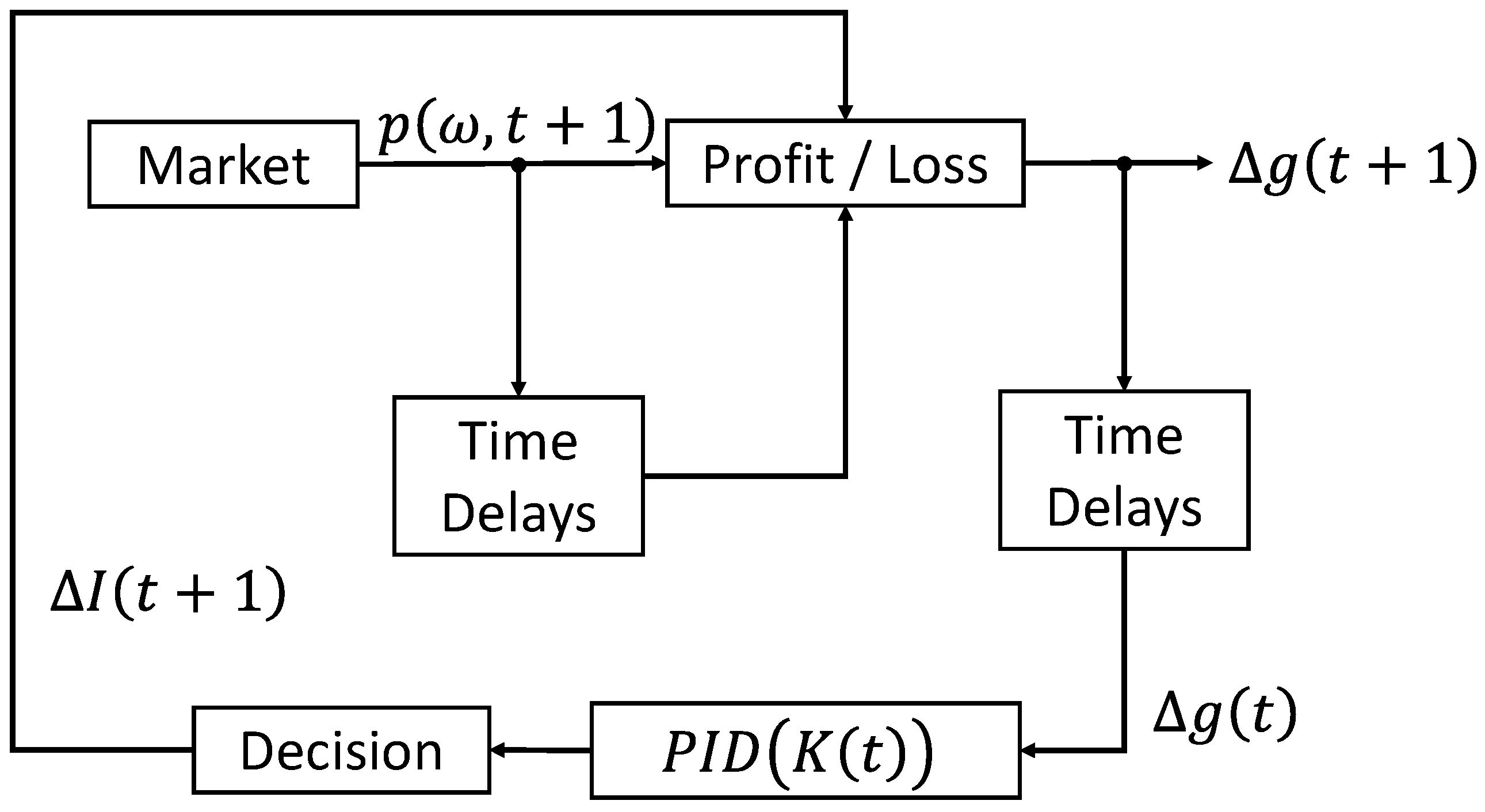
Figure 1. Model-free PID-based trading algorithm.
Jrfm 16 00387 g001
Figure 2. The log-normal like histogram of the ratio θ ( · , t ) for Binance BTC/USDT spot market.
Jrfm 16 00387 g002
Figure 3. The one-day spread dynamics on the Binance BTC/USDT exchange.
Jrfm 16 00387 g003
Figure 4. Binance BTC/USDT one-day price index.
Jrfm 16 00387 g004
Figure 5. Binance BTC/USDT one-day price index.
Jrfm 16 00387 g005
Disclaimer/Publisher’s Note: The statements, opinions and data contained in all publications are solely those of the individual author(s) and contributor(s) and not of MDPI and/or the editor(s). MDPI and/or the editor(s) disclaim responsibility for any injury to people or property resulting from any ideas, methods, instructions or products referred to in the content.