Abstract
Unsteady component interaction represents a crucial topic in turbomachinery design and analysis. Combustor/turbine interaction is one of the most widely studied topics both using experimental and numerical methods due to the risk of failure of high-pressure turbine blades by unexpected deviation of hot flow trajectory and local heat transfer characteristics. Compressor/combustor interaction is also of interest since it has been demonstrated that, under certain conditions, a non-uniform flow field feeds the primary zone of the combustor where the high-pressure compressor blade passing frequency can be clearly individuated. At the integral scale, the relative motion between vanes and blades in compressor and turbine stages governs the aerothermal performance of the gas turbine, especially in the presence of shocks. At the inertial scale, high turbulence levels generated in the combustion chamber govern wall heat transfer in the high-pressure turbine stage, and wakes generated by low-pressure turbine vanes interact with separation bubbles at low-Reynolds conditions by suppressing them. The necessity to correctly analyze these phenomena obliges the scientific community, the industry, and public funding bodies to cooperate and continuously build new test rigs equipped with highly accurate instrumentation to account for real machine effects. In computational fluid dynamics, researchers developed fast and reliable methods to analyze unsteady blade-row interaction in the case of uneven blade count conditions as well as component interaction by using different closures for turbulence in each domain using high-performance computing. This research effort results in countless publications that contribute to unveiling the actual behavior of turbomachinery flow. However, the great number of publications also results in fragmented information that risks being useless in a practical situation. Therefore, it is useful to collect the most relevant outcomes and derive general conclusions that may help the design of next-gen turbomachines. In fact, the necessity to meet the emission limits defined by the Paris agreement in 2015 obliges the turbomachinery community to consider revolutionary cycles in which component interaction plays a crucial role. In the present paper, the authors try to summarize almost 40 years of experimental and numerical research in the component interaction field, aiming at both providing a comprehensive overview and defining the most relevant conclusions obtained in this demanding research field.
1. Introduction
The importance of studying unsteady interaction physics in modern gas turbines has grown during recent years following the improvements of the available design tools. High temperature levels at the combustion chamber exit section combined with the high level of blade load obliged the designers to introduce complex cooling systems and to take into account secondary flow development and wake/blade interaction. The numerical simulation of the flow field inside the turbine stages can provide fundamental information during the design process, but for the described purposes, any steady assumption must be discarded. In fact, vane/blade interaction is mainly a 3D unsteady phenomenon driven by the wake/shock/blade interaction, by secondary flow development and chopping, and by the hot fluid redistribution on the rotating and stationary parts. Moreover, lean-burn combustion technologies generate turbine inlet profiles characterized by high residual swirl, hot spots, and high turbulence levels, thus requiring both high-fidelity tools for numerical simulations and appropriately designed test rigs to account for combustor/turbine interaction. Also, compressor/combustor interaction is a topic of interest due to the possible interaction of combustion instabilities with non-uniform flows from the high-pressure compressor stage. On top of that, limitations in pollutant emissions, in the use of hydrogen blends, and the expected changes in the thermodynamic cycle oblige gas turbine designers to develop new methods for component interaction analysis in unsteady conditions.
Several researchers have already performed experimental and numerical studies to understand unsteady interaction phenomena. Furthermore, a number of numerical methods have been proposed to simulate the unsteady interaction both between different components and at the stage interfaces, the latter made complex by the uneven blade count in compressors and turbines. Thanks to those works, the knowledge of the unsteady phenomena has increased considerably and some general assumptions are accepted as valid in most cases. Nevertheless, every test case features specific characteristics that are connected to the geometrical parameters, the flow field, and the fluid properties. Thus, the study of unsteady interaction in turbomachinery is far from over.
In the present paper, a general introduction about unsteady flows in turbomachinery is presented in Section 2. Unsteady interaction effects are introduced in Section 2.1, then aerothermal interaction is treated (Section 2.2) with special attention paid to secondary flow development (Section 2.3), to the redistribution of non-uniformities (from Section 2.4 to Section 2.7), and to wake/blade (Section 2.8) and shock/blade interactions (Section 2.9). Clocking effects (Section 2.10), loss development (Section 2.11), and aerodynamic instabilities (Section 2.12) are also introduced to the reader. Then, component interaction is discussed in Section 3. Compressor/combustor interaction analysis is reported in Section 3.1, including both test rigs and numerical methods. Then, combustor/turbine interaction is discussed in Section 3.2, which is divided into a part where combustor simulators are reported (Section 3.2.1) and a part where numerical methods are described (Section 3.2.2). Then, numerical methods for blade-row interaction analysis are reported in Section 3.3, with detailed information about the most important ones from Section 3.3.1 to Section 3.3.5. Eventually, conclusions are drawn in Section 4.
2. Unsteady Flows in Gas Turbine Stages
To reach the highest efficiency and specific power values consistently with the characteristics of the materials and of machine reliability is among the most relevant goals of the design process of modern gas turbines. Furthermore, attention has been paid to the emission of unburned hydrocarbons, of nitrates, and of sulfates that are unintentionally produced during the combustion process over the last 20 years due to the necessary reduction in the environmental impact of gas turbines. Then, the effects of component interaction in a gas turbine must be studied along with the behavior of the single components. In fact, both compressor and turbine stage performance depends on the unsteady interaction between the relatively moving rows.
Axial compressors are designed to avoid rotating stall and then a high number of stages with relatively low blade loads are necessary. Concerning the turbines, a lower number of stages is usually present. Also, in the high-pressure stages, the flow is often transonic and blades are highly loaded. This means that in the turbine stages, the flow is strongly 3D and then the unsteady interaction between wakes, secondary flows, and oblique shocks is a complex topic to be studied. Furthermore, the flow coming from the combustion chamber has a high temperature level; the shape of the thermal field at the turbine inlet can introduce unsteady effects if tangential non-uniformities of stagnation temperature are relevant. Finally, both stationary and rotating parts of the stages are subjected to thermo-mechanical fatigue, then a cooling system for the high-pressure turbine stages must be studied to avoid component failure [1,2].
To correctly individuate the most critical components, a deep knowledge of the aerothermal characteristics of the turbine stages is necessary. Even if a purely steady approach may provide a good estimation of the global parameters such as mass flow rate, efficiency, and pressure levels, it cannot give any information about time-resolved variables. Since the thermal field and the global losses are strictly dependent on the unsteady interaction between wakes, shocks, secondary flows, and hot streaks, the steady evaluation must be substituted by the unsteady one.
2.1. Introduction to Unsteady Interaction in Turbomachinery
Unsteady interaction considerably affects the performance parameters of compressors and turbines. Considering a generic stage, the main unsteady sources are usually listed as follows [3]:
- Inlet flow distortions: Boundary conditions affect the performance of the gas turbine (e.g., hot spots and residual swirl from the combustion chamber modify the turbine aerothermal field).
- Potential (inviscid) interaction: It is caused by pressure waves travelling and reflecting across the vane/blade gap.
- Wake unsteadiness: It is mainly represented by vortices developing from vane and blade trailing edges and has an impact on mixing losses and boundary layer development.
- Secondary flows: They are flow structures that deviate from the expected behavior of the flow, and their interaction can produce detrimental effects on turbine performance.
- Oblique shocks from blade trailing edge: In transonic stages, a complex reflecting shock system affects the heat transfer rate due to the generation of separation bubbles.
Furthermore, the following phenomena affecting the compressor may be considered:
- Rotating stall: It is caused by the blockage of some vanes due to the wrong incidence, which causes flow separation.
- Aeroelastic instability: Generally called “flutter”, it is generated by the blade mechanical response to the unsteady disturbance.
Even though these latter phenomena are of paramount importance for the proper design and operation of a compressor, they will only be briefly discussed in the present paper, which is mostly about the turbine module and component interaction analysis.
The unsteady aerodynamics phenomena can be classified according to Table 1.

Table 1.
Overview of main unsteady interaction phenomena.
The characteristic frequencies of the unsteady effects which are associated with the vane/blade interaction are a function of the shaft rotational speed and of the blade count. The periodicity of the wake/blade/shock interaction and of the secondary flow effects is then determined by the working conditions and by the blade number of turbine rows. In these cases, the unsteadiness is defined as “deterministic”. Among the mentioned sources and effects of unsteadiness, a sub-class of self-excited unsteady phenomena consisting of stall, vortex shedding, and flutter can be individuated. Their frequency is not completely ascribable to the geometrical properties of the turbine, so this kind of unsteadiness is usually defined as “stochastic” [4].
As is shown in Section 2.2, Section 2.3, Section 2.4, Section 2.5, Section 2.6, Section 2.7, Section 2.8, Section 2.9, Section 2.10, Section 2.11 and Section 2.12, all those phenomena interact with each other and a clear distinction of the separated effects on the aerothermal field is a complex exercise. However, comments can be made by considering their main features.
2.2. Potential Interaction in Turbine Stages
Unsteady disturbances travel in terms of flow characteristics. Considering a turbine stage where v is the local flow velocity, there are four main disturbances travelling across the blade row gap:
- Entropy and velocity fluctuations are convected downstream of the vane row at the local flow velocity v.
- Pressure fluctuations travel as acoustic waves at and velocities (a being the local speed of sound), then the direction changes depending on flow regime, which can be either subsonic (, where is the Mach number) or supersonic ().
- Wakes generated by vanes represent a source of unsteadiness for the blade row. Since the pressure gradient across a wake is negligible, wake disturbance travels at a velocity that is lower than the one associated with the main flow. This is the driving mechanism for the “negative jet” effect, which is responsible for a fundamental interaction phenomenon occurring in aero-engines at cruise conditions in low-pressure turbine stages (see Section 2.8).
- Steady pressure field associated with the blade load is a source of unsteadiness for the adjacent rows. Since this mechanism is purely inviscid, this kind of interaction is referred to as “potential”.
In turbines, the blade loading and the flow speed are higher in the rear part of the row, then the potential interaction with the downstream row is stronger than the one occurring with the upstream row. An equation has been proposed by Parker [5] to evaluate the rate of decay of potential interactions upstream and downstream of a cascade. Considering a low-speed turbine, the relation is reported in Equation (1).
The decay rate is a function of both the axial gap x divided by the blade pitch S and of the Mach number calculated using the rotational velocity of the blade row . For low-speed turbines, an axial gap of of the blade pitch is already sufficient to strongly smooth the potential interaction, while after one pitch, the flow can be considered steady.
For high-speed turbines, Greitzer [6] proposed a function of the intra-row gap and of the axial and rotational Mach number, thus associating the potential interaction intensity to the dimensionless axial velocity non-uniformity. Assuming a value of for the ratio between the axial velocity and the rotational velocity in transonic turbines, for low values of the rotational velocity, Greitzer [6] obtained the same results obtained by Parker [5]. On the contrary, when increasing the rotational velocity (thus moving towards transitional flows), the rate of decay decreased strongly, and for high rotational velocity values, there was no visible decay.
It can be observed that even if the potential interaction is an important source of unsteadiness travelling up- and downstream of the stage, its relevance in transonic and supersonic turbine stages is weakened by the presence of complex shock reflection systems that modify the intra-row pressure and velocity fields (see Section 2.9). Furthermore, secondary flows (Section 2.3), hot spots (Section 2.5), and residual swirl (Section 2.6) concur to increase the overall complexity of calculating the contributions to unsteady losses in turbine stages.
2.3. Secondary Flows in Turbomachinery
All the flow structures that deviate from the expected behavior in a channel can be defined as “secondary flows”. Among the studies that aim at defining these flows, it is worth citing Sieverding [7] and Langston [8].
The most relevant secondary flows occurring in turbine stages are the “passage vortex”, the “horseshoe vortex”, and the “tip leakage vortex”. The passage vortex is generated by the boundary layer behavior in a curved vane. Considering an intrinsic coordinate system, the pressure gradient in the direction normal to the stream-wise direction is balanced by the centrifugal force calculated using the stream-wise velocity and the local curvature of the streamline R. Since the flow velocity in the boundary layer is lower than in the inviscid region and the pressure gradient in the bi-normal direction b (locally defined as ) is nil, the local curvature radius R diminishes (thus maintaining unaltered the centrifugal force) and two counter-rotating vortices are generated close to the vane end-walls. That behavior can be explained by considering boundary layer equations in the intrinsic system reported in Equation (2).
The fluid near the end-walls moves toward the blade suction side while the fluid near the mid-span is transported towards the pressure side. A visualization of the two branches of the passage vortex is reported in Figure 1, where and are visible for a transonic high-pressure blade along with the time-averaged entropy variation () map calculated at the blade exit section. Figure 1 is obtained using the numerical results shown by Salvadori et al. [9] for a uniform turbine inlet condition, where a detailed description of the numerical approach is also reported. The time-averaged values in the map are scaled using a reference condition that results in kJ/kg at the lowest entropy value on that section, so that the zones where the losses are relevant can be easily individuated. Therefore, the map is only meant to track the position of the secondary flows for visualization purposes. Figure 1 also shows that the streamlines positioned close to the mid-span are almost unaffected by the presence of secondary flows. In fact, the impact of the passage vortex on the flow field is reduced when increasing the aspect ratio of the vane since a limited portion of the domain is interested by boundary layer effects.
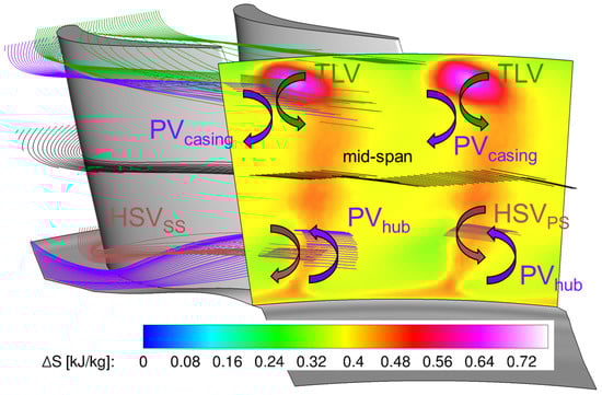
Figure 1.
Secondary flow visualization in a high-pressure turbine blade.
At the blade leading edge in the boundary layer zone, the flow is divided by the stagnation line into two counter-rotating vortices that move inside of two adjacent vanes. With reference to Figure 2, which is also obtained using numerical data from Salvadori et al. [9], both the branches of the horseshoe vortex obtained for a transonic high-pressure blade move towards the blade suction sides. Figure 2 also shows the non-dimensional map of static pressure p (normalized with respect to the stage inlet mean total pressure value) on the lower end-wall, thus evidencing the pressure gradient that occurs in that portion of passage. The “pressure side leg” of the horseshoe vortex moves towards the suction side because of the pressure gradient between pressure and suction side and interacts with the lower branch of the passage vortex that has the same direction of rotation, as visible in Figure 1. On the contrary, the “suction side leg” of the horseshoe vortex is counter-rotating with respect to the passage vortex and remains close to the blade surface. Even though is clearly visible in Figure 1, some authors suggest that its development is mainly counteracted by the presence of the and that it remains close to the end-wall, thus contributing to the formation of the so-called “corner vortex”.
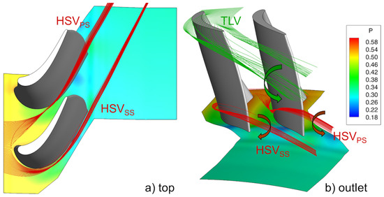
Figure 2.
Visualization of the horseshoe vortex and of the tip leakage vortex in a high-pressure turbine blade along with the non-dimensional static pressure map on the lower end-wall.
In unshrouded blades, a percentage of the flow migrates from the pressure to the suction side of the blade through the clearance between the blade tip and the casing. That phenomenon can be identified in Figure 2 by looking at the streamlines designed close to the blade tip. With reference to Figure 1, the tip leakage vortex is counter-rotating with respect to the passage vortex and has comparable (or higher) intensity, thus moving the branch towards mid-span. The tip leakage vortex represents one of the most important loss mechanisms in transonic turbine stages, as demonstrated by the increased entropy values associated with the in Figure 1 at the blade exit section.
Among the other secondary flows, the trailing edge vortex (which develops within the base region), the scraping vortex (which develops close to the casing in unshrouded blades), and the corner vortex (which is sometimes associated with the “suction side leg” of the horseshoe vortex) can be mentioned. A complete description of these flows can be found in Lakshminarayana [1], Sieverding [7], Langston [8,10], and Délery [11]. The magnitude of the secondary flows is sometimes measured in terms of secondary vorticity. A generalized expression for the secondary vorticity have been proposed by Lakshminarayana and Horlock [12], where the variation of vorticity was correlated with its redistribution, diffusion, and production considering a fluid with a given viscosity and the density, velocity, and pressure gradients. This equation is currently a reference for anyone who studies secondary flow development in turbines.
The presence of secondary flows is associated with the reduction in stagnation pressure and an increase in overall losses [13]. Moreover, the vortices developed in the upstream row are partially mixed out and are chopped by the downstream row, thus representing incoming secondary vorticity for low-pressure stages. Also, some secondary flows interact with other unsteady phenomena like the “segregation effect” [14,15] (which will be extensively described in Section 2.5). Therefore, their correct evaluation is fundamental for the calculation of both flow incidence on the blade and the overall turbine performance [16,17]. To weaken both the passage and the horseshoe vortices, some obstacles (e.g., fences and grooves) can be used. Moreover, the control of the passage vortex can be obtained by using end-wall contouring or blade leaning. A detailed description of these methodologies is out of the scope of the present paper and more information can be found in the cited papers.
2.4. Stagnation Pressure Non-Uniformity at the Combustor Exit
Due to the complexity of the flow field inside of a combustion chamber, it might seem reasonable to suppose the presence of stagnation pressure non-uniformity on its exit section. Some works reported a map of stagnation pressure downstream combustion chambers or hot streak generators. Two examples were shown in Qureshi et al. [18], where the experimentally measured stagnation pressure distribution downstream of a hot streak generator was shown, and Shahpar and Caloni [19], where the stagnation pressure obtained numerically downstream of a lean-burn combustor was shown. Despite a qualitative difference in the maps, both the distributions were characterized by a narrow range of variation, with the maximum non-uniformity lower than .
In the case of Qureshi et al. [18], it was not possible to observe organized structures due to the low resolution of the experiments. On the contrary, the case in Shahpar and Caloni [19] allowed some aspects to be distinguished. The zone with the lower stagnation pressure was located in the central part of the channel height and overlapped with the swirl core. Moreover, it was possible to hypothesize that the high stagnation pressure bands positioned near the end-walls were due to the coolant flow injected upstream to protect the combustor walls. A behavior similar to the one shown in Shahpar and Caloni [19] was observed by Hall et al. [20] on a hot streak generator, both in qualitative and quantitative terms. However, a non-negligible impact of inlet stagnation pressure profile on the development of secondary flows and in the redistribution of cold flow in high-pressure vanes was found by Barringer et al. [21,22], as discussed in Section 2.5.
It is possible to conclude that stagnation pressure non-uniformities on the combustor/turbine interface do not constitute a primary aspect of the interaction between combustors and high-pressure turbine stages, at least for most of the investigated cases.
2.5. Hot Spot Migration in the High-Pressure Turbine Stage
The continuous increase in turbine inlet temperature produced a high thermal load that a turbine can withstand thanks to the increased efficiency of cooling systems and of the manufacturing technology. Considering the thermal resistance, a crucial issue is represented by both the temperature and the heat transfer coefficient maps on the blade surfaces. Furthermore, the interest in secondary component design has acquired more attention, moving the investigations towards the heat transfer evaluation at the end-walls.
The shape of the inlet stagnation temperature field generated by modern combustion chambers needs to be accounted for. In fact, important changes introduced by both Dry Low (DLN) and lean-burn technologies in the burner design obliged the researchers to evaluate the effects of radial and circumferential hot spots of temperature on the performance of the high-pressure turbine stages. An explanation of how the hot spot is generated inside of a lean-burn combustor is reported in Figure 3 for a case study [23] simulated by Insinna et al. [24].
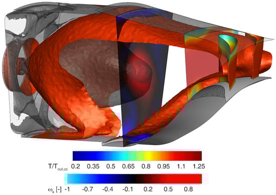
Figure 3.
Hot spot generation in a lean-burn combustor coupled with a high-pressure turbine vane.
In Figure 3, a grey iso-surface where the flow velocity is nil is reported to make evident the flow recirculation zone occurring in the primary zone. The colored iso-surface represents the region where , which is approximately where K. This allows for individuating two regions close to the liner where flow temperature is greatly reduced by the presence of cooling slots, thus generating the typical radial temperature profile. It also has an impact on the generation of the 2D temperature profile occurring at the turbine inlet section, which is also visible in Figure 4 along with both the velocity map and the Radial Temperature Distortion Factor . The latter is defined as in Equation (3) using the stagnation temperature , where stands for the local time-averaged value, the term stands for the mean value of the time-averaged values, and the denominator is calculated as the mean difference across the combustion chamber .
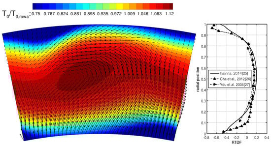
Figure 4.
Aerothermal field on the combustor/turbine interface (adapted from [25,26,27]).
As can be observed, the hot spot is positioned approximately in the center of the section and is correlated to the residual swirl coming from the primary zone, as demonstrated by the 2D map of axial vorticity reported in Figure 3 on a plane positioned at the entrance of the transition piece. Concerning the values reported in Figure 4, the distribution obtained by Insinna [25] is compared with the ones obtained by Cha et al. [26] and by You et al. [27], thus demonstrating its representativeness for lean-burn combustors. A detailed analysis of the lateral migration of the hot spot can be found in the work by Insinna et al. [24].
Inside the vanes, these non-uniform temperature distributions become “hot streaks” that tend to move towards the blade pressure side and then migrate both through the tip clearance and towards the lower end-wall (or “hub”). The mechanism of redistribution of a hot spot is a complex unsteady phenomenon that is influenced by many parameters. One of the first experimental studies about hot streak migration was conducted by Butler et al. [28], who created a hot streak injecting hot fluid scattered by CO2 through a pipe aligned with the vane and positioned at mid-span. Following CO2 migration, they showed that in an axial machine, the hot fluid tends to accumulate on the pressure side of the high-pressure turbine blades. This result was explained by considering that according to Munk and Prim [29], for a steady isentropic flow without body forces, given a prescribed geometry and with a defined stagnation pressure inlet field, the streamlines, the Mach number, and the static pressure fields at the outlet were not influenced by the stagnation temperature inlet field. That means that at the vane exit section, the hot fluid had a higher velocity than the surrounding one, triggering the “segregation effect” mechanism that was evidenced for the first time by Kerrebrock and Mikolajczak [14] when treating the wake transport inside compressors. However, it could be used to explain the preferential migration of hot fluid towards the pressure side of the high-pressure turbine blades.
The velocity triangles at the vane exit section are characterized by an absolute angle that guarantees the optimal incidence on the blades in the relative frame of reference. The composition of the velocity triangle is governed by a simple relation between vectors, namely . In Figure 5, three different velocity profiles that may occur at the vane exit section are reported, where stands for the nominal (or design) condition, for the hot flow, and for the wake flow. Recalling the substitution principle, the hot flow has the same absolute stagnation pressure of the surrounding fluid and a higher absolute velocity intensity . The opposite happens to the wake flow, which is characterized by a reduced absolute velocity intensity . Therefore, looking at the velocity triangles, the blade stagnation point moves towards the pressure side for the hot fluid and towards the suction side for the wake flow. Moreover, when composing the relative velocities and with , two slip velocities appear for the hot () and the cold () flow. These two slip velocities are called “positive jet” and “negative jet” and are responsible for the relative movement of the hot flow towards the pressure side and of the wake flow towards the suction side, respectively.
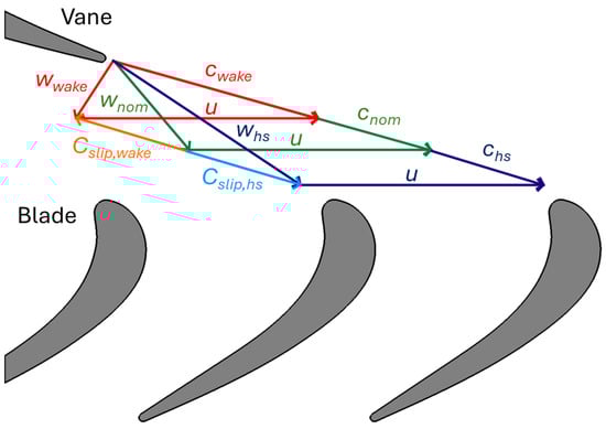
Figure 5.
Definition of slip velocity components in turbine stages.
These two effects are visible in Figure 6, where the fluctuating flow field in the relative frame of reference is calculated at mid-span as and is overlapped with the time-resolved temperature map at two different instants of the numerical simulation performed by Salvadori et al. [9] in the case of a hot spot aligned with the vane passage. As can be observed, at time , the relative motion of the hot flow brings the fluid towards the blade pressure side, thus increasing its heat load. After half period, at , the wake flow enters the blade passage and moves preferentially towards the suction side. It can also be observed that for the investigated case, two counter-rotating “segregation vortices” (labelled as A and B in Figure 6) are generated by the relative motion of the flow and are stretched while travelling across the passage, thus contributing to the generation of aerodynamic losses. From a thermal point of view, the preferential migration of the hot fluid towards the pressure side interacts with the passage vortex and leads to both the formation of a fluctuating hot region [9] and the increase in the blade load [30] due to the positive incidence at the leading edge. These two effects cannot be predicted by considering either uniform inlet conditions or a steady flow assumption or a 2D problem. In fact, Butler et al. [28] performed a 2D Euler steady simulation at the mid-span of a test rig and observed that temperature values were lower than experimental ones. This discrepancy was mainly caused by the “mixing plane” technique that eliminates the segregation effect. Later, an unsteady 2D simulation made by Rai and Dring [31] on the same test rig showed that temperature levels were higher than the results obtained by Butler et al. [28], but were still lower than the experiments. The reason for that under-prediction was the missing interaction of the positive jet with secondary flows. Finally, Dorney et al. [15] carried out an unsteady 3D simulation demonstrating the mechanism that ruled the interaction between the segregation effect and the passage vortex. They showed that the secondary redistribution brought the hot fluid from suction to pressure side across the vane, thus enhancing the segregation effect and spreading the hot fluid over the pressure surface of the blade, up to the tip clearance.
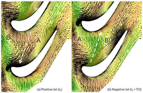
Figure 6.
Segregation effect generated by positive and negative jet.
Temperature non-uniformities also modify the strength of secondary flows. Considering the expression of vorticity by Lakshminarayana and Horlock [12] for a compressible, axisymmetric flow with negligible axial gradients compared to radial ones, the experimental analysis by Butler et al. [28] showed that the vorticity level was higher in the presence of hot streaks than without. All the experimental and numerical analysis that followed that study [28] confirmed that the segregation effect was the dominant mechanism of redistribution of hot fluid in the rotational frame of reference.
For all those reasons, the migration of the hot spot originating from a combustion chamber needs to be accounted for using unsteady 3D approaches, at least during the final steps of a design process to guarantee the proper functioning of cooling systems and appropriate safety margins. Detailed analyses of hot spot redistribution in a high-pressure turbine stage are available in the experimental and numerical studies performed by Salvadori et al. [9], Povey et al. [32], Adami et al. [33], and Simone et al. [30]. Those studies were conducted on the research high-pressure turbine stage MT1 designed by Rolls-Royce and tested at the Isentropic Light Piston Facility (ILPF) [34,35].
Povey et al. [32] studied the effect of two differently clocked hot spots on vane and end-wall heat transfer. The stagnation temperature non-uniformities used for the experimental campaign were characterized by a value up to for the vane-aligned case, and were referred to as Overall Temperature Distortion Factor (OTDF) [35,36,37]. Considering the corresponding RTDF defined in Equation (3), the value was reduced to for both the alignments. The OTDFs were generated through an Inlet Temperature Distortion (ITD) generator by blowing cool air through struts positioned upstream of the high-pressure turbine vanes [38]. The high-pressure turbine stage was composed of 32 vanes and 60 blades and the number of hot spots was equal to the number of vanes. Povey et al. [32] showed that with respect to results obtained considering a uniformly distributed inlet profile, the heat transfer rate on vane suction side at mid-span was substantially increased by aligning the hot spot to the leading edge, while it was slightly reduced if the hot spot was aligned to the passage. On the contrary, heat transfer on the pressure side at mid-span was insensitive to changes in the position of the ITD. Concerning the end-walls, heat transfer rate greatly decreases with respect to the uniform case due to the reduced temperature level close to the end-walls associated with the OTDF map. The latter result was also insensitive to the ITD clocking, and suggested that the presence of hot spots may be beneficial for high-pressure turbine end-walls in terms of heat load.
Adami et al. [33] performed unsteady simulations of the MT1 stage with and without a temperature distortion. Concerning the latter, only the passage-aligned profile reported in [32] was considered and then rotated to study clocking effect. Numerical results were compared to the available experimental data, thus allowing for a detailed validation of the numerical method and a comprehensive analysis of hot spot redistribution both in the blade passage and through the tip leakage. The quasi-homothetic scaling of the blade adopted by Adami et al. [33] allowed for obtaining a 32:64 blade count that made the unsteady simulation affordable considering only one vane and two blades. A “sliding plane” approach was used with a numerical sampling frequency of 1.27 MHz, which was higher than the experimental one. Results obtained by Adami et al. [33] compared well with the experimental distribution of the isentropic Mach number at three vane heights. On the contrary, numerical results on the blade predicted a lower blade load than expected, which was a significant flaw of the so-called “domain scaling” approach, at least in this case where a Scaling Factor (SF) of ≈7% was necessary (see Section 3.3.1 for more information on this unsteady method). That conclusion was investigated further in the paper by Salvadori et al. [9], where results obtained using the actual blade count of 32:60 using the ELSA solver developed at ONERA (FR) were presented thanks to the usage of “phase lagged” boundary conditions. Results obtained by [33] confirmed that vane aerodynamics were not affected by the presence of the OTDF, coherently with the “substitution principle” by Munk and Prim [29]. On the contrary, heat transfer rate on vane suction side was increased when the hot spot was aligned to the leading edge, as also concluded in [32], while no relevant variation was associated with the alignment to the vane passage.
Concerning the blade passage, Adami et al. [33] tracked the hot flow redistribution by means of entropy contours. They demonstrated that if the hot spot is aligned to the vane passage, the redistribution mechanism described by Kerrebrock and Mikolajczak [14] was more pronounced since the hot spot travelled across the vane almost unchanged and the slip velocity component in the relative frame was higher than for the vane-aligned case. In fact, in the latter case, the positive jet effect was weakened by the interaction with the wake. Unfortunately, the relatively low value of ≈1.07 associated with the investigated OTDF did not allow for a well-defined visualization of Nusselt number increase on blade pressure side.
Salvadori et al. [9] performed an experimental and numerical campaign considering the new ITD generator by Qureshi et al. [18] that allowed for reaching a of ≈1.2 and a temperature profile more representative of a gas turbine combustor. Results obtained both with the in-house solver HybFlow originally developed at the University of Florence (IT) and with the ELSA solver developed at ONERA (FR) since 1997 were shown. Experimental results obtained using the ILPF at QinetiQ (UK) supported the validation of the numerical approaches and the data analysis. All the numerical results confirmed that vane aerodynamics were not affected either by the shape or the clocking of the hot spot. On the contrary, time-averaged isentropic Mach number distribution at blade mid-span showed that a non-negligible value was responsible for an increased blade load due to the positive incidence associated with the positive jet effect. That outcome is also demonstrated by the unsteady blade load, which was increased by a factor of ≈6.5% in the presence of an enhanced OTDF. Results obtained by using “phase lagged” boundary conditions [39] implemented in ELSA [40] were in line with the experimental data and were able to correctly capture inter-stage pressure level, which was, on the contrary, over-estimated when using the “domain scaling” approach. Concerning heat transfer, all the calculations agreed that the Nusselt number values on blade pressure side at mid-span in the presence of a hot spot were higher than in the case of uniform inlet profile due to the positive jet effect and its interaction with the passage vortex. Nusselt number distribution at other heights greatly depended on the RTDF associated with each OTDF profile. However, numerical simulations captured the redistribution mechanism associated with the radial movement of the hot flow generated by the passage vortex, which ultimately brought the hot flow through the tip clearance and increased the Nusselt number on blade suction side close to the upper end-wall. Nevertheless, neither hot spot intensity nor clocking had a relevant impact on the casing heat transfer, which was dominated by the compression mechanism of the leakage flow through the tip clearance, as shown by numerical simulations. However, the latter conclusion was partially in contrast with the experimental data published by [36] on the blade tip, who showed a remarkable increase in Nusselt number at half chord in the presence of a weak hot spot aligned to the vane leading edge. It must be underscored that an experimental and numerical campaign performed by Thorpe et al. [41] on a transonic turbine stage without inlet non-uniformities already demonstrated that large spatial and temporal variations in the instantaneous heat flux on the over-tip region are present. The analysis of the time-resolved numerical results allowed for associating more than half of the local heat load to the leakage flow through the tip clearance. Thorpe et al. [41] calculated that at the mid-chord section, the leakage flow causes a heat load increase by . Furthermore, in the tip gap, the stagnation temperature increased of about of the stage stagnation temperature variation. This change was caused by the isentropic work addition to the flow within the gap, thus confirming the outcome obtained by Salvadori et al. [9]. It may be concluded that the heat load in the over-tip region was a function of both inlet distortions and secondary flow development, the latter being the dominant mechanism.
Qureshi et al. [18] studied the impact of the same enhanced OTDF profile used in [9] to determine to what extent it modified the temperature level on the vane surface and on the end-walls. Again, vane aerodynamics were not affected by the presence of the hot spot. On the contrary, significant span-wise variations in heat transfer associated with the presence of the enhanced OTDF were found, the variation in local temperature values being the driving mechanism. On the end-walls, heat transfer maps were driven by the development of secondary flows, and the heat load was reduced thanks to the radial temperature profile imposed at the entrance of the vane.
Simone et al. [30] analyzed in detail the aerothermal effect of the enhanced OTDF [18] aligned with the vane leading edge by comparing isentropic Mach number and Nusselt distributions on both solid walls and at the stage exit section with data obtained by imposing a uniform inlet profile. Both experimental and numerical data were used, thus allowing for validating the numerical approach for both the investigated cases. The unsteady approach was the same as described in [9] for the in-house HybFlow solver, which effectively reproduced all the experimental data except for the blade load, due to the limitations of the “domain scaling” approach. A negligible impact of the OTDF on vane load was confirmed as well as a higher acceleration of the flow by a factor of on blade suction side close to the leading edge, caused by the positive jet effect. At vane mid-span, Nusselt number increased by on suction side and by on pressure side, thus suggesting that the hot flow moved towards the most accelerating region of the vane. Moreover, Simone et al. [30] quantified that the increase in Nusselt number was ≈60% on the pressure side of the blade, close to the trailing edge, thus confirming the thermal impact of the positive jet effect combined with the passage vortex. Based on these results, Montomoli et al. [4] evaluated that an increase in blade metal temperature of ≈40 K may be responsible for a residual life decrease by . Moreover, a residual unsteady hot spot characterized by a peak temperature by with respect to the uniform case was individuated at stage exit Simone et al. [30], which may lead to harmful conditions for the second stage vane.
Several experimental and numerical investigations with boundary conditions other than the ones from [35,36,37] were performed. Roback and Dring [42,43] studied experimentally the differences between blade temperature fields obtained with a hot streak, a cold streak (a cold spot aligned with the vane), and phantom cooling. Furthermore, they tried to move the hot spot position both tangentially and radially. They showed that by aligning the hot streak to the vane leading edge, the thermal load on the blade was reduced. In fact, the hot fluid moves on vane suction side and interacts with vane wake. This interaction weakened the strength of the segregation effect and generated a more uniform distribution of temperature field. This kind of solution may help control the blade temperature but requires dedicated study of vane cooling systems.
Dorney and Gundy-Burlet [44], Gundy-Burlet and Dorney [45] studied hot streaks, clocking effects, and heat transfer with an unsteady 3D isothermal simulation. The latter study showed that neither hot streaks nor blade metal temperature influence time-averaged behavior of isentropic Mach number on the blade surface. Shang and Epstein [46] proposed a numerical study of the span-wise migration of hot fluid on the blade pressure side. Using an unsteady 3D Euler solver, they showed that the hot fluid moves towards the lower end-wall. Furthermore, they demonstrated that the potential interaction between hot fluid and the blades was not the main feature in hot streak redistribution. In fact, clocking effects generated a non-uniform time-averaged temperature distribution in the vane/blade interface.
He et al. [47] tested two different relative alignments between vanes and hot spots with two different numbers, namely the hot spot alignment with the leading edge and the vane passage. Two different hot spot counts were used, with hot spot-to-vane ratios of 1:4 and 1:1. The shapes of the inlet stagnation temperature distortions were sinusoidal in both radial and tangential directions and were characterized by ratio. The test rig used for the analysis was the one described in Povey and Qureshi [37]. Results showed that, for the 1:1 case, the blade thermal load was strongly dependent on the hot streak/vane clocking, while the aerodynamic forcing was almost independent of it. On the contrary, for the 1:4 case, clocking had a limited effect in determining the adiabatic blade temperature, whereas the unsteady forcing on the blades was at least five times higher than for the 1:1 case. Although such results had been obtained with theoretical stagnation temperature inlet distributions without considering any other type of flow distortion coming from the combustor (e.g., residual swirl), they gave important information concerning the necessity of considering combustor/turbine interaction during the aerothermal design of gas turbines.
The interaction between the shocks and the hot streaks was studied by Saxer and Felici [48]. They concluded that the local increase in heat transfer was mainly caused by the position of the oblique shock impingement on the blade and by the clocking effects between the hot streak, the blade number, and the relative position. Some experimental and numerical studies concerning the hot spot shape [49], the tip clearance effects Dorney and Sondak [50], and the multistage aspects [51,52] were performed, too.
Barringer et al. [21,22,53,54] developed an inlet profiled generator to perform high-pressure turbine tests. The device demonstrated that it could reproduce a variety of turbine inlet profiles at engine relevant conditions with realistic turbulence levels [53]. Results obtained by testing several temperature and pressure radial profiles suggested that it is theoretically possible to individuate an ideal pressure profile that reduces the secondary flows and the heat load to the turbine [54]. The highest benefit in terms of heat transfer was associated with the temperature profile with the largest radial gradient. The authors also described the thermal migration process in the span-wise direction associated with the vane inlet pressure profile type, also underlining that attention must be paid to the driving temperature used to predict Nusselt number distribution on vane surfaces and end-walls [54]. Concerning the latter, Barringer et al. [21] demonstrated that Nusselt number distribution was highly dependent on the inlet pressure profile, with higher Nusselt numbers associated with inlet profiles coherent with a standard turbulent boundary layer with respect to a case with higher stagnation pressure near the end-wall. Moreover, the validity of the assumption of a constant freestream temperature as a heat transfer driving mechanism was discussed, concluding that it may result in the wrong prediction of local heat transfer coefficients [21]. The migration of combustor exit profiles in high-pressure vanes was also analyzed by considering several different radial profiles of pressure and temperature in a fully annular ring (Barringer et al. [22]). As the stagnation pressure near the end-wall increased, stagnation pressure losses through the vane increased due to the development of stronger secondary flows. The latter also governed temperature distributions close to the inner and outer diameter end-walls, the relatively cold flow being redistributed within the passage depending on the inlet stagnation pressure radial distribution. Moreover, an increase in inlet stagnation pressure near the end-walls resulted in a reduced turning of the flow within the passage, which may affect the performance of the downstream blade (Barringer et al. [22]).
Mathison et al. [55,56,57] performed several experimental studies about aerodynamics and heat transfer of a cooled one-and-a-half high-pressure turbine stage with inlet temperature distortions. The authors described the main characteristics of both the cooled turbine stage and the combustor emulator, also including the main characteristics of the experimental setup and comparing the outcome in terms of temperature profiles with the existing literature [55]. They found that a radial temperature distribution at the stage inlet was responsible for the migration of the peak of high metal temperature from to span in the blade channel, caused also by the presence of tip leakage [56]. They also found that the impact of the segregation effect increased when increasing the temperature distortion. Moreover, an increased coolant flow rate from the vane increased the impact of the segregation effect since the cold flow moved towards blade suction side, coherently with what was described by Roback and Dring [42,43]. Time-accurate measurements demonstrated that a purely radial inlet temperature distribution generated similar temperature patterns on all the vane passages, while hot spot alignment had a severe impact on blade heat transfer [56]. When the hot spot was aligned with the cooled vane leading edge, the mixing between hot and cold flow virtually eliminated temperature peaks associated with the inlet non-uniformity (at least in the conditions reported in [55]). On the contrary, if the hot spot was aligned with the vane passage, the mixing was greatly limited and the segregation effect was clearly individuated on blade surfaces [56].
Among the phenomena usually associated with the entrainment of a hot spot in compressible flow in a channel, the unsteady convection of entropy waves recently obtained a high level of interest from the scientific community, both through experimental and numerical studies. This is caused by the fact that a certain level of losses is associated with the “entropy noise” phenomenon, thus justifying the presence of several studies by researchers in the turbomachinery field thanks to its similarity to hot spot redistribution in high-pressure turbine vanes. However, entropy noise is not strictly associated with the aerodynamic and heat transfer problems discussed in the present paper and is not going to be detailed here. For those who are interested in studying this challenging topic, the works by Gaetani and Persico [58], Gaetani et al. [59], Pinelli et al. [60], Notaristefano and Gaetani [61,62,63], and Pinelli et al. [64] are suggested.
2.6. Residual Swirl on Turbine Inlet Section
Modern low-emission combustion chambers adopt swirling flows to provide an adequate flame stabilization. A high swirl number is imposed to the flow by means of appropriate systems located in the burners. The definition of swirl number , typically used to characterize swirling flows, is given in Equation (4), where is the axial flux of tangential momentum, is the outer radius of the duct from which the swirl is originated, and is the axial flux of the axial momentum.
Swirl numbers higher than are often adopted in modern combustors. The intensity of the tangential velocity component makes the swirl persist downstream, up to the high-pressure turbine vanes (see Figure 4). This is particularly important for lean-burn combustors, where two aspects contribute to maintaining swirl up to the combustor exit section. The first one is the use high swirl numbers and the second one is connected to the reduction in dilution jets, which would contribute to dissipating swirl. An example of this configuration is reported in Figure 3.
The work by Shahpar and Caloni [19] reported the yaw and pitch angle distributions obtained numerically on the outlet section of a lean-burn aero-engine combustor. Shahpar and Caloni [19] observed that an organized flow distortion was present, indicating that combustor swirl was conserved up to the exit section. For this particular case, the maximum and minimum yaw angles were, respectively, near the hub and near the casing, while the pitch angle ranged from near the casing to near the hub. Some works had also investigated the effects of swirl on the aerothermal behavior of the high-pressure turbine. Qureshi et al. [65,66] used an annular device consisting of 16 swirl generators, each of them being composed by six stationary flat-plate vanes inclined by an angle of with respect to the axial direction. The generated swirl was experimentally measured in the Oxford Turbine Research Facility (OTRF) and was reported in the form of vector plot and yaw angle distributions at and of the radial position. The swirl intensity in proximity to the end-walls was also quantified, and is characterized by maximum and minimum peaks of yaw angle, respectively, equal to about and .
Qureshi et al. [65,66] applied such a swirl profile to the inlet section of the MT1 high-pressure turbine stage, investigating experimentally and numerically its impact on vane aerodynamics. In this case, the ratio between vanes and swirlers was 1:2 (16 swirlers and 32 vanes), while the blade count was 60 blades. Results showed that the vane aerodynamics were considerably altered by swirl, resulting in relevant changes in loading distributions at and span caused by the movement of the stagnation points towards the pressure side and the suction side, respectively [65]. Therefore, the development of secondary flows was considerably altered as well as the pattern of core losses at the vane exit section. Nusselt number distributions on vane and end-walls were also modified due to streamline convergence and divergence caused by the presence of the swirl. The swirl alignment analysis also showed that the streamlines were strongly redistributed on the pressure side of the vane that was aligned to the swirler, thus suggesting that the design of the cooling system for high-pressure vanes should be verified in the presence of realistic inlet conditions [65]. The presence of a strong residual swirl also affected flow incidence on the blade, with angle variations up to from mid-span to tip and up to near the hub with respect to the uniform inlet case [66]. These incidence variations modified the structure of the flow pattern within the blade passage itself, also impacting on the heat transfer along the casing, where the experiments with inlet swirl showed an increment of in the Nusselt number with respect to the uniform case. In terms of Nusselt number along the blade surface, an increase between and was observed on the suction side. It was attributed to the enhanced turbulence intensity with inlet swirl. On the pressure side, an increment in the Nusselt number of about near the hub and up to near the tip was observed. Such a significant increase in the upper part of the blade was mainly due to increased tip leakage flow intensity [66].
Schmid and Schiffer [67] studied a linear cascade of nozzle guide vanes by means of numerical simulations, including inlet swirl vortices in a 1:1 ratio with respect to the vane counts. They considered three different swirl numbers, equal to , , and , as well as three different swirl orientations (clockwise, counter-clockwise, and counter-rotating). Results showed that an increase in the swirl intensity was accompanied by a strong increase in the stagnation pressure loss coefficient, which ranged from of the value obtained with axial flow for to for . Moreover, remarkable effects of the swirl orientation were also observed. Schmid and Schiffer [67] concluded that when the swirling flow near the hub was almost orthogonal to the vane orientation (clockwise case), the saddle point of the streamlines impacting on the vane surface moved towards the pressure side. The opposite happened for the counter-clockwise case, for which the saddle point moved towards the suction side. A different situation occurred when alternate swirl directions were used for the adjacent vanes (counter-rotating case). In this case, the flow features were different from the two aforementioned cases and the two vanes worked differently from one another. The complex flow feature created in the clockwise and the counter rotating cases generated local increases in the heat transfer coefficient, which could be potentially harmful for the metal component from the thermal point of view.
Khanal et al. [68] investigated numerically the hot streak transport in the MT1 high-pressure turbine stage with the contemporary presence of an inlet swirl and a hot spot centered on the swirl core. They considered two different relative alignments between swirl and vanes: a swirl aligned to the vane leading edge and a swirl aligned with the passage. Moreover, for each of these cases, they considered positive and negative swirl directions. A case with the hot spot only, without swirl, was also taken into account for each of the alignments. The swirl is responsible for determining the radial migration of the hot streak inside the vane passages, which affects the temperature distortion on the inlet section of the downstream blade. In fact, for all the analyzed cases, the shape of the hot streak was different from the case without swirl. In particular, considering the vane-aligned cases, when a positive swirl was used, the highest temperatures were found near the casing on the pressure side and near the hub on the suction side. The opposite happened for negative swirl. When the passage-aligned cases were considered, the positive swirl redistributed the hot streak in the pitch-wise direction inside of the passage in the medium/high part of the span, while the hot fluid was confined in the center of the passage in the lower part of the channel. A similar behavior was found for the negative swirl case, even if the region near the casing was less thermally loaded and the hot streak less extended in the pitch-wise direction with respect to the positive swirl case. Khanal et al. [68] individuated the passage-aligned case with negative swirl as the less impacting case from the aerothermal point of view, offering the lower heating of the blade tip and the lower loss coefficient of the nozzle guide vane.
The effect of swirling flows on cooling systems was presented by Giller and Schiffer [69] and Hong et al. [70]. They studied the effects of swirl on the performance of a leading edge cooling system. Giller and Schiffer [69] considered a linear cascade of high-pressure vanes with two rows of cooling holes positioned along the leading edge. They investigated two different configurations, considering holes with and without upward inclination. One of the most relevant aspects they observed is that with the swirl, the shape of the stagnation line did not follow the leading edge line but was twisted. This behavior was also found by Khanal et al. [68]. Stagnation line twisting meant that the locus of points with high pressure moved towards the pressure and suction sides, depending on the span-wise position and on the direction of rotation of the swirl. Consequently, since the coolant stagnation pressure is approximately the same for all the channels fed by the same plenum, at all the span-wise positions, the pressure ratio across each channel was modified. Therefore, all the cooling system parameters were changed with respect to the case with axial flow, leading to altered mass flow rate distribution, different blowing ratio, and different cooling effectiveness. Similar conclusions were drawn in the work by Hong et al. [70], where a cooled leading edge model was investigated. According to what was observed by Giller and Schiffer [69], the adiabatic film cooling effectiveness was strongly influenced by the swirl, as demonstrated by a comparison between the results obtained for an axial inlet flow and the one obtained with inlet swirl. The distorted behavior evidenced scarcely covered zones near the end-walls.
In the work by Turrell et al. [71], a visualization of the vanes located downstream of a low-emission combustor, obtained experimentally by means of temperature-sensitive paint, allowed for visualizing the high-temperature zones on the metal components. In fact, the suction side of the vane was aligned with the combustor burner and was subject to a higher thermal load with respect to the adjacent part. A detail of the coolant tracks on the central vane was also reported, demonstrating that the coolant was deflected downwards in the lower part of the vane, while in the central part of the span, coolant did not remain attached to the surface, leaving some zones uncovered. A different behavior was shown for a non-central vane, on which the coolant seemed to remain attached without leaving significant unprotected zones. Turrell et al. [71] attributed a similar behavior to the effect of swirl. In fact, the core of the residual swirl was aligned with the central vane, causing the significant “off-design” behavior of the cooling system.
Insinna et al. [72] performed adiabatic simulations to analyze the effect of a strong residual swirl [65,66] on the adiabatic effectiveness distribution in a linear cascade equipped with two fully cooled vanes, which was experimentally analyzed by Jonsson and Ott [73] and Charbonnier et al. [74] for a uniform inlet profile. The authors found that a residual swirl was detrimental in terms of vane coverage especially considering the showerhead region, irrespective of the clocking position of the swirl. Furthermore, the interaction between the vortex cores and secondary flows modified the redistribution of the cooling flow, thus changing the adiabatic effectiveness maps and the tangentially averaged radial distributions of stagnation pressure and yaw angle at the outlet section.
Insinna et al. [75] performed a Conjugate Heat Transfer (CHT) analysis of the same configuration analyzed in Insinna et al. [72] by superimposing an enhanced OTDF [37] on the swirl profile [65,66], which was clocked to the vane passage. Figure 7 shows the final setup of the linear cascade with a non-dimensional map of inlet stagnation temperature (normalized by its mass-weighted average ) and the residual swirl. Due to the interaction between the swirling flow and the hot spot, the migration of the hot streak was particularly harmful for only one of the vanes, where a hot region was identified. Moreover, the authors found that temperature levels on vane surfaces were higher in the case of a uniform profile, while the thermal power was lowered, the latter outcome being explained thanks to the conduction through solid end-walls. Both thermal power distribution (≈) and coolant mass flow rate through the showerhead (≈) were greatly influenced by the presence of the non-uniformity as a consequence of the modification of pressure distribution along the vane surfaces (especially close to the end-walls). In fact, from an aerodynamic point of view, the presence of a residual swirl altered the position of the stagnation point on the vane leading edge, as demonstrated by Figure 8, where the isentropic Mach number distribution on the two vanes at both and span is shown up to mid-chord. As can be observed, a residual swirl aligned with the vane passage is responsible for both a negative incidence at span and the movement of the stagnation point to at span on the vane, thus modifying the pressure distribution with respect to the nominal case. For that reason, a reduction in the coolant mass flow rate with respect to the uniform inlet case of ≈ was found for vane at of the span-wise direction. Moreover, a maximum increase in the coolant mass flow rate of ≈ was found near the upper end-wall of both the vanes.
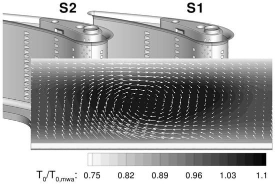
Figure 7.
Typical residual swirl and temperature profile at the exit of a lean-burn gas turbine combustor [75].
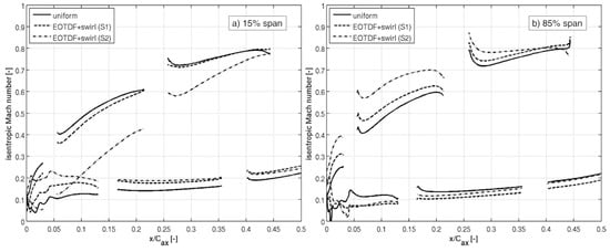
Figure 8.
Effect of residual swirl on isentropic Mach number distribution at 15% of blade span (a) and at 85% of blade span (b) of a high-pressure turbine vane [75].
Griffini et al. [76] studied the clocking effects of inlet non-uniformities by means of CHT simulations. Turbulence was modelled by using a tuned version of the approach by Walters and Cokljat [77] as in [72,75]. Hot spot migration through the vane depended on the interaction between the residual swirl, its clocking, and secondary flows. The configuration where the swirl was aligned to the vane leading edge turned out to be the most harmful, leading to hot spots on both pressure and suction sides. Salvadori et al. [78] studied the impact of a residual swirl with a superimposed hot spot [37,65,66] on the adiabatic effectiveness maps generated by a platform cooling device. The numerical approach was validated against experimental data obtained for a uniform profile, then non-uniform cases were studied. Salvadori et al. [78] showed that the development of the horseshoe vortex was governed by the presence of the inlet swirl, which, in the presence of cooling holes, also altered blade temperature values below of the span. The redistribution at higher spans of the coolant associated with the development of secondary flows was shown by means of streamlines and stagnation variable maps. Furthermore, a local variation in the adiabatic effectiveness values on the end-wall in the range – was evidenced with respect to the uniform inlet case. Results obtained by Charbonnier et al. [74], Salvadori et al. [78] and Griffini et al. [76] effectively substantiated the impact of residual swirl and hot spot migration of the aerothermal performance of a fully cooled high-pressure turbine vane.
Several activities were performed in a test rig designed by Cubeda et al. [79] (see Section 3.2.1) to analyze the redistribution of the hot flow in the cooled vane passage in the presence of a strong residual swirl. Babazzi et al. [80] used Pressure-Sensitive Paint (PSP) to evaluate film cooling performance and an oxygen concentration probe to track cold streak migration, and demonstrated that in the investigated configuration, low-coverage areas appeared on the suction side due to swirl-induced alterations of the streamlines. The presence of a strong residual swirl modified the stagnation line shape and position, thus altering vane load distribution [80] and the heat transfer coefficient maps [81]. Moreover, the unsteady nature of the swirling flow generated a fluctuating map of adiabatic effectiveness that was not represented by the time-averaged one. The swirling flow was also responsible for the redistribution of the cold streak downstream of the vane, with a specific pattern associated with the clocking between the residual swirl and the vanes. Film cooling effectiveness was also analyzed by [82] through RANS simulations, which were not able to correctly simulate coolant traces due to the high mixing associated with the presence of the swirl, coherently with what was found by Cubeda et al. [83]. However, RANS was able to qualitatively evaluate heat transfer coefficient maps if compared with the available experimental data. Bacci et al. [81] also found experimentally that the hot streak migration was influenced by the inlet swirl, resulting in a radial displacement of the hot flow. That behavior was coherent with what was found for linear cascades by Griffini et al. [76].
In recent work by Adams et al. [84], the effect of a combined hot streak and swirl profile on a cooled one-and-a-half stage was studied. The authors performed an experimental analysis at the OTRF using a lean-burn combustor simulator designed by Hall et al. [85], Hall and Povey [86]. The design and commissioning of the one-and-a-half stage was reported by Beard et al. [87]. They performed a detailed numerical simulation by including of the annulus thanks to the blade count ratio of 2:3:1. The comprehensive analysis performed at the OTRF allowed for understanding the driving mechanisms for the alteration of vane and blade aerodynamics. While the high-pressure vane aerodynamics were predominantly driven by the inlet swirl, which causes variations in loss distributions and vane exit flow stagnation properties, blade aerodynamics were driven by the inlet temperature profile thanks to the variation in incidence angle (up to ) associated with the segregation effect. The intermediate pressure vane is affected to a smaller degree, but it was found that vane loading and secondary flow structure were altered anyway.
2.7. Turbulence Intensity and Length Scale on Turbine Inlet Section
The analysis of turbulence levels on the inlet section of the high-pressure turbine has been the subject of discussion for many years. Researchers now agree that a “high” turbulence intensity is present downstream of the combustion chamber even if the actual values of turbulence fluctuations and their length scales are emerging only from recent studies thanks to high-fidelity computational fluid dynamics.
Radomsky and Thole [88] provided a review of the existing literature data and found that the turbulence level downstream of gas turbine combustion chambers was usually between and . Nevertheless, only a few bits of information were present concerning the turbulent length scale, and Radomsky and Thole [88] indicated an interval between and times the vane pitch. They also demonstrated experimentally that the turbulence level of the flow at the turbine entrance did not decay significantly through the vanes and remained high. Local increases in the turbulent kinetic energy had been observed in the regions characterized by strong curvature of the streamlines (e.g, outside of the boundary layer, on the suction side, near the stagnation points). Moreover, they concluded that high turbulence intensity within the vane passages caused both an early transition of the boundary layer and the enhancement of the heat transfer coefficient [88].
A significant contribution in understanding the characteristics of turbulence on the interface between combustor and turbine has been given by Cha et al. [89]. They studied experimentally a test rig including actual engine hardware, composed by a Rich–Quench–Lean (RQL) annular combustion chamber with a downstream row of nozzle guide vanes. The turbulence intensity map measured on the combustor/turbine interface plane demonstrated that extended zones with high turbulence intensity, up to , were present in the central part of the channel height. Also, the distribution of turbulence length scale (normalized with the vane chord) located on the same measurement plane was characterized by peaks up to , while extended zones at about were observable.
Similar results were obtained by Notaristefano et al. [90], who found turbulence intensity levels up to . Moreover, Koupper et al. [91] performed a LES of a hot streak generator representative of a lean-burn effusion cooled combustor for aero-engines and found turbulence level peaks between and that were located in the middle of the channel. Those turbulence levels were confirmed by Zarrillo [92] when simulating the test case described by Insinna et al. [23] and studied by Insinna et al. [24]. In fact, Figure 9 shows that high turbulence levels (up to ) are located at the turbine inlet section with a core region located close to the mid-span. The latter conclusion is coherent with the map of axial vorticity reported in Figure 3, where the highest vorticity values generated by the swirler in a lean-burn configuration are located close to the the center of the combustor.
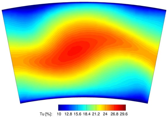
Figure 9.
Distributions of turbulence intensity on the combustor/turbine interface plane [92].
2.8. Wake/Blade Interaction
In the absolute frame of reference of a turbine or a compressor stage, the wake is seen as a velocity defect with respect to the main flow. According to some studies [93,94], the velocity deficit was mixed out, resulting in mixing losses. Considering a 2D inviscid configuration, a correspondence between wake mixing and stretching/compression and the unsteady losses was found. In the compressor stages, the wake stretched because of the suction side main flow velocity, while in the turbine row, the wake was compressed. According to Kelvin’s theorem, the velocity defect in a stretched wake should be smaller than in a compressed one and the mixing losses are lower in a compressor than in a turbine.
Even if these considerations are consistent with a 2D inviscid case, it is not plausible to rely only on them when studying turbomachinery flows. Due to the complexity of highly loaded blades, a wake could be stretched and then compressed in the same vane or blade passage. Furthermore, the 3D and the viscous effects cannot be neglected and a wider horizon of test cases should be considered. Following the classical velocity triangle decomposition reported in Figure 5, the circumferential velocity non-uniformity caused by the wake is responsible for the generation of a slip velocity vector which governs the wake redistribution into the passage (see Section 2.5). In fact, the wake impinges on the blade pressure side due to the shape of the velocity triangles but is transported toward the blade suction side since the wake flow is characterized by the slip velocity vector in the relative frame of reference. When the wake flow reaches the suction side, it spreads out, interacting with the incoming flow that initially decelerates and then accelerates. As a consequence of this mechanism, the boundary layer structure is modified and two opposite pressure fluctuations (on the suction and pressure sides) occur.
Some authors [95,96] evaluated the unsteady lift on a blade row subjected to wake passages. When the wake flow impinged on the blade, the incidence was negative and the blade lift decreased. This meant that the amplitude of the unsteady fluctuations of the pressure levels on the blade was enhanced, leading to higher acoustic effects. Boundary layer transition was another important effect of the wake/blade interference. When the wake impinged on the blade suction side, a turbulent spot was created inside of the boundary layer. Some studies [97,98] demonstrated that the turbulent spots were stretched while running downstream on the suction side and in the end, they collapsed into a turbulent boundary layer. Moreover, the zones crossed by the turbulent spot presented a quasi-laminar boundary layer which was resistant to transition. This effect was explained by the higher shear stress levels present in these zones. The wake-induced transition is currently, together with the bypass transition, the main transition mode in gas turbines and affects the profile losses by a factor of about .
A numerical study on the wake/blade and the wake/wake interaction performed by Hummel [99] by using an appropriate time–space discretization allowed for simulating the behavior of the von Karman vortex from both the blade rows and showed that in a turbine stage, the vane vortex street was tuned by higher harmonics (between the 6th and the 9th) of the blade passing frequency. According to that result, an unsteady simulation based on the “phase lag” assumption and the Fourier decomposition method [100] could catch the vortex shedding if a high number of harmonics was considered (see Section 3.3.5 for more information). Furthermore, Hummel [99] studied the effects of the temperature distortions in the vortex street individuating the “energy separation” phenomenon. An extensive description of that loss mechanism can be found in [101,102].
Miller et al. [103] studied experimentally a high-pressure transonic turbine stage and demonstrated that the exit flow was dominated by the tip leakage flow, the hub passage vortex, the trailing edge shock system, and the wake. They identified two important periodic changes in the blade exit flow field. The first one was a vane periodic fluctuation in the flow field close to the blade hub and was caused by the pooled vane wake segments, which were generated by the blade chopping, aided to a lesser extent by the secondary flows of the vane. Due to its effect, the blade trailing edge shock close to the hub and the low stagnation pressure region associated with the hub passage vortex periodically disappeared. The second fluctuation had the same periodicity but was weaker and was distributed over the entire span. The Mach number and the stagnation pressure fluctuated at the same blade and vane relative phase and this effect seemed to be caused by the vane/blade shock system, by the potential flow interaction, and by the chopped wakes that did not move towards the hub.
The time-resolved measurements performed by Schlienger et al. [104] at the blade exit of a two-stage axial turbine partially confirmed the existence of the first periodic fluctuation individuated by Miller et al. [103]. In fact, they concluded that the unsteady flow field at the blade hub exit was mainly driven by the interaction between the blade passage vortex and the secondary flow structures coming from the vane. Concerning the interaction between the wake chopped by the blade and the hub passage vortex, they individuated an interesting mechanism in which the wake was rolled up into the secondary structure, which could lead to the unsteady effect described by Miller et al. [103]. In the transonic and supersonic turbine stages, the oblique shocks that were generated at the vane and blade trailing edges contributed to enhancing the complexity of the unsteady flow field. While the vane trailing edge shocks interacted with the blades, the shocks from the blade trailing edge were affected by the chopped vane wake. Furthermore, both were responsible for an induced boundary layer transition on the respective adjacent blades, then modified the heat transfer rate, while their reflections travelled both upstream and downstream of the stage.
Finally, in aero-engines at cruise conditions, the Reynolds number can be reduced down to a value of ≈30,000, thus leading to a possible relaminarization of boundary layer in low-pressure turbine stages. Current trends in low-pressure turbine airfoil design aim at developing ultra-high-lift solutions that increase the risk of relaminarization, which is responsible for an increase in profile losses. The already mentioned “negative jet” effect periodically energizes blade suction side boundary layer, promoting the transition of the laminar separation bubble to a turbulent state. However, residual losses can be individuated, leading researchers to develop methodologies based on synthetic jets and plasma actuators to completely suppress them.
Summarizing, wake/blade interaction in turbomachinery depends on Reynolds number, outlet isentropic Mach number, diffusion ratio, and blade count and requires high-fidelity numerical methods and highly detailed boundary layer measurements to be studied. However, a detailed description of unsteady vane/blade interaction in low-pressure turbine stages is out of the scope of this paper. Information on this topic can be found in the selected contributions by Qiu and Simon [105], Stieger et al. [106], Hodson and Howell [107], Suzen and Huang [108], Sarkar and Voke [109], Mahallati et al. [110], Mahallati and Sjolander [111], Michelassi et al. [112], Pichler et al. [113], Marconcini et al. [114], Simonassi et al. [115], Lopes et al. [116].
2.9. Shock/Blade Interaction
The shock system within the vane/blade gap of a turbine stage was well-described by Dénos et al. [117]. Considering an experimental and numerical campaign conducted on the CT3 test case at Von Karman Institute for Fluid Dynamics (BE), they observed that the largest pressure fluctuations on the blade were situated at the blade leading edge, where the left shock running from the vane hit the blade and then moved towards the pressure side. The numerical campaign confirmed the obtained results, thus showing that depending on the vane/blade relative position, there were expansion waves and/or reflecting oblique shocks. In fact, an unsteady converging–diverging nozzle was periodically created by vane/blade aerodynamics in the gap region, which was responsible for the described behavior. The authors observed that the shock system produced fluctuations of relative stagnation pressure of amplitude and (if compared to the design values) at the blade inlet and on the blade crown, respectively. Furthermore, they concluded that in these configurations, vane wakes were distorted by the shock system but did not have a relevant effect on the observed stagnation pressure fluctuations.
In successive studies by de la Loma et al. [118] and by Paniagua et al. [119], the shock reflection mechanism was described in more detail. The left-running shock from the vane impinged directly on the blade and a reflected shock appeared, followed by expansion waves. During the blade movement, the reflected shock grew in intensity and moved towards the adjacent vane suction side (a phenomenon called “shock-sweeping”). The right-running reflected shock reached the blade and merged with the compression waves close to the leading edge. Furthermore, the wake originating from the vane interacted with the right reflecting shock and was chopped by the passing blade. In this configuration, pressure fluctuations wider than the time-averaged pressure values were experimentally found by the authors. Concerning the heat transfer, its behavior was associated with the unsteady flow field for the shock-induced boundary layer transitions on the vane suction side and on the blade crown. Furthermore, the blade height for the highly 3D blades was an important parameter for the heat transfer evaluation, since the shock strength and inclination depended on these parameters.
Miller et al. [120,121] performed an experimental and numerical simulation of a one-and-a-half stage with and without the downstream blade. They showed that at the nominal working conditions, the interaction between the vane trailing edge shocks and the blade was about 10 times stronger than the wake/blade interaction. Furthermore, they observed that as the vane trailing edge approached the blade leading edge, the oblique shock grew stronger, since an effective throat area occurred. This effect reduced its strength while the shock moved on the blade suction side, while another peak in shock intensity could be observed when it reached the blade leading edge. Concerning the presence of the second vane, it did not seem to affect the pressure field before the blade geometrical throat area. However, each vane experienced a new deterministic frequency and the pressure field on the blades showed a new fluctuating component, whose frequency corresponded to the difference in the upstream and downstream vane passing frequencies. This result was consistent with the one obtained by Li and He [122].
Figure 10 helps visualize the shock system occurring in a transonic high-pressure turbine stage [117,119,120,121]. Five different relative positions between vanes and blades obtained from a 2D simulation performed by Ottanelli [123] using the in-house solver HybFlow equipped with phase-lagged boundary conditions for multiple perturbations [124,125] are reported. The numerical test case reproduces the mid-span of the CT3 test case described by de la Loma et al. [118] with modified mesh and numerical sampling frequency, and allows for visualizing the shock system through numerical Schlieren visualization. A detailed description of the shock system is as follows:
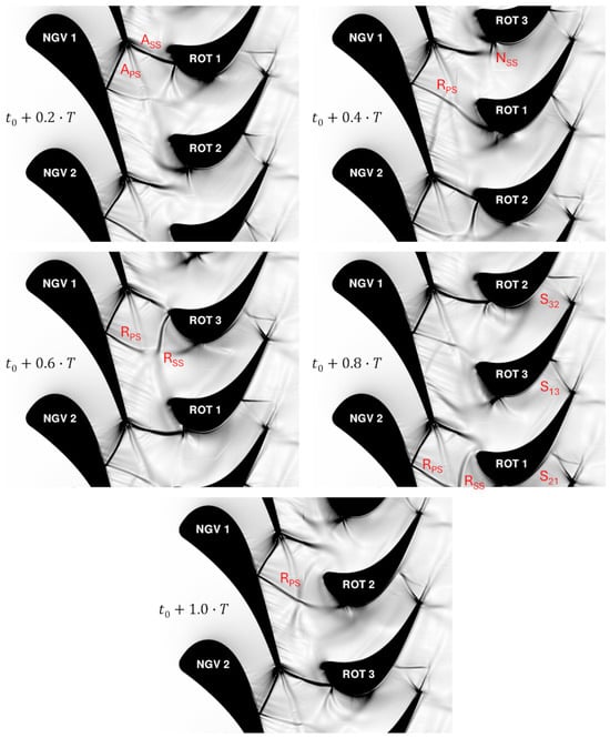
Figure 10.
Numerical Schlieren visualization of the shock system occurring in the CT3 high-pressure turbine stage at mid-span (adapted from [123]).
- At time , the oblique shocks and (both generated from vane ) are visible. Shock impinges on the suction side of vane and shock impinges on the suction side of blade close to the leading edge (and is weakly reflected).
- At time , the oblique shock is reflected through the axial gap () and impinges on blade (which, in the meantime, moves in the direction of rotation). Moreover, the shock interacts with blade , generating locally the normal shock and causing a local instability in the boundary layer.
- At time , the shock does not reach any blade, while a new reflected shock () appears, originating from thanks to the “shock-sweeping” mechanism. The reflected shocks along with the oblique shocks generate a region delimited by high-density gradients in the vane/blade gap.
- At time , a configuration similar to the one occurring at time occurs, but with a weaker intensity of .
- At time , a configuration similar to the one occurring at time occurs, but without the formation of the normal shock.
As can be observed, the same shock structures periodically appear depending on the relative position between vanes and blades. It is also interesting to underline that the oblique shocks generated from blade trailing edges depend on the vane/blade relative position, thus demonstrating the periodic formation of converging–diverging nozzles in the inter-stage gap [117]. Looking at the numerical Schlieren visualization at time , shocks , , and are characterized by different intensities and their reflection on the blade suction side is not always present, thus demonstrating their unsteady nature. Similar structures are visible at the other time frames, along with density gradients associated with the shock impingement from vanes or blades.
A dedicated study aimed at controlling shock angle and fluctuations was described in Saracoglu et al. [126]. Unsteady blowing of coolant flow was used to interact with both the vortex shedding and the corresponding oscillation of the shocks originated by the vane trailing edge at different Reynolds and isentropic outlet Mach numbers. It was demonstrated that detrimental effects of the shock waves were reduced with pulsating cooling. Saracoglu et al. [127] also demonstrated that it was possible to individuate an optimal coolant flow rate that minimized the accumulated shock and profile losses, although negligible differences were found by means of numerical simulations between pulsating cooling and the corresponding steady cooling.
2.10. Clocking Effects between Blade Rows
Since the wake is usually not completely mixed out, its effect on the downstream rows should be considered. In a multistage gas turbine, the effects of the vane/vane and the blade/blade interactions could be as important as the vane/blade interaction. Generally speaking, the intensity of the blade/blade interaction depends strongly by the blade count ratio. Moreover, He [128] demonstrated that a non-uniformity with a long wavelength decayed at a slower rate in the axial direction.
If two consecutive blade rows have the same blade number, the blade/blade time-averaged flow field has a periodicity of a blade pitch. That situation represents the maximum clocking effect. The phenomenon is weakened if two consecutive blade rows have a blade count for which the only possible periodicity is represented by the complete ring. In that case, the circumferential wavelength of the blade/blade fluctuations is equal to the full periodicity, and there is no spatial periodicity over one blade pitch. Therefore, some assumptions will be necessary when performing a single passage simulation or an experimental analysis (see also Section 3.3).
The clocking effects in a one-and-a-half high-pressure turbine stage test case were studied by Li and He [122]. They observed that on the blade surface, the nonlinear interaction between the two fundamental frequencies generated sub-harmonic fluctuations which were linear combinations of the blade passing frequencies. In this case, the upstream and downstream vanes influenced the magnitude of the sub-harmonic components. Concerning the vane/vane interaction, when the number of blades was different, a non-periodic flow was induced in both the vanes. Looking at the unsteady flow around the vane, neither a constant magnitude nor a constant phase shift was visible, while an unsteady forcing variation of about three times in magnitude for the second vane was observed. Varying the second vane number, the authors found that the phasing between the first vane wake and the blade unsteadiness was a function of the vane/vane clocking position. These results underlined the importance of an accurate choice of blade clocking during the design phase, coherently with the results obtained by Hummel [99].
A numerical simulation of a two-and-a-half compressor stage test case, using a nonlinear harmonic solver, was performed by He et al. [129]. In this case, the upstream and downstream vanes had the same number, while the blade did not. He et al. [129] observed that the vane clocking did not affect the time-averaged polytrophic efficiency distribution, while the blade/blade interaction was responsible for a non-periodic fluctuation higher than , both in subsonic and in supersonic conditions. Furthermore, the time-averaged distribution of the polytrophic efficiency showed four peaks generated by the difference in the blade number (17 and 21, respectively). The authors also increased the blade number of the first blade row to a value equal to that of the second blade row and observed an efficiency fluctuation of in the transonic case, while in subsonic conditions, it was about . Furthermore, the shape of the fluctuations in these cases was not comparable, suggesting a qualitatively different blade/blade interaction mechanism in a transonic flow when compared to that in a subsonic flow.
Eventually, considering a transonic compressor, the interaction between the wake generated by the upstream blade and the shock system occurring downstream enhances the global losses. In fact, mixing losses are higher when they are subjected to adverse pressure gradients [13]. Furthermore, the shock strength is tangentially non-uniform, then the blade/blade clocking influences this mixing loss mechanism.
2.11. The Role of Unsteadiness in the Generation of Losses
The global effects of the phenomena presented between Section 2.2 and Section 2.9 on the generation of unsteady losses and on the heat transfer must be studied and a parameter to quantify the flow losses in an unsteady case should be defined. He [130,131] studied the entropy/ decoupling mechanism in turbine stages and showed that the stagnation pressure was representative of the losses only in a steady environment. In fact, considering the energy equations reported in Equation (5), it can be observed that entropy generation is associated with stagnation pressure in steady adiabatic cases only.
In fact, in a steady adiabatic case, an entropy rise on the streamline is always associated with a stagnation pressure decrease, while considering an unsteady inviscid case, pressure variations in time influence stagnation enthalpy. He [130,131] performed an unsteady inviscid calculation of a turbine blade row subjected to incoming wakes (modelled as an inlet boundary condition) and compared the pitch-wise time-averaged entropy and stagnation pressure variations. This study evidenced that in some pitch-wise positions, corresponding to the vane trailing edge far form the blade surfaces, entropy and were decoupled. It was concluded that in an unsteady viscous situation, stagnation pressure variations provided some information on the global losses but were also affected by the Euler flow field far from the blade surfaces.
The experimental and numerical analysis performed by Payne et al. [17] proved that the primary flow entropy increase was the main source of losses. Furthermore, a large fluctuation of the time-resolved stage efficiency was observed, underlying the importance of the vane phase on the unsteady loss entity. Pullan [16] confirmed this result by comparing the data obtained from a steady and an unsteady simulation. The steady simulation generated less losses when compared with the unsteady one. Therefore, an accurate unsteady simulation of the final configuration of a newly designed turbine stage must be performed in tandem with a steady simulation.
A detailed description of loss mechanisms associated with unsteady fluctuations in gas turbines is out of the scope of the present paper. An exhaustive analysis of turbine losses is available in the work by Denton [13].
2.12. Aerodynamic Instability and Aeroelastic Effects
Several unsteady disturbances are presented in this paper and their effects on the unsteady flow field are evidenced with the support of relevant studies. As already pointed out for the wake effect on the blade load, the mechanical response to the unsteady pressure fluctuations may cause the turbine to fail. If no dumping mechanism occurs, an excessive stress level can be present if the frequency of the unsteady fluctuations coincides with a particular vibration mode of the blade.
The aeroelastic instability effects on the turbine residual life must be taken into account during the design process. The most important aerodynamic sources of instability are represented by the wake/blade interaction, the incidence variation, and pressure fluctuations. The fundamental interference wavelength caused by these phenomena is a function of the geometrical parameters and of the boundary conditions. Once the blade number and the rotational speed are known, the deterministic frequencies of fluctuation can be determined and compared with the vibration modes of the mechanical parts of the turbine. Usually, the instability must have a frequency which is not a multiple of the resonant frequency of the blade. Even if it is possible to obtain good results at the design conditions, the problem may arise considering off-design conditions (e.g., the startup and the shutdown of the turbine). For this reason, several researchers developed numerical methods to investigate this aspect of the compressors and turbine aerodynamics [132].
Concerning the stochastic sources of vibration, the blade flutter is a self-excited aeroelastic instability phenomenon. When the blades are excited by the above-mentioned sources, they tend to vibrate with small amplitude at their natural modes. In some conditions, the unsteady forces resulting from this vibration periodically transfer some energy to the blade and the vibration amplitude increases. If no mechanical dumping occurs, the flutter instability can lead to blade failure. To evaluate correctly the risk of failure, the phasing between the aerodynamic sources and the blade vibration must be considered. In Equation (6), is the vibration displacement, is the vibration velocity, is the force applied from the fluid to the blade, and are the amplitudes of the oscillation of the displacement and of the force, respectively, is the pulsation of the oscillation, is the phase shift, and W is the work done by the fluid on the blade.
It can be assumed that both of them are sinusoidal with the same periodicity but with a different phasing. Using this assumption, the effect of the higher-order harmonics on the net energy transfer is neglected. The entity of the work done W can be calculated, the flutter instability being activated when the work is positive.
Considering Table 1, there are three important self-excited aerodynamic instabilities to be discussed, namely vortex shedding, shock oscillation, and rotating stall. Since shock oscillation has already been extensively discussed in Section 2.9, its description is not going to be repeated here.
The vortex shedding is an important source of profile losses for turbines blades with a thick trailing edge. The development of vortex shedding has been extensively studied by means of experimental measurements by Sieverding et al. [133] along with the evaluation of the pressure distribution at the trailing edge of a turbine vane by using turbulent kinetic energy contours. To correctly evaluate this phenomenon, an unsteady simulation is necessary to correctly calculate the trailing edge static pressure level. The vortex shedding has a short wavelength and its frequency, in the case of an undisturbed flow, is connected to the boundary state and the trailing edge dimension. Hummel [99] demonstrated that in turbine stages, vortex frequency could be fixed at the higher harmonics of blade passing frequency. Nevertheless, the acoustic vibrations and the blade oscillations affect the vortex frequencies, acting as exciting sources. Then, its correct evaluation with the numerical tools is still an open problem that involves high-fidelity numerical methods and mesh deformation tools.
The rotating stall is an important unsteady phenomenon that affects the compressor performance and its residual life [134]. This circumferential instability produces relevant blade vibrations and is the precursor of the surge problem [135]. The basic activation mechanism of the rotating stall has been described by Emmons et al. [136] and is briefly reported here. Considering the blade row of a compressor stage visible in Figure 11, represents the nominal velocity profile at blade inlet section and is a local off-design condition for which the velocity vector hits the blade with a positive incidence. Due to the small thickness of the leading edge, the local acceleration of the flow, and the positive pressure gradient that occurs across the compressor stage, the boundary layer that is developing on the suction side of the blade becomes unstable and eventually separates. A massive separation of the boundary layer creates a recirculation region that closes the passage (highlighted in red) and obliges the incoming flow to modify its trajectory. Therefore, the incidence on blade becomes negative due to the direction of vector and, on the contrary, the incidence on blade becomes strongly positive due to the direction of vector . As a consequence, passage starts opening and a new stall region (also called “cell”) develops in the passage . Usually, two consecutive passages are subject to the rotating stall phenomenon. Also, in the relative frame of reference, the stall moves in the opposite direction of the rotational speed but with a lower intensity. Since a typical stall velocity is about of the rotating velocity, in the absolute frame of reference, the stall rotates aligned with the direction of rotation.
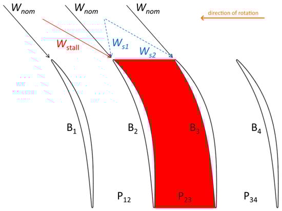
Figure 11.
Rotating stall mechanism in axial compressors.
He [137], He and Ismael [138] performed several unsteady simulations to study rotating stall characteristics. The unsteady simulation of two compressor stages with different blade count showed that the number of stalled vanes, the circumferential wavelength, and the stall rotating speed were dependent on the blade count. A compressor stage with a spatial periodicity of half an annulus showed two stalled cells, but if the periodicity was the whole annulus, only one cell was stalled. Then, the stall pattern depended on the beating frequency of the vane/blade disturbances. However, the results obtained for a transonic flow were not extendable to subsonic compressors for the difference in the pressure fluctuations running upstream of the blade row.
A detailed discussion of the stall and surge phenomena is out of the scope of this paper. More information can be found in Day et al. [134], Greitzer [139,140], and Stenning [135].
3. Component Interaction Analysis
The increasing demand for high-efficiency gas turbines makes the study of component interaction of paramount importance. In fact, the interactions can either be a source of unexpected performance degradation or lead to reduced component life. For these reasons, researchers started investigating the aerothermal phenomena involved in compressor/combustor (Section 3.1), combustor/turbine (Section 3.2), and vane/blade (Section 3.3) interactions to provide useful information for gas turbine designers.
3.1. Compressor/Combustor Interaction
The study of compressor/combustor interaction is particularly important for annular and can-annular combustors, which are typically used in aero-engines. They are characterized by compact geometries to reduce losses, but they also subject to increased aerodynamic instabilities related to pre-diffuser/combustor layout. This is especially true in lean-burn combustors, where dilution ports are reduced and about of the overall air flow rate passes through the burners.
The combustor inlet flow is characterized by radial and tangential flow distortions, large-scale fluctuations (wakes), and residual swirl (that increases with flow deceleration), all of them generated by the high-pressure compressor stage. The pre-diffuser and the diffuser may not be able to completely suppress those non-uniformities, thus increasing the risk of also having non-uniformities in the primary combustion zone. Radial and tangential non-uniformities are responsible for an unbalanced flow distribution on the entire burner entry section, thus generating a high sensitivity of the combustor performance to the upstream conditions and the unequal distribution of the flow on all the burners, which affects the flame behavior. Furthermore, the coherent temporal fluctuations associated with blade wakes and separations may alter the local stoichiometry, leading to potential problems with emissions control and to enhanced combustion instabilities.
The main objective in the efficient design of the interaction region between the compressor and the combustor is to increase the performance of the “air distribution system” to the combustor, which is composed of the Outlet Guide Vane (OGV) and the pre-diffuser. In particular, a reliable design should be able:
- to ensure uniform air feeding to burners;
- to ensure effective air redistribution to the combustor walls;
- to increase pressure recovery across the pre-diffuser, avoiding its stall;
- to reduce overall stagnation pressure losses;
- to avoid unexpected working conditions or instabilities of the reacting flow due to disturbances coming from the compressor.
Most of the currently available research about the compressor/combustor interaction topic is based on experimental tests. An experimental test rig for the study of compressor/combustor interaction typically contains the last stage of high-pressure compressor (blade and OGV), the pre-diffuser, the dump diffuser, and the combustor. An example of such a configuration can be found in the work by Cha et al. [26], where the high-pressure vane of the turbine module was also present. Ford et al. [141] studied experimentally the impact of compressor exit conditions on fuel injector flows. They demonstrated that at the exit of the pre-diffuser, non-negligible velocity variations (between and of the averaged value) were present, which propagated through the injector and were responsible for non-uniform velocity profiles in the primary zone. Furthermore, measurements performed at the injector exit plane evidenced the presence of a flow fluctuation whose frequency was associated with the high-pressure compressor blade passing frequency. The amplitude of that oscillation was higher than the one associated with the aerodynamic instability of the swirler, thus generating a risk of enhanced combustion instability.
In a numerical study, Walker et al. [142] showed how a joint optimization of the OGV and of the pre-diffuser allowed for designing a geometrical solution that prevented diffuser stall while working in the unstable region of a diffuser chart. In fact, it was possible to obtain an increased area ratio of the pre-diffuser (from conventional up to ) with the same length and without separation, thus demonstrating that the performance of a diffuser in a “turbomachinery environment” can be better than in a “clean environment” thanks to the presence of high free stream turbulence and wakes. A similar result was found by Stevens et al. [143], who concluded that when the OGV was positioned close to the pre-diffuser, the outlet velocity profile was more stable than in the case of a fully developed inflow.
Later, Walker et al. [144] studied the impact of the dimension of the dump gap d between the pre-diffuser and the combustor cowl on the static pressure contours at the pre-diffuser exit. They found that considering a “short” dump gap (, where h is the pre-diffuser exit radial extension), the blockage of combustor cowl stabilized the flow inside the pre-diffuser but also induced flow distortions. On the contrary, considering a “long” dump gap (), there was no effect on pre-diffuser aerodynamic stability but the pressure field at the injector inlet section was almost uniform. Stevens et al. [143] suggested a length for d between 3 and 4 OGV chords for the wakes to decay significantly.
Considering that the flow in that portion of the combustor is subsonic, Walker et al. [144] evaluated the pulsating frequency of the flow between the high-pressure compressor blade and the OGV, thus demonstrating that the blockage effect of the combustor cowl travelled upstream of the OGV (at least for ). In fact, the pressure variation caused by the cowl suction was larger than the OGV potential disturbance and was approximately equal to of the blade stagnation pressure rise, which was enough to change the blade characteristic. Therefore, a dump gap with was also beneficial for the last blade row of the high-pressure compressor.
A detailed experimental analysis of a configuration similar to the one reported in [144] but equipped with both a clean and a strutted OGV/pre-diffuser system was presented by Walker et al. [145]. Thanks to the usage of several experimental techniques, light was shed on the performance of the OGV/pre-diffuser system caused by both the high-pressure compressor blade and the presence of lean-burn injectors. The performance of the high-pressure compressor blade was not influenced by both the radial struts and the high mass flow rate associated with lean-burn injectors. On the contrary, losses through the OGV increased up to in the presence of radial struts, and the OGV exit section was characterized by secondary flows and high turbulence levels that were responsible for unsteady flows interacting with the lean-burn injectors. It is also worth mentioning that the implementation of PIV in such a realistic environment was a significant improvement with respect to the typical approaches.
From a numerical point of view, the coupled simulation of the compressor and the combustor is complicated by the different flow characteristics of the two components. In fact, a compressor is characterized by moving blades, high Mach number, and wall-bounded, non-reactive, single-phase flows. On the contrary, a combustor is characterized by stationary components, low Mach number, large-scale coherent flow structures, and reactive multi-phase flows with high heat release. To couple these two elements is numerically complex both using a single solver and two solvers coupled at the interface. Karki et al. [146] proposed a decoupled method to study the pre-diffuser and the combustor that allowed for evaluating the static pressure recovery in agreement with the experimental data within an error of . Furthermore, 3D simulations evidenced that the flow distribution through the swirlers is non-uniform, as confirmed later by Ford et al. [141].
An integrated approach to compressor/combustor interaction analysis using Computational Fluid Dynamics (CFD) was proposed by Kannan and Page [147] for steady coupling and later extended to unsteady coupling in [148]. The proposed methodology was in line with the ones presented by both Collado Morata [149] and Insinna et al. [150] for combustor/turbine interaction analysis, and allowed for studying the unsteady flows through a high-pressure compressor stage, a pre-diffuser, and a combustor in cold flow conditions with a multi-solver approach. Results obtained with the unsteady simulation confirmed the presence of non-negligible non-uniformities at the pre-diffuser exit section caused by flow exiting the high-pressure compressor components. Furthermore, the unsteady multi-solver approach demonstrated an increase in accuracy with respect to both the steady approach and a standalone simulation when comparing the tangentially averaged radial distribution of static pressure at the pre-diffuser exit section with the available experimental data.
A more sophisticated methodology for compressor/combustor interaction analysis by using a multi-solver approach was proposed by Schlüter et al. [151] and by Schlüter et al. [152]. A sector of an aero-engine was analyzed by coupling an Unsteady Reynolds-Averaged Navier–Stokes (URANS) simulation of the high-pressure compressor blades and OGVs and a LES of one sector of the annular combustor (including the pre-diffuser). Concerning the latter, since no inertial scale fluctuations could be derived by the URANS simulations, synthetic turbulence was added to prescribe appropriate boundary conditions for a LES. Obtained results were compared with the LES of the diffuser alone, thus demonstrating that the use of an integrated approach was necessary to correctly capture the axial velocity profiles inside the pre-diffuser. In fact, LES analysis of the pre-diffuser predicted a boundary layer separation which was not present in the coupled RANS/LES analysis. That result was coherent with what was found by Walker et al. [142]. Schlüter et al. [152] also analyzed the difference between a one-way (loosely coupled) and a two-way (fully coupled) approach, concluding that no effect was visible on the pre-diffuser performance, at least for the investigated case.
Soli et al. [153] performed a single-sector simulation of an RQL combustor coupled with a one-and-a-half stage axial compressor described by Denman [154]. The analysis was performed by coupling a density-based cell-vertex solver for the compression system with a pressure-based cell-centered solver for combustion simulation. The coupling algorithm was based on the presence of overlapping regions where the solution was continuously interpolated, thus allowing for a two-way synchronous communication between the sub-domains. The coupled simulation confirmed that incoming wakes induced distortions in the pilot flow field, changing the Precessing Vortex Core (PVC) behavior from single-frequency to broadband. As a general conclusion, it was demonstrated that selecting appropriate inflow boundary conditions for combustor simulations was of paramount importance, especially for compact combustors.
3.2. Combustor/Turbine Interaction
Combustor/turbine interaction analysis is currently one of the most challenging problems in turbomachinery analysis and design due to the inherent complexity associated with the study of low-Mach, reactive flows that expands through high-Mach, cooled flows. In this case, component interaction has an impact on key parameters for the efficiency, the specific fuel consumption, and the reliability of the gas turbine. Moreover, increased complexity is caused both by the possible use of hydrogen blends to reduce pollutant emissions [155] and by the expected change in the thermodynamic cycle to achieve a remarkable efficiency increase (theoretically in some configurations) through pressure gain combustion [156,157]. For these reasons, it is of paramount importance to design and manufacture realistic test rigs as well as to develop reliable numerical methods for combustor/turbine interaction analysis. In the present section, test cases available from the literature as well as numerical methods are reported and discussed.
3.2.1. Combustor Simulators for Combustor/Turbine Interaction Analysis
One of the aspects that makes combustor/turbine interaction a challenging topic in gas turbine research is the difficulty in dealing with an experimental campaign under actual working conditions. Experimental tests aimed at determining the temperature field at the combustor exit section on full-scale geometries at the machine design point are almost impossible and expensive. For these reasons, scientific papers that show realistic temperature profiles at the inlet of the high-pressure turbine are limited in number. Experimental data obtained during research projects allowed for validating numerical approaches that have been used to analyze the impact of the hot flow on turbine aerodynamics and heat transfer, sometimes in conjunction with residual swirl effects. An overview of the characteristics of the hot spot generators available in the literature as well as of the temperature field established downstream follows.
Povey et al. [32] showed the time-averaged temperature field measured at the exit section of a typical modern military engine, equipped with 20 burners. The thermal field was characterized by maximum temperature peaks over 2200 K, while the coldest regions, located near the hub and the casing, were even below 1500 K. Hot spots were present due to the tangential temperature gradients generated by the discrete number of fuel injection points and the presence of dilution jets [32] (no other information is provided by the authors about the type of combustion system). Strong radial gradients were caused by the liner cooling, even if the coverage provided by the coolant seemed to be insufficient to avoid high-temperature zones near the end-walls. The map shown in [32] allowed for noticing that for this particular case, the strongest tangential temperature gradients were located close to the hub.
Ong and Miller [158] showed a non-dimensional temperature distribution at the inlet of the high-pressure turbine experimentally measured by Mitsubishi Heavy Industries. In this case, the machine layout strongly influenced the temperature map. The machine was equipped with a can-annular combustor, where multiple flame tubes were positioned tangentially within an annular casing and were connected with the turbine inlet section through transition pieces. The well-defined hot spots were clearly visible in [158], where the cold spots generated by leakage of compressor exit flow close to the flanges of the transition pieces were also observable. It could be concluded that the can-annular combustor arrangement led to alternate “hot” and “cold” vanes.
Another representative stagnation temperature distribution downstream of a new generation lean-burn combustor for aero-engines was presented by Shahpar and Caloni [19]. The distribution of hot and cold zones was similar to the one reported in [32]. In this case, temperature gradients were mainly in the radial direction, due to the combustor liner cooling, but a marked hot spot was observable in the region at normalized pitch-wise coordinate between and .
Due to the difficulty of experimental testing in actual engine conditions, some research groups approach the problem of characterizing the turbine inlet temperature profile by means of tests under similitude conditions or through the development of “combustor simulators”. For both of these approaches, the flow is non-reactive and the exit temperature non-uniformity is studied by reproducing a hot spot through electric heaters or by means of the use of non-reacting tracers. For this latter approach, the mass transfer analogy is used to derive a non-dimensional temperature distribution.
Cha et al. [26] presented the experimental study of an RQL aero-engine combustion chamber tested in similitude conditions without fuel injection. The test rig included the full annular liner with burners and injection systems. Since a cold flow test was considered, CO2 was used as non-reactive tracer in order to reproduce the hot fluid distribution within the combustion chamber. The corrected CO2 concentration, obtained on a section positioned on the combustor–turbine interface plane, at which the boundary conditions were normally specified during the numerical simulation of the high-pressure turbine, was reported in Cha et al. [26]. A wavy-shaped hot spot was present on the investigated plane, with the maximum peaks located at about the mean radius of the channel. The cold zones were positioned along the end-walls and were extended near the casing.
Qureshi et al. [18] reported a stagnation temperature distribution measured downstream of a hot streak generator. The map covered two vane pitches and showed clearly the presence of well-defined hot spots, positioned centrally in the radial direction. In this case, the cold fluid covered the end-walls without presenting the tangential gradients evidenced by [19,26,32].
Hall et al. [85] performed the design and validation of a non-reactive combustor simulator with swirl and temperature distortions to be used in the Oxford Turbine Research Facility (OTRF). The challenges of correctly reproducing vortex instabilities (PVC or vortex breakdown) and the different heat release available in a non-reactive warm rig were taken into consideration during the design process. Flat vane swirlers was used to generate the residual swirl, while the radial temperature distribution was obtained by injecting cold flow close to the end-walls. A swirl/vane count of 20:40 was used based on the work by Kilik [159], thus allowing for simple numerical modelling by selecting only a portion of the annulus. In fact, the design the new geometry was performed relying on URANS calculations, which was demonstrated to correctly capture most of the vortex instabilities. Experimental data reported by Hall and Povey [86] demonstrated that the final design matches the target profile and conditions even in the presence of a PVC due to the non-oscillatory nature of the central recirculation zone. A generally good agreement was found between the experimental results and the URANS data available from the design phase, thus confirming that URANS was a valid tool for combustor simulator preliminary design. Recently, the original design [85,86] was modified and scaled by Amend et al. [160] for compatibility with the high-pressure operating conditions of the Engine Component Aerothermal Facility (ECAT) [161]. Numerical simulations were performed using different turbulence closures (namely [162], SST [163], and SSG RSM [164]) that demonstrated sufficient accuracy in the evaluation of flow profiles at the reporting plane without the vane when compared with the available experimental data, especially considering the model. The introduction of the vane caused an increase in the yaw angle due to the presence of the potential field, thus affecting the incidence on the vane leading edge. The “net circulation” effect was also analyzed, which was responsible for circumferential flow migration of vane pitches in the absence of a diffuser (which is not the ECAT case). A similar result was found by [24] for a combustor/turbine interaction analysis with a lean-burn configuration and an accelerating transition duct.
Koupper et al. [91], Bacci et al. [165,166], Koupper et al. [167], Krumme et al. [168], and Gövert et al. [169] developed an engine-representative combustor simulator dedicated to reproducing the expected turbine inlet profiles in terms of stagnation pressure, stagnation temperature, and flow field within the “Full Aerothermal Combustor–Turbine interactiOns Research” (FACTOR) project co-funded by the European Commission. The aims of the project were to develop both a trisector to be tested at the University of Florence (Florence, IT) and a full annular rig to be tested at DLR in Göttingen (DE).
Koupper et al. [91] presented the design of the real-scale trisector whose performance was compared with the one obtained using LES by a mono-sector, confirming that the central portion of the trisector was periodic. The isothermal operating point was selected for a Hot Wire Anemometer (HWA) measurement campaign and assessed by LES. The instrumentation of the test rig was also presented. Bacci et al. [165] presented the outcome of a numerical campaign oriented at describing the evolution of the flow field in the trisector for two different injector geometries, with and without a duct at the swirler exit section. The presence of the duct was necessary to reduce the dissipation of the vortex, thus maintaining enough similarity with modern combustors that were characterized by a non-negligible residual swirl at the exit section. Turbulence levels were also measured in a dedicated campaign by [166]. As a general result, it was concluded that the ducted configuration of the combustor simulator was able to match the target profiles in terms of stagnation values and flow angles at the turbine inlet section. Furthermore, a realistic turbulence level around was measured at the combustor/turbine interface section, even though a reduction of was measured on a plane positioned closer to the vane leading edge. Concerning the turbulence spectra at the interface plane for the ducted configuration, the first peak frequency was found at 350 Hz and is coherent with the PVC frequency of oscillation found by LES [91]. Turbulent timescales were also analyzed by Koupper et al. [167] by comparing HWA measurements with LES. It was found that a reliable evaluation of turbulent timescales would require at least 200 through flow, which was not compatible with the typical LES duration (usually ≈10 through flow). That was responsible for local errors up to . However, in the ducted configuration, LES and HWA agreed well with the timescale maps, and continuously increasing computational capabilities will help reduce local errors by means of a higher number of through flows. Based on the activity carried out on the trisector, the rotating rig was designed and manufactured and its main characteristics are described by Krumme et al. [168], where the main issues that were overcome are also reported. Gövert et al. [169] also performed an integrated simulation of the annular rig, even though only a sector of was considered thanks to the periodicity of the configuration, thus using a computational domain similar to the one used by Koupper et al. [170]. However, the selected approach was not scale-resolving and the obtained results were only meant to support the installation of the annular rig.
Several numerical simulations were performed using the data available from the FACTOR project. Andreini et al. [171] compared several numerical results obtained using commercial solvers and demonstrated the superior performance of Scale-Adaptive Simulation (SAS) [172] with respect to Shear Stress Transport (SST) [163] in the evaluation of the flow physics evidenced by using Particle Image Velocimetry (PIV). A dedicated study by Andreini et al. [173] about the impact of numerical modelling in the evaluation of the flow field occurring in the FACTOR combustor simulator confirmed that SAS was able to reproduce PIV data within at a reasonable computational cost. Moreover, two different approaches for film cooling modelling of the end-walls were compared in [171], concluding that the injection through discrete source terms [174] brought an increase in mixing between main flow and coolant, whose positive impact on the results was not fully justified by the increased modelling complexity. On the contrary, the increased computational effort associated with the simulation of the trisector instead of simulating only one sector under a periodic assumption was justified by the increased accuracy of the obtained results, at least in the configuration analyzed by Andreini et al. [171]. In fact, it must be pointed out that results obtained by [173] were in good agreement with PIV data also considering the central sector only.
Cubeda et al. [175] simulated the performance of the cooled high-pressure vane designed during the FACTOR project using the SST model as turbulence closure. Boundary conditions for the vane were taken on the combustor/turbine interface section using numerical data obtained during a previous numerical campaign [173]. Furthermore, an integrated domain was created to perform a simulation using SAS and ultimately verify the accuracy of the segregated approach. Concerning aerodynamics, no remarkable difference was found between the selected approaches, thus suggesting that a fully turbulent approach is an acceptable approximation for simulating only the vane. On the contrary, the decoupled approach with boundary conditions taken from a fully turbulent simulation of the hot streak generator generated unreliable results in terms of adiabatic wall temperature in the cooled case, with discrepancies up to 150 K. Only the integrated approach was able to reduce the error on radial temperature profile at vane exit by with respect to Reynolds-Averaged Navier–Stokes (RANS) simulations, and to reproduce coolant distribution. The same case was investigated further by [83], who confirmed the superior performance of the integrated approach through a more detailed comparison of the obtained results.
Concerning turbulence modelling, the typical under-prediction of turbulent mixing associated with the [162] eddy viscosity model could be limited by reducing the turbulent Prandtl number, but it requires a dedicated tuning that is not justified by the limited increase in accuracy. Andreini et al. [176] performed an analysis of modelling strategies for the prediction of hot streak generation in the FACTOR device including Large-Eddy Simulation (LES) and a study about the impact of turbulent Prandtl number variation. LES and SAS performed similarly on the selected mesh with respect to the experimental data, but SAS required times lower computational resources. Andreini et al. [176] also confirmed that the adiabatic homogeneous model by Mendez and Nicoud [177] allowed for accounting for the presence of effusion cooling with coarse grids, even if some limitations in reproducing the film temperature were found. Thomas et al. [178] simulated the same test case using a newly developed heterogeneous model for effusion cooling, concluding that it led to similar results as the validated homogeneous injection model. It is also relevant to underline that [170] demonstrated by means of integrated LES of the combustor simulator and the high-pressure vane that the potential effect induced by the vanes altered the mass flow rate redistribution and the turbulence level at the turbine inlet section, even though the temperature pattern was mostly unaltered. Recently, [179] performed integrated LES of the combustor simulator and of the high-pressure turbine stage, thus demonstrating its feasibility at academic and industrial levels. However, open issues remain and high-order numerical schemes as well as adaptive grid refinement may help understand some discrepancies between experiments and simulations, which are probably caused by coolant injection model and secondary flow development.
Recently, a test rig for combustor/turbine interaction analysis was developed in the frame of the “Smart Technologies” (STech) project that was coordinated by Baker Hughes (Florence, IT) and co-funded by the Region of Tuscany (IT). In this warm rig, both a real lean-premix combustor and a real high-pressure first-stage nozzle sector were designed to operate in non-reactive conditions. The development of the test rig was extensively described by Cubeda et al. [79]. The design mostly relied on RANS simulations of the uncooled rig and on LES of the combustor at engine scale, then cooling was implemented to increase the representativeness of the simulations. It was demonstrated by the preliminary experimental data that the final configuration was coherent with the target combustor exit profiles and with the periodic assumption for the central passage. The test rig was also used by [180] to successfully develop and validate a new experimental approach to retrieve reliable heat transfer coefficient and adiabatic wall temperature distributions simultaneously.
A summary of the most important facilities equipped with hot streak generators, installed in various laboratories, is given by Koupper et al. [91]. The maximum and minimum non-dimensional temperature peaks reached in each hot streak generator are reported, with the temperature non-dimensionalized with respect to the average value. Starting from the list available in [91], it is possible to draw the updated list of facilities reported in Table 2, with the corresponding project name being used if available.
Table 2.
Overview of main combustor/turbine interaction facilities.
Most of the temperature distortions were in the range except the LSRR case, which was characterized by a wider temperature interval . Among the listed ones, the most recent facilities were also the more representative of modern lean-burn combustors.
To summarize the qualitative and quantitative aspects emerging from the above-mentioned analysis of the temperature field, it is worth underlining the following conclusions:
- The most intense temperature gradients were mainly directed radially.
- Actual combustor geometries had remarkable tangential non-uniformities near the end-walls. The presence of tangential gradients in the center of the height of the channel was strongly dependent on the combustor architecture.
- Hot streaks coming from actual geometries were distorted. The same was not true for the profile shown in [18], coming from the hot streak generator presented in the work by Povey and Qureshi [37], where well-defined hot spots were present. Nevertheless, this consideration cannot be generalized to all the hot streak generators.
- In quantitative terms, the most representative hot streak generators aiming to reproduce aero-engine combustors are characterized by .
3.2.2. Numerical Methods for Combustor/Turbine Interaction Analysis
Experimental investigation of combustor/turbine interaction is complex and expensive. In fact, if the combustor is of annular type, it is difficult to reproduce an adequate periodicity between each sector without considering a considerable angular extension of the investigated section. This needs to handle high mass flow rates of reacting flow at high pressure. Therefore, such experimentation is difficult to sustain and the role of numerical predictions becomes crucial in understanding real working conditions of components.
A small number of scientific works are available in the open literature concerning numerical investigations of combustor/turbine interaction. One of the main reasons is probably the need for powerful computational resources, which have been developed only in recent years. Another reason is that the need for studying combustor/turbine interaction emerges because of the necessity to investigate in more detail the aerothermal aspects of the components’ operation. The need for these studies has been particularly strong in recent years, when emission regulations have become more restrictive and manufacturers have needed to work hard on combustion chambers, leading to the study of lean-burn combustion in aero-engines. The modern design of the combustion chamber is characterized by an aggressive aerothermal flow field, making necessary the simulation of combustor/turbine interaction in order to ensure component reliability.
The development of computer science and high-performance computing techniques in recent years has opened the way to numerical simulations for “multi-component” studies. The possibilities have been explored in the publications by Shankaran et al. [189] and by Schlüter et al. [190]. The latter described the development of a system aimed at simulating a gas turbine by jointly using the URANS approach for compressor and turbine and the LES approach for the combustion chamber. Further developments of the work were presented in the papers by Schlüter et al. [152,191], Kim et al. [192], Schlüter et al. [193,194], and Medic et al. [195,196].
In particular, Medic et al. [195] described the simulation of a sector of of an entire Pratt & Whitney turbofan engine using the integrated approach described above, including fan, compressor, combustor and turbine. The method developed by Medic et al. [195] was based on the use of different CFD solvers, each of them dedicated to a specific computational domain. The URANS solver was used for the fan, the compressor, and the turbine, whereas the LES solver was used for the combustion chamber. Therefore, two interfaces were present, the first one between compressor and combustor and the second one between combustor, and turbine. The exchanges of information between each solver ensured the communications through the two interfaces and the unsteady convergence of the calculation.
A different approach was proposed by Klapdor [197] and Klapdor et al. [198], where the interaction between combustor and high-pressure vanes was studied by means of a single solver through the RANS approach. In this case, a single domain contained all the components under investigation. A further numerical study of the combustor/turbine interaction was addressed by Collado Morata [149]. They considered a multi-solver methodology for integrated LES simulations of the combustion chamber and RANS simulations of the downstream turbine. In this case, different computational domains, characterized by the presence of an overlapped region, were considered.
To summarize, two main strategies were adopted by researchers for multi-component studies:
- A single CFD solver that resolves the reactive flow through combustor and turbine. In this case, a single computational grid, including combustion chamber and turbine, was considered.
- The computational domain was divided into multiple sub-domains and hence multiple grids. Each of these was handled by a specific solver. A mechanism for the exchange of information across the domain interfaces ensured the spatial and temporal consistency between the solutions in the sub-domains and the synchronization of the solvers.
The two approaches were characterized by benefits and disadvantages. First of all, it must be considered that resolving the reactive flow across combustor and turbine using a single code is difficult from the point of view of accuracy and stability. In fact, Mach number varies strongly passing from the combustion chamber, where an almost incompressible flow is present, to the turbine, where a compressible high-Mach number flow is present. Even if substantial improvements have been made in recent years, CFD solvers are usually not equally accurate and numerically stable in both compressible and incompressible regimes. For this reason, the use of a specific solver for each component can provide the necessary accuracy and stability in its specific field. Moreover, it is worth underlining that solvers oriented for turbomachinery applications are often unable to solve reactive flows, where multiple chemical species are transported. Similarly, as a code that has been developed for the study of combustors, it is often not able to manage moving grids like the ones necessary to resolve the flow in rotating components. Considering these aspects, it is possible to state that the second strategy allows for using existing solvers with minor modifications. On the contrary, the first approach is hardly applicable without relevant modifications to the source code.
From a modeling point of view, another aspect favors the choice of separating the computational domain into sub-domains. Considering the characteristics of the flow field within these two components, it is possible to identify different needs in terms of turbulence modeling. In fact, the combustion chamber is characterized by a mainly “unguided” flow with small-scale turbulence and strong unsteadiness, while, within the turbine, a wall-bounded flow is present. For the combustion chamber, the most appropriate strategies for turbulence modeling consist of scale-resolving methods like LES [199], Stress-Blended Eddy Simulation (SBES) [200], Detached Eddy Simulation (DES) [201], and Scale Adaptive Simulation (SAS) [172,202]. Such methodologies are currently hardly applicable at industrial level for the study of turbine stages, whereas RANS or URANS approaches with eddy viscosity turbulence models are the most used and reliable. It is evident that a “hybrid” approach that merges the two methodologies has a better applicability in the case of multiple solvers rather than with a single one.
In the works by Insinna et al. [24] and by Collado Morata [149], a multi-code strategy with partially overlapped domains was developed. This method aimed at performing the integrated study of combustor and turbine and could be used both in steady and unsteady simulations. It was based on the iterative exchange of data between the CFD solvers that handled the sub-domains, but synchronization routines were needed to ensure that solvers proceeded coordinately. The working principle which governs the synchronization was slightly different in the case of steady simulations with respect to unsteady simulations. In the steady case, only an advancement in iterations was required, while in the unsteady calculations, the advancement in iterations corresponded to an advancement in physical time. Considering that most of the coupling strategies were similar to the ones proposed by Collado Morata [149] and Insinna et al. [24], a brief description of the working principle of the methodology is reported here.
In the paper by Insinna et al. [24], two sub-domains were considered that share a common part of the domain, where the computational grids were overlapped without necessarily having a 1:1 correspondence of the nodes. A simplified visualization of the coupling method was reported in Figure 12. On the initial and final sections of the overlapped region in each sub-domain, two interfaces were present, where the exchange of data between the two sub-domains happened. Two datasets were exchanged; the first one (F) was extracted from the upstream sub-domain and communicated forward from the first interface in the first sub-domain to the inlet section of the second sub-domain, while the second one (B) was extracted from the downstream sub-domain and communicated backward from the second interface in the second sub-domain to the outlet section of the first sub-domain. The dataset in F contained different variables (a set of boundary conditions or conservative variables), while B always contained a static pressure map.
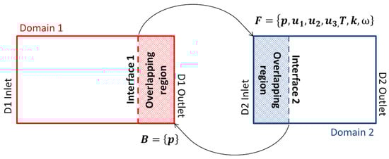
Figure 12.
Domain coupling with overlapping regions (adapted from [92]).
In the case of steady simulations, to reach a converged state where continuity was ensured between all the quantities in the two sub-domains required a certain number of cycles. Both solvers evolved through a series of stationary states, since time was not a variable of the computation. The coupling methodology for steady simulations was extensively described by Insinna et al. [24] and will be briefly described here. During the convergence process, each solver executed, separately from the other, a defined number of numerical iterations to evolve from one stationary state to the next one, thus converging to a solution that ensured consistency in space between the two sub-domains. It is worth underlining that the number of numerical iterations executed for each cycle could be different from one solver to the other, in order to consider that solvers could also be characterized by different convergence rates.
When unsteady simulations are executed, consistency must be ensured in both space and time, taking into account that solvers can advance in time with different time steps. If solvers run with the same time step (), the synchronization scheme is similar to the one used for steady simulations [24]. The only difference is that solvers do not advance anymore through stationary states but in physical time.
The case with is different. Considering, for example, a case with (see Figure 13), it must be considered that data exchange happens when solvers are at the same physical time. Therefore, the operations that must be performed are the following:

Figure 13.
Unsteady coupling methodology with different time steps [25].
- Solver 1 is initially at the state , which corresponds to the time , and, after receiving the feedback B from solver 2, starts to advance in time until reaching the state , which corresponds to the time ; solver 2 waits.
- Solver 1 passes F to solver 2. F contains time-averaged data, taken on a moving window, the amplitude of which can also be larger than the time interval .
- Solver 2 is initially at the state , which corresponds to the time and, after receiving the time-averaged F from solver 1, advances in time until reaching the state , which corresponds to the time ; solver 1 waits.
- Solver 2 passes B to solver 1 and the cycle restarts.
Some results obtained by using this methodology are reported in Figure 14, where instantaneous contours of turbulent kinetic energy in the wake region of the test case described by Sieverding et al. [133] are visible. Zarrillo [92] placed the overlapping region after the vane trailing edge and analyzed the formation of the von Karman vortex for a blunt trailing edge. Two different treatments of the outlet section of “Domain 1” are considered to verify the impact of Non-Reflecting Boundary Conditions (NRBC) [203] in the URANS simulation of coupled domains with overlapping regions. Although different levels of turbulence were individuated, the coupling methodology demonstrated its ability to correctly solve the unsteadiness at integral scale by allowing the vortex to continuously pass through the overlapping region.
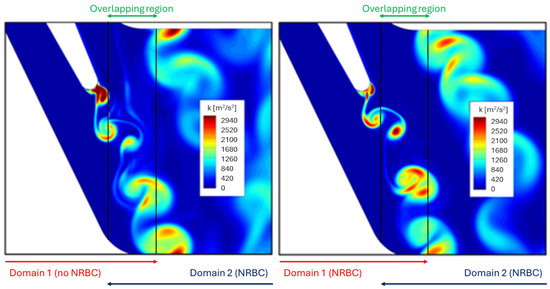
Figure 14.
Unsteady simulation of a blunt trailing edge test case with domain coupling and different treatments of Domain 1 outlet (adapted from [92]).
The scheme of synchronization here reported for unsteady domain coupling was originally proposed by Insinna [25] and was coherent with the so-called “staggered scheme” proposed by Collado Morata [149] for LES/RANS coupling. The reason why the case with was the most relevant for turbomachinery applications was that high-fidelity methods may be applied for the resolution of the combustor domain (namely “Domain 1”) and URANS might be used for the high-pressure turbine vane (“Domain 2”) [24]. In such cases, to obtain an adequate time resolution for the turbulent structures, the time step used for the combustor simulation should be lower than in the turbine domain where such methods are still hardly applicable. In those cases, a methodology for the proper treatment of turbulent variables at the interfaces (e.g., time-averaging of velocity fluctuations to create lossless boundary conditions for a RANS simulation) would be necessary. The turbulent kinetic energy exchanged between the domain through the F vector would be defined as , where should be calculated at runtime by considering flow fluctuations over a statistically representative time window. A simplified example of this turbulence treatment is reported in Figure 15, where Domain 1 was solved using SAS and Domain 2 was solved using URANS. As can be observed, the velocity fluctuations obtained in the first domain were transformed into boundary conditions for the second domain, where only integral-scale turbulence was solved.
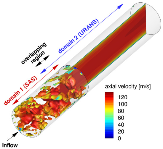
Figure 15.
Unsteady simulation of a turbulent pipe flow with domain coupling and different treatments for Domain 1 (SAS) and Domain 2 (URANS) [204].
The methodology detailed here should be considered as a baseline approach to the problem that could be modified depending on the specific case (e.g., compressor/combustor or combustor/turbine), solver (e.g., in-house or commercial), or approach (e.g., URANS or LES) that is used. Soli et al. [153] developed a methodology to efficiently simulate compressor/combustor coupling using URANS for the compressor and LES for the combustor, which was validated against experimental data. Results from that analysis were discussed in Section 3.1. Miki et al. [205] compared results obtained from the fully coupled and the decoupled simulations of the “Energy Efficient Engine” combustor [206] and turbine [207], and an integrated simulation using high-fidelity methods. Results obtained with the decoupled simulation were considered inaccurate, while fully coupled methods demonstrated their superior ability to capture flow physics, although only the integrated simulation individuated a low-pressure region downstream of the first-stage vane. The relevance of inlet conditions to accurately perform combustor/turbine simulation and the superior performance of an integrated approach were also demonstrated by [208]. A recent work by Tomasello et al. [82] confirmed that an integrated approach based on high-fidelity turbulence was recommendable for the accurate prediction of the heat transfer in cooled high-pressure vanes. Similar results were shown by Thomas et al. [209], where statistics of the unsteady heat load on an uncooled high-pressure vane were analyzed using LES, also underlining the importance of clocking position between the combustor and the vane. However, [210] underlined that a decoupled simulation showed acceptable results if compared with an integrated simulation when time-varying boundary conditions accounting for the effects of unsteadiness were used at the cooled vane inlet section. Tomasello et al. [210] also recommended the methodology proposed by Gründler et al. [211], which was based on the Proper Orthogonal Decomposition (POD) technique [212]. Gründler et al. [211] underlined that a high number of POD modes should be used not to filter the energy content.
3.3. Numerical Methods for Blade Row Interaction Analysis
From a physical point of view, the flow unsteadiness can be produced by potential interaction due to pitch-wise pressure distribution, by wake transport, and by secondary flows developed inside of the vanes. Furthermore, the presence of oblique shocks in transonic stages produces a complex system of shock reflections leading to boundary layer separation on the end-walls and blade surfaces (see also Section 2.9).
Several methods have been proposed for modelling vane/blade interaction. By now, the most used in industrial applications (e.g., blade profile design or optimization) is the steady approximation with the “mixing plane” approach. This method consists of a tangential average of the solution vector on the interface plane, then the interface boundary conditions are updated and the rows are solved separately. This kind of solution approximates a complete mixing of the flow from the upstream row, neglecting circumferential non-uniformities. Therefore, when using this method, the stagnation pressure at the interface plane is overestimated. Furthermore, steady calculations do not consider the nonlinear effects due to products of velocity field fluctuations. Hence, this approach can be used to estimate approximately the performance parameters but cannot provide the deep knowledge of the flow field inside of the turbine stage. For these reasons, the mixing-plane model is not going to be discussed here and the reader may refer to the papers by Giangiacomo et al. [213], Holmes [214], Denton [215], and Hanimann et al. [216] for more information.
To correctly evaluate the aerothermal field in turbine stages, several unsteady approaches have been proposed that can be enlisted as follows based on increasing complexity and simulation capability:
- Unsteady modelling using deterministic stresses.
- Quasi-unsteady simulations with unsteady boundary condition updating.
- Full unsteady simulations in time or frequency domains.
Advantages and limitations of the most relevant unsteady methods are discussed in Section 3.3.1, Section 3.3.2, Section 3.3.3, Section 3.3.4 and Section 3.3.5, where a baseline description of the models is reported. For more information about the underlying hypothesis of each model and their implementation in solvers for turbomachinery analysis, it is suggested to refer to the cited papers.
3.3.1. Deterministic Stresses
A “quasi-steady” approach to the unsteady modelling has been proposed by Adamczyk et al. [217]. Considering a single-stage configuration, the geometry of the neighboring blade rows, for which the blade count is not an integral multiple of the blade row of interest and which are stationary relative to this blade row, appeared smeared when using this method. For this case, the time-averaged flow field was not spatially periodic over the pitch of any given blade row. The spatial non-periodic flow field should be transformed into one that is periodic over the pitch of a given row. The resulting flow was called “average-passage” flow. With this approach, every row of a multistage configuration had its own averaged flow, while the rows were coupled with each other through a system of body forces, energy sources, and spatial correlations. This approach was similar to the Reynolds-averaging of Navier–Stokes equations. The steady part of the flow field was solved through the set of time-averaged equations, while the unsteady contributions were taken into account with time-averaged spatial correlations (“closures”) between the fluctuating flow variables.
To develop the model, the variables were decomposed into four parts: the axisymmetric (subscript ) component, the time-averaged absolute term as observed in a frame of reference fixed with the stationary row (subscript 1), the corresponding time-averaged term as observed from the moving blade row (subscript 2), and the unsteady contribution of both reference frames (subscript 3). Considering the velocity field, the decomposition could be written in a cylindrical reference frame, as in Equation (7).
In this decomposition, the axisymmetric value of the velocity v and the velocity field were steady because they were evaluated in the absolute frame of reference. A velocity component was also defined as in Equation (8).
The correlations which were present in the average passage momentum equations associated with the stationary blade row were obtained by performing the time-averaging of the product of the fluid density and a combination of and . Based on these considerations, the tensor is reported in Equation (9) (where the index is moved to superscript for sake of clarity).
In these equations, the subscripts take on the values from 1 to 3 and represent the axial z, the tangential , and the radial r components of the velocity field. These are the correlations between the average passage flow on the two rows. For example, for and , considering a low Mach number case and a constant value for the the density, is the relation between the density and the product between the axial and the tangential velocity of the fluctuating field. In a similar way, the total enthalpy H field was decomposed (Equation (10)) and the tensor was obtained (11).
For an inviscid, nearly irrotational flow, the magnitude of the component was less than the magnitude of v″ in most of the domain. Furthermore, in the regions where body forces and energy sources were finite, the correlation with v″ was higher than the one with . Then, it was assumed that the correlations associated with could be neglected in Equations (9) and (11), and finally, their value could be evaluated directly from the average passage solution. This means that the flow field through two rows was evaluated simultaneously and that an iterative procedure was used. In the first phase of the calculation, the body forces, the energy sources, and the correlations were not updated and an average flow field was evaluated considering their actual values and the boundary conditions. Once the convergence of this cycle was reached, all the correlations and the source terms were updated; this second cycle included the first one and decided when the convergence of the whole calculation was reached.
This method is continuously in development, trying to modify the way the deterministic stresses are obtained. Busby et al. [218] did not employ the average passage analysis and decomposed the velocity field u into a deterministic and a stochastic part. The deterministic part was then divided into a mean value and a deterministic fluctuation , as reported in Equation (12).
The stochastic part was due to turbulence and was modelled by Reynolds-averaging techniques. The mean value of the deterministic part was constant over all time scales and could be evaluated with the time-averaged solution. An analogous decomposition could be applied to the heat transfer. Busby et al. [218] considered an unsteady inviscid simulation and tried to evaluate by separating the deterministic fluctuations from the time-averaged solution. The obtained source terms were applied to a steady viscous calculation to obtain the unsteady flow field.
Even if Busby et al. [218] did not use the average passage equations, their method is ascribable to the deterministic stress group proposed by Adamczyk et al. [217]. The main difference between them was that in this case, the unsteady contribution in both the reference frames ( in Equation (9)) was considered inside of the value of the deterministic fluctuation term. Furthermore, using this method, Busby et al. [218] obtained a viscous solution with the following form of the tensor (Equation (13)):
One of the limitations of the method proposed by Busby et al. [218] was that they substitute a single unsteady viscous simulation with two faster but more complex simulations. In fact, to correctly evaluate the deterministic stress terms, it was necessary to reach convergence in the unsteady inviscid simulation. Then, a steady viscous simulation with modelled unsteadiness and turbulence was used, but even considering as perfectly converged the unsteady model, there were more equations to be solved than in a standard unsteady calculation. However, the results presented by the authors showed a good agreement between a real unsteady solution and the one obtained with this method, which could be considered for further developments.
In conclusion, the unsteady method based on the average passage equation system was interesting for its description of the unsteady interaction physics. Starting from the theory proposed by Adamczyk et al. [217], several unsteady methods were developed, especially in the field of the aero-acoustic interaction and the nonlinear harmonic methods [129,219,220,221].
3.3.2. Loosely Coupled Approach
Several methods have been developed to achieve viscous, time-accurate solutions for unsteady flows through isolated or aerodynamically coupled blade rows. In the latter case, two main categories of numerical procedures can be individuated. In the first category, both blade rows are modelled and the relative position between them is varied to simulate the motion. In the other category, the incoming wakes are specified at the inlet of an isolated blade row.
Dorney et al. [222] proposed to solve the vane/blade interaction with a Loosely Coupled Blade Row (LCBR) approach, which belonged to the second category. The unsteady boundary conditions were periodically updated at the interfaces to include the unsteady effects coming from the upstream and the downstream rows. The rows were then loosely coupled through the common unsteady boundary conditions. With this procedure, all of the blade passages could be solved simultaneously. Furthermore, the LCBR technique also has high computational efficiency because the underlying steady flow solutions needed to be solved in only one single passage of each blade row. In this numerical analysis, quasi-2D characteristic boundary conditions were solved implicitly along with the computational domain. After each time step, characteristic boundary conditions were explicitly applied at the inlet and exit boundaries to improve solution accuracy. This treatment, as it incorporates 2D unsteady boundary conditions based on the linearized Euler equations, assumed that the convection of the wakes and propagation of acoustic waves were inviscid phenomena. The proposed algorithm can be explained considering a simple 2D stage. First of all, two separated steady-state solutions for vane and blade were obtained, considering only one blade passage in each row. Then the steady solutions were copied to the appropriate number of blade passages to obtain the correct blade count ratio. After this passage, using the exit conditions of the vane row, the inlet condition of the blade row was obtained. For every conservative variable x, the local fluctuations of the steady solution were obtained considering the difference between the local value and the mean spatial value , as written in Equation (14).
These scaled perturbations were translated in the proper direction as a function of time, multiplied by the spatial mean of the blade inlet value and then added to the spatial mean of the blade inlet quantities. Finally, the value of a conservative variable at the blade inlet was written as in Equation (15):
The first term in Equation (15) was constant and represented the steady value at the blade inlet, while the second term represented the fluctuating contribution due to the interaction with the vane and was a function of time and position. Once the boundary conditions were updated, the unsteady effects in the blade could be computed. In a similar way, the unsteady information from the blade was imposed at the vane exit section, so the flow field in the vane could be solved considering unsteady boundary conditions at the exit plane. This procedure could be repeated many times for several global interaction steps until unsteady convergence was reached, while the time-averaged solution was used to update the fluctuations of the variables at the interface plane. The global convergence was reached when the differences between the perturbation values of two consecutive iterations were less than a specified value. This numerical method was tested considering several test cases and the obtained results was compared with both the available experimental data and with Fully Coupled Blade Row (FCBR) approach results. The LCBR method was ten times faster than the FCBR approach, maintaining a good accuracy. The main limits of this method were represented by geometries with small axial gaps and by the necessity of simulating more than one blade passage for every row. Furthermore, the definition of the unsteady fluctuation should be more accurate than the one presented. Nevertheless, this method seemed to be promising and several efforts have been made to eliminate the mentioned limitations and then improve the unsteady flow field evaluation.
3.3.3. Domain Scaling Approach
The Domain Scaling (DS) approach, also known as Reduced Count Ratio (RCR), proposed by Rai and Madavan [223] and Dawes [224], extended the sliding plane approach originally proposed by Rai [225,226] and Rai [227] to uneven blade counts. Considering a turbine stage with an unfavorable blade count (e.g., 43:64), using this approach, the number of the blades of one of the rows was changed to obtain computationally less expensive ratios (e.g., 1:2 or 2:3). The computational domain was then modified by using a quasi-homothetic reduction in the geometry in the axial and the tangential directions ( plane), while the radial extension was maintained. The Scaling Factor was a function of the real and the desired number of blades, as defined in Equation (16), where is the angle for a single blade and N is the number of blades.
A value of scaling factor near unity indicated a small modification of the geometry. This method allowed an FCBR approach to solve unsteadiness and seemed to represent an easy way to face the unsteady simulation, but must be used carefully. In fact, the variation of the blade number caused the modification of several blade characteristics, such as flow frequencies, throat area, and blade profile. An example of a modified blade geometry to move from a blade count of 43:64 to 42:63 at mid-span of the CT3 test cases analyzed by Salvadori et al. [125] and Ottanelli [123] is visible in Figure 16.
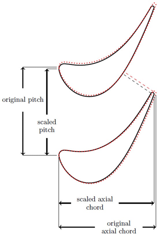
Figure 16.
Geometrical modifications generated by domain scaling at mid-span of the CT3 blade (red–dotted lines represent the unscaled geometry) [123].
Flow frequencies in a blade row are a function of the number of blades of the other row, as can be derived from Equations (17) and (18), where f is the deterministic frequency, is the rotational velocity in , and is the rotational velocity in rad/s.
A strong variation in the blade number could change its flow characteristics. In fact, the variation of the throat area of a vane could bring serious problems in transonic stages, while skewing the blade to maintain the throat area may introduce a variation in the pressure distribution on the blade. Arnone and Pacciani [228] analyzed all the major vane/blade combinations for the Nuovo Pignone PGT2 turbine to determine what was the acceptable pitch alteration to approximate the machine geometry without relevant impact on the mass flow rate and the flow physics. The authors concluded that if the adjustment in blade pitch was less than , no important deterioration was found in the results, including in the transonic regime.
Another example of the variation of the blade shape was associated with the MT1 test case by QinetiQ [33]. In this case, a scaling factor of (equivalent to a variation of ) was caused by the fact that the number of blades increased from 60 to 64, obtaining a blade count of 1:2. The vane (32 elements) was not modified to avoid modifications of the nominal mass flow rate. The value of the scaling factor was high and the variation of the throat section at mid-span was clearly visible, as well as the reduction in the axial chord of the blade and its solidity. Furthermore, a variation in the mean flow angles at the inlet and exit planes was found with respect to the real geometry. Examples of usage of the RCR technique in the same high-pressure turbine stage were reported by Salvadori et al. [229] and Simone et al. [30], whose results are extensively discussed in Section 2.5.
Recently, Wang et al. [230] developed an overset grid method for an efficient vane/blade coupling aimed at performing LES of high-pressure turbine stages. The MT1 test case was used to validate the methodology by applying the domain scaling technique to the vane, thus obtaining a 30:60 blade count with periodicity. Wang et al. [230] obtained results of comparable accuracy in terms of blade pressure distribution with respect to the ones shown by Salvadori et al. [229], but the data obtained by using frequency domain methods (see Ottanelli [123] and Section 3.3.5) were more accurate.
Even if the exact effect of the scaling cannot be quantified without a comparison either with an FCBR simulation or with experimental results, the RCR technique is widely used in industrial research thanks to its fast convergence rate and reduced computational cost. This could be justified considering that the approximation introduced by this method was acceptable if the scaling factor was near unity [228]. Considering the CT3 test case [117,118,123,125], passing from 43:64 to 42:63 (and then 2:3; see Figure 16), a scaling factor of was obtained for the vane and for the blade. Furthermore, the blade count changed from to , which was a variation of . In such cases, the deterministic part of the velocity fluctuation caused by the geometrical properties remained unaltered, as confirmed by the comparison between experimental and RCR results shown in Figure 17.
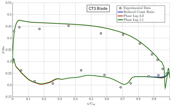
Figure 17.
Time-averaged non-dimensional static pressure distribution at CT3 blade mid-span calculated using 2D CFD with both domain scaling and phase lag techniques (adapted from [123]).
A modified approach to domain scaling is the profile transformation method proposed by [231] and Connell et al. [232]. In this case, the geometrical characteristics of vanes and blades were not modified but the interface flow field was scaled to match the exact angle of opening of each row. This approach allowed for simulating the full annulus with a single-passage simulation, but suffered from the same limitations that characterized the RCR approach. In fact, for unfavorable blade counts in the scaling procedure greatly modified the flow field.
Concluding, the RCR approach is a powerful method to simulate uneven blade counts. However, it is characterized by a serious drawback which makes it less useful for high scaling factors. The time lag approach as well as frequency domain and harmonic methods, which are able to correctly simulate a complete annulus by modelling single passages (see Section 3.3.5 for more details), are the most promising solutions to the uneven blade count simulation problem.
3.3.4. Time Lag or Time Inclining
Giles [233] and Giles [234] developed a method for treating unsteady flows for single and multiple perturbations without any geometrical modification. Considering a blade row, with a wake modelled at the inlet as a boundary condition, if the wake had the same pitch of the blade, the periodic boundary condition could be directly imposed. Instead of a wake model, a vane could be coupled with the blade row. Again, if the pitches were equal to each other, the main problem was the coupling of the computational grids on the hanging section. Considering the same grid spacing along the interface on both sides, the authors proposed to connect the two rows using a series of sharing nodes [233,234]. As time advanced, the blade moved tangentially and the spatial periodicity was used to move the blade grid accordingly, thus obtaining the correct periodicity in time. The use of this approach imposed the conversion of all the flow variables in the chosen frame of reference. A detailed description of the proposed algorithm is available in [235].
If the vane number was not equal to the number of blades, the spatial periodicity in the pitch-wise direction could not be treated as previously detailed. This remark remained valid when considering a single row with unsteady boundary conditions that were characterized by a different periodicity of the perturbation with respect to the row.
Considering two different instants in a turbine stage for a generic blade count as reported in Figure 18, blade number 1 is clocked with respect to vane number 1 at time t in the same geometrical position of blade number 2 with respect to vane number 2 at time . The time lag that occurs between these two positions is a function of the pitches P and of the tangential velocity , as shown in Equation (19):
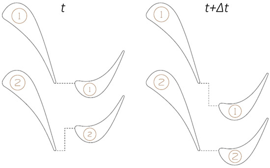
Figure 18.
Relative position between vane and blade for a generic blade count (adapted from [123]).
The state of the flow on the lower periodic surface () is equal to the one on the upper surface but considered at a different timing (). Erdos et al. [236] proposed a method to numerically evaluate the flow field and to implement the lagged periodic boundary conditions. Dummy nodes were used along a periodic line to store the actual values obtained by the knowledge of the values on the other periodic lines but at different time steps. The periodicity was imposed by using the equivalences reported in Equation (19) for both vane and blade rows on the upper and lower boundary.
Even if this method is explained in Section 3.3.5, its main limits can be already summarized to better understand the differences between the approach proposed by Giles [235] and the one by Erdos et al. [236]. In the latter, to update the values in the dummy nodes, the solution on the periodic lines was stored over a complete periodicity, thus causing a large expense in terms of computational costs. Furthermore, the frequencies of the flow variables that were updated were a function of the blade number, and then only the deterministic unsteadiness could be evaluated. Since several unsteady phenomena are not perfectly governed by the vane or the blade frequencies, a full unsteady convergence could not be reached. For example, considering the vortex shedding phenomenon, the use of the deterministic unsteadiness forced the solver to match a synchronous shedding in which each blade shed vortices characterized by the same sign at the same time step. However, even if a temporal synchronization could be possible, the sign for two adjacent blades should be opposite each other. However, within these limitations, the main part of the unsteady phenomena could be evaluated and the frequency corresponding to a specific phenomenon, if known, could be explicitly imposed as a boundary condition, as explained in Section 3.3.5.
On the contrary, Giles [235] proposed a space–time transformation method to implement the phase-shifted periodic condition and overcome the limitations of the method by Erdos et al. [236]. In this case, the time plane in the computational domain was inclined along the pitch-wise direction according to a given inter-blade phase angle. The phase-shifted periodic condition could then be directly applied by matching the flow variables at the periodic boundaries. Therefore, no extra storage was required and the convergence rate was faster if compared with the method by Erdos et al. [236] since the numerical procedure was less influenced by the initial guess. However, the time inclination angles (and therefore the allowed inter-blade phase angles) were restricted by the velocity of the travelling wave in the tangential direction at the vane/blade interface, which were taken into account by calculating the Mach number in the tangential direction , the rotational Mach number , and the ratio . A complete description of both the derivation of these constraints and the necessary modifications to be performed on the Navier–Stokes set of equations to solve vane/blade interaction with different pitches using the time inclining method is available in the papers by Giles [233,235] and Giles [234].
The method by Giles [235] was fast, computationally less expensive than most of the others, and had no limitations in the temporal periodicity. However, data processing was complex since the time-resolved data were reconstructed along the computational plane once convergence was reached. Second, the modification of the governing equations into a new time/space coordinate system [235] was a complex operation to be carried out on an existing solver.
3.3.5. Direct Storage and Shape Correction Methods
Methods based on the “phase lag” between the periodic boundaries do not require geometrical approximations and use the correlation between the spatial and the temporal periodicity to update the solution in single- and multi-row simulations. The first study on this approach was proposed by Erdos et al. [236], who presented the “Direct Storage” technique. Then, Koya and Kotake [237] extended the method to viscous stages, He [238] developed the “Shape Correction” method, and He [100] and Li and He [239] completed the development of methods based on phase-lagged boundary conditions through the “Generalized Shape Correction”, which allowed for considering multiple perturbations.
In detail, the “Direct Storage” method introduced by Erdos et al. [236] was firstly applied to a 2D stage where both vane and blade were modelled with a single passage (e.g., a single vane and a single blade were modelled in each row). The effects of heat transfer and viscosity were initially neglected and the Euler equations were solved. The main objective was to obtain an unsteady periodic solution of the flow field inside of the vanes. Erdos et al. [236] observed that the spatial periodicity was linked to the temporal evolution of the flow field. The method proposed by Erdos et al. [236] was based on the storage of flow variables at the periodic boundaries for one period in time. The stored parameters and the current solution corrected each other using a phase-shifted periodicity. That theory was explained in [236] by considering two examples characterized by a 3:3 blade count and a 3:4 blade count. The main disadvantages of the “Direct Storage” method were both a large amount of computer storage and a limited blade ratio that could be handled with this methodology. The latter was associated with the necessity to store a sufficient amount of data along the interfaces to provide information for a maximum period corresponding to the blade passing frequency of the row with the smaller number of blades.
To deal with the phase-shifted periodicity, He [238] proposed a method called “Shape Correction” (also know as “Phase-Lagged Boundary Conditions”). In this method, instead of directly storing the flow parameters, only the Fourier coefficients of flow variables at the periodic boundaries and at the interfaces were stored so that the memory usage was reduced. The stored temporal shape of flow variables was then used to correct the current solution at the periodic boundaries. However, that method could only be used to deal with unsteady flows with a single perturbation. In practice, several unsteady perturbations with their own phase-shifted periodicity coexist in a turbine stage. To overcome that limit, a generalized version of the “Shape Correction” method that allowed a single passage solution for unsteady turbomachinery flows with multiple perturbations was proposed by He [100]. The main hypothesis of the new method was that all the unsteady perturbations satisfied a temporal and spatial periodicity characterized by a specific wavelength and a constant travelling velocity along the circumferential direction.
The “Phase Lag” method for multiple perturbations allowed for using a single passage periodicity in the multi-row simulations since the solution was updated using the correlation between the spatial and the temporal fluctuations of the variables. The unsteady solution was decomposed by the Fourier series coefficients, which were used to update the periodic and interface boundaries [100,238].
Considering Figure 19, the method for the reconstruction of the correct values on the periodic faces and at the interfaces is based on the fact that for a single passage simulation at the time , the upper periodic is coupled with the lower periodic at time , where P is the pitch value and is the tangential velocity of the row. Similarly, the lower periodic is coupled with the upper periodic at time . This allowed for calculating the correct flow variables at the interface and at the periodic boundaries using Equation (20), where U is the vector of the conservative variables, is the time-averaged solution, represents the unsteady part of the flow field with the spatial and temporal periodicity of the perturbation, and is the total number of perturbations used to calculate the unsteady flow field.
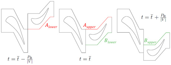
Figure 19.
Phase-shifted periodicity to be applied to single-passage simulations of turbine stages (adapted from [123]).
The fluctuating part of the solution can be approximated using the Fourier series in time as in Equation (21), where is the number of harmonics, and are the Fourier series coefficients, is the pulsation associated to the perturbation, and is the phase shift.
Care should be taken while choosing the number of perturbations . Due to moving boundaries or blade flutter, the geometrically defined perturbations were usually determined by known parameters such as blade number and rotational speed and will then be considered as “fundamental” perturbations. In the case of multi-row simulations, neglecting the flutter effects, the main frequencies were defined by the blade number of the rows and the rotational speed. These fundamental frequencies were responsible for the deterministic stresses already described in [217]. If the nonlinear interactions between the fundamental perturbations are not strong, can be set equal to the number of the deterministic frequencies. The interaction between the chosen perturbations and the steady flow manifests in the amplitude and the phase of the corresponding part. Considering the spatial and temporal periodicity assumption, the value of in Equation (21) can be written as in , where is the circumferential distance from a reference point, while is the circumferential travelling speed of the perturbation at the radius r.
The same procedure could be used to update the boundary values along the interfaces between the domains in the case of multi-row simulation. Considering a turbine stage, the flow field on both the interfaces was decomposed in its Fourier series coefficients obtaining the “shape” of the solution on the interfaces using Equation (21). When the boundaries were updated, the flow field on the vane and blade interfaces updated one another, taking into account the relative position (starting from a known initial state) and the timing. For every time step, the correspondences between the nodes on each interface were a matter of geometrical parameters and of the rotational velocity only (e.g., ). For instance, the solution on a face of the rotational row can be recovered with the formula in Equation (20) imposing (because the phase angle could be taken into account during the preliminary processing of the interfaces) and using the actual value of the time. The obtained result will be used to update the solution on the corresponding face of the vane row. Since an exact correspondence between the nodes was not possible, an interpolation procedure was necessary.
To run the computation, a time-marching procedure can be started with an assumed shape of the boundary conditions on the interface and periodic faces. Then, the flow field and the stored shape could be used to update each other using the phase-shifted periodicity, until convergence was reached. The core of this method was the implementation of the updating procedure for the Fourier series coefficients and . In the case of a single perturbation, the Fourier coefficients could be updated every period using Equations (22) and (23):
In Equations (22) and (23), is the number of time steps in one period. In the case of multiple perturbations, the coefficients could be updated only when all the frequencies of the perturbations caused a beat after a certain number of periods. In practice, the beating period could be longer than the single perturbation period and the time-marching solution could be slowed down. To obtain a faster convergence, the coefficients could be updated every period of the corresponding perturbation using the approximate form of the solution vector U defined in Equations (24)–(26).
and could be updated once a period for the corresponding perturbation if the value of calculated by Equation (24) was used. The value of was representative of the part of the solution that was not affected by the perturbation. This procedure introduced a source of error since the value of was evaluated approximately, but it allowed for a faster convergence rate. Furthermore, the expressions in Equations (25) and (26) provided a solution of the same order of accuracy of Equations (22) and (23) for a single perturbation, and the final result was not affected by the use of Equation (24).
This method has been validated on several test cases and demonstrated faster convergence if compared with the “Direct Storage” method as well as a good accuracy of the solution. An example of successful implementation of the phase-lagged boundary conditions is reported in Figure 17, where the blade load at mid-span of the CT3 test case [118] obtained using a domain scaling approach is compared with results obtained by Ottanelli [123] using a in-house solver developed by Salvadori et al. [125]. All the calculations were performed using the same computational grid and a scaled 2D geometry, thus allowing for a meaningful comparison. As can be observed, negligible differences can be found between a full unsteady approach (“Reduced Count Ratio”) and a Fourier-based simulation on a 2:3 domain (“Phase Lag 2–3”) and a single passage simulation (“Phase Lag 1–1”), thus demonstrating the accuracy of the proposed unsteady method. More information about the implementation procedures of phase-lagged boundary conditions can be found in [100,122,123,124,125,129,238,239,240,241]. Also, modified versions of this method were proposed by Issa and Sadri [242] and Gerolymos et al. [39].
Among the Fourier-based methods for the simulation of nonlinear unsteady flows in turbomachinery, the harmonic balance technique developed by [132,219,220] deserves to be mentioned thanks to its computational efficiency and its ease of implementation. The harmonic balance method was based on the assumption that turbomachinery flows were usually periodic in time thanks to the deterministic nature of integral-scale fluctuations, which were related to rotational speed and blade count. Therefore, unsteady variables can be represented by a Fourier series in time with spatially varying coefficients by extending the procedure reported from Equations (20)–(26) to all the computational nodes. This method was particularly well-suited for the computation of the aerodynamic forces that produce flutter in turbomachinery [219], but could be also used for multistage coupling [220]. More information about the harmonic balance technique and its implementation can be found in the cited references.
4. Conclusions
In the present paper, an overview of unsteady flow characteristics and component interaction in gas turbines is presented. Several topics have been discussed, with special interest on the redistribution of non-uniformities from the combustor in high-pressure turbine stages, on the description of the existing test rigs for compressor/combustor and combustor/turbine interaction analysis, and on the description of the most relevant numerical methodologies for component interaction and vane/blade interaction. The following general conclusions can be drawn:
- The impact of stagnation pressure non-uniformities on the turbine performance is negligible, with the maximum non-uniformity being lower than . However, non-negligible effects were found when an increase in stagnation pressure was found close to the end-walls because it affected the development of secondary flows.
- The stagnation line on high-pressure vanes is modified by the presence of a residual swirl from the combustor, especially in lean-burn configurations. In fact, fluctuations of in the incidence were found close to the end-walls, thus causing the modification of the stagnation point location up to axial chords. The radial variation of incidence also generates a radial distribution of loading.
- Stagnation temperature circumferential non-uniformities are responsible for the migration of hot flow towards the high-pressure blade suction side due to the “positive jet” effect that interacts with the passage vortex. An increase in Nusselt number value by was observed on the blade pressure side at mid-span. Moreover, a reduction in the residual blade life up to ≈ was associated with an increase of ≈+40 K in metal temperature. The passage vortex is also responsible for the migration of the hot flow towards the tip clearance and for its interaction with the tip leakage vortex.
- Coolant flow distribution is driven both by the non-uniform cooling hole outlet pressure distribution generated by residual swirls and by the modified development of secondary flows. Variations in coolant mass flow rate of were found in a linear case with a strong residual inlet swirl profile. Moreover, the usage of a mean driving temperature value for heat transfer calculations may provide inaccurate results during the design process.
- Existing test rigs for compressor/combustor and combustor/turbine interaction analysis allowed for accurately studying the most relevant phenomena occurring in gas turbines in engine-relevant conditions. Experimental results were also of great relevance for the solver verification, calculation validation, and uncertainty quantification.
- Even though non-uniform air feeding to burners was experimentally found, compressor/combustor interaction generated negligible effects when compared with combustor/turbine interaction (at least for the investigated configurations). However, it was possible to individuate the high-pressure compressor rotor passing frequency in the primary zone of the combustor through a frequency domain analysis, thus hinting at an interaction with combustion instabilities.
- Either fully coupled or integrated simulations were necessary to correctly analyze the aerothermal characteristics of cooled high-pressure turbine stages due to the impact associated with the unsteadiness and the turbulence on both loading and heat transfer. Concerning the latter, scale-resolving methods were necessary to correctly simulate heat transfer coefficients on cooled vane surfaces, with SBES being the most promising approach thanks to its reduced computational cost with respect to LES. Such approaches were also necessary to take into account the “net circulation” phenomenon, which was responsible for the circumferential movement of the residual swirl.
- Concerning vane/blade interaction, frequency domain methods proved to be accurate methods for the analysis of a wide range of phenomena and showed a remarkable convergence rate. However, all the methods presented here were sufficiently accurate for the study of turbine stages and the selection of the most suitable one mostly depended on the problem that was investigated and on the available computational resources.
Author Contributions
Writing—original draft preparation, S.S. and M.I.; writing—review and editing, S.S., M.I. and F.M.; supervision, S.S. and F.M. All authors have read and agreed to the published version of the manuscript.
Funding
This research received no external funding.
Institutional Review Board Statement
Not applicable.
Informed Consent Statement
Not applicable.
Data Availability Statement
Data is contained within the article.
Acknowledgments
The authors are grateful to Luca Ottanelli and Marilena Zarrillo for the support provided in the preparation of the manuscript.
Conflicts of Interest
The authors declare no conflicts of interest.
Nomenclature
The following nomenclature is used in this manuscript:
| a | sound speed [m/s] |
| A | amplitude of an oscillation [m] |
| b | bi-normal direction [−] |
| B | vector of variables |
| c | absolute velocity [m/s] |
| C | chord |
| d | dump gap [m] |
| f | frequency [Hz] |
| F | force [N/m2], vector of variables |
| axial flux of momentum [(kg · m)/s2] | |
| axial flux of momentum [(kg · m2)/s2] | |
| h | enthalpy [kJ/(kg · K)], pre-diffuser exit radius [m] |
| H | total enthalpy [kJ/(kg · K)] |
| k | kinetic energy [m2/s2], turbulent kinetic energy [m2/s2] |
| n | normal direction [−] |
| N | number of airfoils, number |
| p | pressure [Pa] |
| P | pressure [Pa], pitch [m] |
| Q | tensor |
| r | radius [m] |
| R | radius [m], tensor, Fourier series residual [m/s] |
| s | stream-wise direction [−] |
| S | blade pitch [m], entropy [kJ/kg] |
| swirl number [−] | |
| t | time [s] |
| T | temperature [K], time period [s] |
| turbulence level [−] | |
| u | velocity [m/s], tangential velocity [m/s], velocity component [m/s] |
| U | velocity [m/s] |
| v | velocity [m/s] |
| V | tangential velocity [m/s] |
| w | relative velocity [m/s] |
| W | work [J] |
| x | axial gap [m], displacement [m] |
| y | Cartesian y-direction value [m] |
| Subscripts and Superscripts | |
| average value, deterministic value | |
| double average, deterministic value | |
| steady solution | |
| ′ | fluctuating value, stochastic value |
| ″ | double fluctuating value, stochastic value |
| 0 | stagnation condition, initial time step, averaged value |
| stationary reference frame | |
| moving reference frame | |
| both stationary and moving reference frame | |
| A | Fourier series coefficient [m/s] |
| axial | |
| B | vibrational, Fourier series coefficient [m/s] |
| turbine blade | |
| turbine casing | |
| combustion chamber | |
| fluid–blade | |
| harmonics | |
| turbine hub | |
| hot spot | |
| i | counter |
| j | counter |
| L | laminar |
| lower periodic | |
| maximum value | |
| mean value | |
| minimum value | |
| mass-weighted averaged | |
| n | counter |
| modified value | |
| nominal condition | |
| outlet section | |
| perturbation | |
| R | rotor |
| actual value | |
| slip flow | |
| s | stall condition |
| stall condition | |
| swirl | |
| T | turbulent |
| time averaged | |
| tangential | |
| total | |
| time step | |
| upper periodic | |
| turbine vane | |
| turbine wake | |
| x | axial direction |
| z | axial direction |
| Greek Letters | |
| dissipation rate [m2/s3] | |
| density [kg/m3] | |
| phase shift | |
| PI Greek | |
| phase shift | |
| tangential | |
| vane angle [deg] | |
| vorticity [1/s], specific dissipation rate [1/s], pulsation [1/s], rotational speed [rad/s] | |
| rotational speed [RPM] | |
| Abbreviations | |
| CFD | Computational Fluid Dynamics |
| CHT | Conjugate Heat Transfer |
| DES | Detached Eddy Simulation |
| DLN | Dry Low |
| DS | Domain Scaling |
| HSV | Horseshoe Vortex |
| HWA | Hot Wire Anemometer |
| ITD | Inlet Temperature Distortion |
| LES | Large-Eddy Simulation |
| NRBC | Non-Reflecting Boundary Conditions |
| OGV | Outlet Guide Vane |
| OTDF | Overall Temperature Distortion Factor |
| PIV | Particle Image Velocimetry |
| POD | Proper Orthogonal Decomposition |
| PV | Passage Vortex |
| PVC | Precessing Vortex Core |
| PS | Pressure Side |
| PSP | Pressure-Sensitive Paint |
| RTDF | Radial Temperature Distortion Factor |
| RANS | Reynolds-Averaged Navier–Stokes |
| RQL | Rich–Quench–Lean |
| RSM | Reynolds-Stress Model |
| SAS | Scale-Adaptive Simulation |
| SBES | Stress-Blended Eddy Simulation |
| SF | Scaling Factor |
| SS | Suction Side |
| SSG | Speziale–Sarkar–Gatski |
| SST | Shear Stress Transport |
| TLV | Tip Leakage Vortex |
| URANS | Unsteady Reynolds-Averaged Navier–Stokes |
References
- Lakshminarayana, B. Fluid Dynamics and Heat Transfer of Turbomachinery; Wiley: Hoboken, NJ, USA, 1995. [Google Scholar] [CrossRef]
- Rolls-Royce. The Jet Engine; John Wiley & Sons: Hoboken, NJ, USA, 2015. [Google Scholar]
- Paniagua, G. Investigation of the Steady and Unsteady Performance of a Transonic hp Turbine. Ph.D. Thesis, Université Libre de Bruxelles, Bruxelles, Belgium, 2002. [Google Scholar]
- Montomoli, F.; Carnevale, M.; D’Ammaro, A.; Massini, M.; Salvadori, S. Uncertainty Quantification in Computational Fluid Dynamics and Aircraft Engines; Springer International Publishing: Berlin/Heidelberg, Germany, 2015. [Google Scholar] [CrossRef]
- Parker, R. Paper 1: Relation between Blade Row Spacing and Potential Flow Interaction Effects in Turbomachines. Proc. Inst. Mech. Eng. Conf. Proc. 1969, 184, 1–8. [Google Scholar] [CrossRef]
- Greitzer, E. Introduction to unsteady flow in turbomachines. Unsteady Flow Turbomach. 1984, 1–62. [Google Scholar]
- Sieverding, C.H. Recent Progress in the Understanding of Basic Aspects of Secondary Flows in Turbine Blade Passages. J. Eng. Gas Turbines Power 1985, 107, 248–257. [Google Scholar] [CrossRef]
- Langston, L. Secondary Flows in Axial Turbines—A Review. Ann. N. Y. Acad. Sci. 2006, 934, 11–26. [Google Scholar] [CrossRef]
- Salvadori, S.; Montomoli, F.; Martelli, F.; Adami, P.; Chana, K.S.; Castillon, L. Aerothermal Study of the Unsteady Flow Field in a Transonic Gas Turbine With Inlet Temperature Distortions. J. Turbomach. 2011, 133, 031030. [Google Scholar] [CrossRef]
- Langston, L.S. Crossflows in a Turbine Cascade Passage. J. Eng. Power 1980, 102, 866–874. [Google Scholar] [CrossRef]
- Délery, J.M. Robert Legendre and Henri Werlé: Toward the Elucidation of Three-Dimensional Separation. Annu. Rev. Fluid Mech. 2001, 33, 129–154. [Google Scholar] [CrossRef]
- Lakshminarayana, B.; Horlock, J.H. Generalized expressions for secondary vorticity using intrinsic co-ordinates. J. Fluid Mech. 1973, 59, 97–115. [Google Scholar] [CrossRef]
- Denton, J.D. Loss Mechanisms in Turbomachines; American Society of Mechanical Engineers: New York, NY, USA, 1993; Volume 78897. [Google Scholar] [CrossRef]
- Kerrebrock, J.L.; Mikolajczak, A.A. Intra-Stator Transport of Rotor Wakes and Its Effect on Compressor Performance. J. Eng. Power 1970, 92, 359–368. [Google Scholar] [CrossRef]
- Dorney, D.; Davis, R.; Edwards, D.; Madavan, N. Unsteady analysis of hot streak migration in a turbine stage. J. Propuls. Power 1990, 8, 520–529. [Google Scholar] [CrossRef]
- Pullan, G. Secondary Flows and Loss Caused by Blade Row Interaction in a Turbine Stage. J. Turbomach. 2006, 128, 484–491. [Google Scholar] [CrossRef]
- Payne, S.; Ainsworth, R.; Miller, R.; Moss, R.; Harvey, N. Unsteady loss in a high pressure turbine stage. Int. J. Heat Fluid Flow 2003, 24, 698–708. [Google Scholar] [CrossRef]
- Qureshi, I.; Beretta, A.; Povey, T. Effect of Simulated Combustor Temperature Nonuniformity on HP Vane and End Wall Heat Transfer: An Experimental and Computational Investigation. J. Eng. Gas Turbines Power 2011, 133, 031901. [Google Scholar] [CrossRef]
- Shahpar, S.; Caloni, S. Aerodynamic Optimization of High-Pressure Turbines for Lean-Burn Combustion System. J. Eng. Gas Turbines Power 2013, 135, 055001. [Google Scholar] [CrossRef]
- Hall, B.F.; Chana, K.S.; Povey, T. Design of a Non-Reacting Combustor Simulator with Swirl and Temperature Distortion with Experimental Validation. In Proceedings of the ASME Turbo Expo 2013: Turbine Technical Conference and Exposition, San Antonio, TX, USA, 3–7 June 2013. ASME Paper No. GT2013-95499. [Google Scholar] [CrossRef]
- Barringer, M.D.; Thole, K.A.; Polanka, M.D. An Experimental Study of Combustor Exit Profile Shapes on Endwall Heat Transfer in High Pressure Turbine Vanes. J. Turbomach. 2009, 131, 021009. [Google Scholar] [CrossRef]
- Barringer, M.D.; Thole, K.A.; Polanka, M.D.; Clark, J.P.; Koch, P.J. Migration of Combustor Exit Profiles Through High Pressure Turbine Vanes. J. Turbomach. 2009, 131, 021010. [Google Scholar] [CrossRef]
- Insinna, M.; Salvadori, S.; Martelli, F.; Adami, P.; Vazquez, R. Aero-Thermal Analysis of Combustor/Turbine Interaction in Aero-Engines: The Challenge of Today. Available online: https://aerospace-europe.eu/case-studies/aero-thermal-analysis-of-combustorturbine-interaction-in-aero-engines-the-challenge-of-today/abstract/ (accessed on 25 January 2024).
- Insinna, M.; Salvadori, S.; Martelli, F. Simulation of Combustor/NGV Interaction Using Coupled RANS Solvers: Validation and Application to a Realistic Test Case. In Proceedings of the ASME Turbo Expo 2014: Turbine Technical Conference and Exposition, Düsseldorf, Germany, 16–20 June 2014; Volume 45622, p. V02CT38A010. [Google Scholar] [CrossRef]
- Insinna, M. Investigation of the Aero-Thermal Aspects of Combustor/Turbine Interaction in Gas Turbines. Ph.D. Thesis, Department of Industrial Engineering, University of Florence, Florence, Italy, 2014. [Google Scholar]
- Cha, C.M.; Hong, S.; Ireland, P.T.; Denman, P.; Savarianandam, V. Experimental and Numerical Investigation of Combustor–Turbine Interaction Using an Isothermal, Nonreacting Tracer. J. Eng. Gas Turbines Power 2012, 134, 081501. [Google Scholar] [CrossRef]
- You, D.; Ham, F.; Moin, P. Large-Eddy Simulation Analysis of Turbulent Combustion in a Gas Turbine Engine Combustor; Annual Research Briefs 2008; Center for Turbulence Research: Stanford, CA, USA, 2008; pp. 219–230. [Google Scholar]
- Butler, T.; Sharma, O.; Joslyn, H.; Dring, R. Redistribution of an inlet temperature distortion in an axial flow turbine stage. J. Propuls. Power 1986, 5, 64–71. [Google Scholar] [CrossRef]
- Munk, M.; Prim, R. On the Multiplicity of Steady Gas Flows Having the Same Streamline Pattern. Proc. Natl. Acad. Sci. USA 1947, 33, 137–141. [Google Scholar] [CrossRef]
- Simone, S.; Montomoli, F.; Martelli, F.; Chana, K.S.; Qureshi, I.; Povey, T. Analysis on the Effect of a Nonuniform Inlet Profile on Heat Transfer and Fluid Flow in Turbine Stages. J. Turbomach. 2012, 134, 011012. [Google Scholar] [CrossRef]
- Rai, M.; Dring, R. Navier–Stokes analyses of the redistribution of inlet temperature distortions in a turbine. J. Propuls. Power 1987, 6, 276–282. [Google Scholar] [CrossRef]
- Povey, T.; Chana, K.; Jones, T.V.; Hurrion, J. The Effect of Hot-Streaks on HP Vane Surface and Endwall Heat Transfer: An Experimental and Numerical Study. J. Turbomach. 2005, 129, 1483–1497. [Google Scholar] [CrossRef]
- Adami, P.; Salvadori, S.; Chana, K.S. Unsteady Heat Transfer Topics in Gas Turbine Stages Simulations. In Proceedings of the ASME Turbo Expo 2006: Power for Land, Sea, and Air, Barcelona, Spain, 8–11 May 2006; Volume 6, pp. 1733–1744. [Google Scholar] [CrossRef]
- Hilditch, M.A.; Fowler, A.; Jones, T.V.; Chana, K.S.; Oldfield, M.L.G.; Ainsworth, R.W.; Hogg, S.I.; Anderson, S.J.; Smith, G.C. Installation of a Turbine Stage in the Pyestock Isentropic Light Piston Facility. In Proceedings of the ASME 1994 International Gas Turbine and Aeroengine Congress and Exposition, Hague, The Netherlands, 13–16 June 1994. [Google Scholar] [CrossRef]
- Chana, K.; Mole, A. Summary of Cooled NGV and Uncooled Rotor Measurements from the MT1 Single Stage High Pressure Turbine in the DERA Isentropic Light Piston Facility; Brite-EuRam Turbine Aero-Thermal External Flow project (BRPR-CT97-0519); DERA: London, UK, 2002. [Google Scholar]
- Chana, K.S.; Jones, T.V. An Investigation on Turbine Tip and Shroud Heat Transfer. J. Turbomach. 2003, 125, 513–520. [Google Scholar] [CrossRef]
- Povey, T.; Qureshi, I. Developements in Hot-Streak Simulators for Turbine Testing. J. Turbomach. 2009, 131, 031009. [Google Scholar] [CrossRef]
- Chana, K.S.; Hurrion, J.R.; Jones, T.V. The Design, Development and Testing of a Non-Uniform Inlet Temperature Generator for the QinetiQ Transient Turbine Research Facility. In Proceedings of the ASME Turbo Expo 2003, Collocated with the 2003 International Joint Power Generation Conference, Atlanta, GA, USA, 16–19 June 2003; Volume 36894, pp. 273–280. [Google Scholar] [CrossRef]
- Gerolymos, G.A.; Michon, G.J.; Neubauer, J. Analysis and Application of Chorochronic Periodicity in Turbomachinery Rotor/Stator Interaction Computations. J. Propuls. Power 2002, 18, 1139–1152. [Google Scholar] [CrossRef]
- Castillon, L. Evaluation of a multiple frequency phase lagged method for unsteady numerical simulations of multistage turbomachinery. In Proceedings of the 28th International Congress of the Aeronautical Sciences, Brisbane, Australia, 23–28 September 2012. [Google Scholar]
- Thorpe, S.J.; Miller, R.J.; Yoshino, S.; Ainsworth, R.W.; Harvey, N.W. The Effect of Work Processes on the Casing Heat Transfer of a Transonic Turbine. J. Turbomach. 2007, 129, 84–91. [Google Scholar] [CrossRef]
- Roback, R.J.; Dring, R.P. Hot Streaks and Phantom Cooling in a Turbine Rotor Passage: Part 1—Separate Effects. J. Turbomach. 1993, 115, 657–666. [Google Scholar] [CrossRef]
- Roback, R.J.; Dring, R.P. Hot Streaks and Phantom Cooling in a Turbine Rotor Passage: Part 2—Combined Effects and Analytical Modeling. J. Turbomach. 1993, 115, 667–674. [Google Scholar] [CrossRef]
- Dorney, D.J.; Gundy-Burlet, K. Hot-streak clocking effects in a 1-1/2 stage turbine. J. Propuls. Power 1996, 12, 619–620. [Google Scholar] [CrossRef]
- Gundy-Burlet, K.L.; Dorney, D.J. Influence of 3D Hot Streaks on Turbine Heat Transfer. In Proceedings of the ASME 1997 International Gas Turbine and Aeroengine Congress and Exhibition, Orlando, FL, USA, 2–5 June 1997; Volume 14, pp. 123–132. [Google Scholar] [CrossRef]
- Shang, T.; Epstein, A.H. Analysis of Hot Streak Effects on Turbine Rotor Heat Load. J. Turbomach. 1997, 119, 544–553. [Google Scholar] [CrossRef]
- He, L.; Menshikova, V.; Haller, B.R. Influence of Hot Streak Circumferential Length-Scale in Transonic Turbine Stage. In Proceedings of the ASME Turbo Expo 2004: Power for Land, Sea, and Air, Vienna, Austria, 14–17 June 2004; ASME Paper No. GT2004-53370. pp. 1117–1126. [Google Scholar]
- Saxer, A.P.; Felici, H.M. Numerical Analysis of Three-Dimensional Unsteady Hot Streak Migration and Shock Interaction in a Turbine Stage. J. Turbomach. 1996, 118, 268–277. [Google Scholar] [CrossRef]
- Dorney, D.J.; Gundy-Buriet, K.L. Effects of Hot Streak Shape on Rotor Heating in a High-Subsonic Single-Stage Turbine. Int. J. Turbo Jet Engines 2001, 18, 15–30. [Google Scholar] [CrossRef]
- Dorney, D.J.; Sondak, D.L. Effects of Tip Clearance on Hot Streak Migration in a High-Subsonic Single-Stage Turbine. J. Turbomach. 2000, 122, 613–620. [Google Scholar] [CrossRef]
- Bohn, D.; Funke, H.; Heuer, T.; Bütikofer, J. Numerical and Experimental Investigations of the Influence of Different Swirl Ratios on the Temperature Streak Development in a 4-Stage Turbine. In Proceedings of the ASME Turbo Expo 2000: Power for Land, Sea, and Air, Munich, Germany, 8–11 May 2000; Volume 78569, p. V003T01A056. [Google Scholar] [CrossRef]
- Ji, L.C.; Xu, J.Z.; Chen, J. Study of Hot Streak Effects in a Counter-Rotating Turbine. In Proceedings of the ASME Turbo Expo 2001: Power for Land, Sea, and Air, New Orleans, LA, USA, 4–7 June 2001; Volume 78521, p. V003T01A051. [Google Scholar] [CrossRef]
- Barringer, M.D.; Thole, K.A.; Polanka, M.D. Experimental Evaluation of an Inlet Profile Generator for High-Pressure Turbine Tests. J. Turbomach. 2007, 129, 382–393. [Google Scholar] [CrossRef]
- Barringer, M.D.; Thole, K.A.; Polanka, M.D. Effects of Combustor Exit Profiles on Vane Aerodynamic Loading and Heat Transfer in a High Pressure Turbine. J. Turbomach. 2009, 131, 021008. [Google Scholar] [CrossRef]
- Mathison, R.M.; Haldeman, C.W.; Dunn, M.G. Aerodynamics and Heat Transfer for a Cooled One and One-Half Stage High-Pressure Turbine—Part I: Vane Inlet Temperature Profile Generation and Migration. J. Turbomach. 2012, 134, 011006. [Google Scholar] [CrossRef]
- Mathison, R.M.; Haldeman, C.W.; Dunn, M.G. Aerodynamics and Heat Transfer for a Cooled One and One-Half Stage High-Pressure Turbine: Part II—Influence of Inlet Temperature Profile on Blade Row and Shroud. J. Turbomach. 2010, 134, 011007. [Google Scholar] [CrossRef]
- Mathison, R.M.; Haldeman, C.W.; Dunn, M.G. Aerodynamics and Heat Transfer for a Cooled One and One-Half Stage High-Pressure Turbine—Part III: Impact of Hot-Streak Characteristics on Blade Row Heat Flux. J. Turbomach. 2012, 134, 011008. [Google Scholar] [CrossRef]
- Gaetani, P.; Persico, G. Transport of Entropy Waves Within a High Pressure Turbine Stage. J. Turbomach. 2019, 141, 031006. [Google Scholar] [CrossRef]
- Gaetani, P.; Persico, G.; Pinelli, L.; Marconcini, M.; Pacciani, R. Computational and Experimental Study of Hot Streak Transport Within the First Stage of a Gas Turbine. J. Turbomach. 2019, 142, 081002. [Google Scholar] [CrossRef]
- Pinelli, L.; Marconcini, M.; Pacciani, R.; Gaetani, P.; Persico, G. Computational and Experimental Study of the Unsteady Convection of Entropy Waves within a High-Pressure Turbine Stage. J. Turbomach. 2021, 143, 091011. [Google Scholar] [CrossRef]
- Notaristefano, A.; Gaetani, P. Transport of Swirling Entropy Waves through an Axial Turbine Stator. Int. J. Turbomach. Propuls. Power 2021, 6, 45. [Google Scholar] [CrossRef]
- Notaristefano, A.; Gaetani, P. The Role of Turbine Operating Conditions on Combustor–Turbine Interaction—Part I: Change in Expansion Ratio. J. Turbomach. 2023, 145, 051001. [Google Scholar] [CrossRef]
- Notaristefano, A.; Gaetani, P. The Role of Turbine Operating Conditions on Combustor–Turbine Interaction—Part II: Loading Effects. J. Turbomach. 2023, 145, 051002. [Google Scholar] [CrossRef]
- Pinelli, L.; Marconcini, M.; Pacciani, R.; Notaristefano, A.; Gaetani, P. The Effects of Swirling Flows in Entropy Wave Convection Through High-Pressure Turbine Stage. J. Turbomach. 2023, 145, 031004. [Google Scholar] [CrossRef]
- Qureshi, I.; Smith, A.D.; Povey, T. HP Vane Aerodynamics and Heat Transfer in the Presence of Aggressive Inlet Swirl. J. Turbomach. 2013, 135, 1925–1942. [Google Scholar] [CrossRef]
- Qureshi, I.; Beretta, A.; Chana, K.; Povey, T. Effect of Aggressive Inlet Swirl on Heat Transfer and Aerodynamics in an Unshrouded Transonic HP Turbine. J. Turbomach. 2011, 134, 1457–1469. [Google Scholar] [CrossRef]
- Schmid, G.; Schiffer, H.P. Numerical Investigation of Inlet Swirl in a Turbine Cascade. In Proceedings of the ASME Turbo Expo 2012: Turbine Technical Conference and Exposition, Copenhagen, Denmark, 11–15 June 2012; ASME Paper No. GT2012-69397. pp. 543–552. [Google Scholar] [CrossRef]
- Khanal, B.; He, L.; Northall, J.; Adami, P. Analysis of Radial Migration of Hot-Streak in Swirling Flow Through HP Turbine Stage. In Proceedings of the ASME Turbo Expo 2012: Turbine Technical Conference and Exposition, Copenhagen, Denmark, 11–15 June 2012; ASME Paper No. GT2012-68983. pp. 1287–1299. [Google Scholar] [CrossRef]
- Giller, L.; Schiffer, H.P. Interactions Between the Combustor Swirl and the High Pressure Stator of a Turbine. In Proceedings of the ASME Turbo Expo 2012: Turbine Technical Conference and Exposition, Copenhagen, Denmark, 11–15 June 2012; ASME Paper No. GT2012-69157. pp. 1401–1415. [Google Scholar] [CrossRef]
- Hong, Y.; Yanmin, Q.; Jing, R.; Hongde, J. Effect of Inlet Swirl on the Model Leading Edge of Turbine Vane. In Proceedings of the ASME Turbo Expo 2013: Turbine Technical Conference and Exposition, San Antonio, TX, USA, 3–7 June 2013. ASME Paper No. GT2013-94471. [Google Scholar]
- Turrell, M.D.; Stopford, P.J.; Syed, K.J.; Buchanan, E. CFD Simulation of the Flow Within and Downstream of a High-Swirl Lean Premixed Gas Turbine Combustor. In Proceedings of the ASME Turbo Expo 2004: Power for Land, Sea, and Air, Vienna, Austria, 14–17 June 2004; ASME Paper No. GT2004-53112. pp. 31–38. [Google Scholar] [CrossRef]
- Insinna, M.; Griffini, D.; Salvadori, S.; Martelli, F. On the Effect of an Aggressive Inlet Swirl Profile on the Aero-thermal Performance of a Cooled Vane. Energy Procedia 2015, 81, 1113–1120. [Google Scholar] [CrossRef][Green Version]
- Jonsson, M.; Ott, P. Heat Transfer Experiments on an Heavily Film Cooled Nozzle Guide Vane. In Proceedings of the 7th European Turbomachinery Conference-ETC7, Athens, Greece, 5–9 March 2007; pp. 1011–1020. [Google Scholar]
- Charbonnier, D.; Ott, P.; Jonsson, M.; Köbke, T.; Cottier, F. Comparison of Numerical Investigations With Measured Heat Transfer Performance of a Film Cooled Turbine Vane. In Proceedings of the ASME Turbo Expo 2008: Power for Land, Sea, and Air, Berlin, Germany, 9–13 June 2008; Volume 43147, pp. 571–582. [Google Scholar] [CrossRef]
- Insinna, M.; Griffini, D.; Salvadori, S.; Martelli, F. Effects of Realistic Inflow Conditions on the Aero-Thermal Performance of a Film-Cooled Vane. In Proceedings of the 11th European Conference on Turbomachinery Fluid dynamics & Thermodynamics, Madrid, Spain, 23–27 March 2015; European Turbomachinery Society: Florence, Italy, 2015; pp. 1–13. [Google Scholar]
- Griffini, D.; Insinna, M.; Salvadori, S.; Martelli, F. Clocking Effects of Inlet Nonuniformities in a Fully Cooled High-Pressure Vane: A Conjugate Heat Transfer Analysis. J. Turbomach. 2016, 138, 021006. [Google Scholar] [CrossRef]
- Walters, D.K.; Cokljat, D. A Three-Equation Eddy-Viscosity Model for Reynolds-Averaged Navier–Stokes Simulations of Transitional Flow. J. Fluids Eng. 2008, 130, 121401. [Google Scholar] [CrossRef]
- Salvadori, S.; Ottanelli, L.; Jonsson, M.; Ott, P.; Martelli, F. Investigation of High-Pressure Turbine Endwall Film-Cooling Performance Under Realistic Inlet Conditions. J. Propuls. Power 2012, 28, 799–810. [Google Scholar] [CrossRef]
- Cubeda, S.; Bacci, T.; Mazzei, L.; Salvadori, S.; Facchini, B.; Fiorineschi, L.; Volpe, Y. Design of a Non-Reactive Warm Rig With Real Lean-Premix Combustor Swirlers and Film-Cooled First Stage Nozzles. In Proceedings of the ASME Turbo Expo 2020: Turbomachinery Technical Conference and Exposition, Virtual, 21–25 September 2020; Volume 84164, p. V07AT11A001. [Google Scholar] [CrossRef]
- Babazzi, G.; Bacci, T.; Picchi, A.; Facchini, B.; Cubeda, S. Film Cooling and Cold Streaks Tracking on a Fully Cooled Nozzle Guide Vane Under Representative Combustor Outflow Conditions. J. Turbomach. 2022, 145, 021005. [Google Scholar] [CrossRef]
- Bacci, T.; Picchi, A.; Babazzi, G.; Facchini, B.; Cubeda, S. Heat Transfer Coefficient and Adiabatic Wall Temperature Measurements on High-Pressure Turbine Nozzle Guide Vanes With Representative Inlet Swirl and Temperature Distortions. J. Turbomach. 2023, 145, 071010. [Google Scholar] [CrossRef]
- Tomasello, S.G.; Andreini, A.; Meloni, R.; Cubeda, S.; Andrei, L.; Michelassi, V. Numerical Study of Combustor–Turbine Interaction by Using Hybrid RANS-LES Approach. In Proceedings of the ASME Turbo Expo 2022: Turbomachinery Technical Conference and Exposition, Rotterdam, The Netherlands, 13–17 June 2022; Volume 86038, p. V06AT11A005. [Google Scholar] [CrossRef]
- Cubeda, S.; Mazzei, L.; Andreini, A. External heat transfer on nozzle guide vanes under highly swirled combustor outlet flow. In Proceedings of the European Conference on Turbomachinery Fluid Dynamics and Hermodynamics, Lausanne, Switzerland, 8–12 April 2019; European Turbomachinery Society: Florence, Italy, 2019. [Google Scholar] [CrossRef]
- Adams, M.G.; Beard, P.F.; Stokes, M.R.; Wallin, F.; Chana, K.S.; Povey, T. Effect of a Combined Hot-Streak and Swirl Profile on Cooled 1.5-Stage Turbine Aerodynamics: An Experimental and Computational Study. J. Turbomach. 2021, 143, 1–24. [Google Scholar] [CrossRef]
- Hall, B.F.; Chana, K.S.; Povey, T. Design of a Nonreacting Combustor Simulator with Swirl and Temperature Distortion with Experimental Validation. J. Eng. Gas Turbines Power 2014, 136, 081501. [Google Scholar] [CrossRef]
- Hall, B.F.; Povey, T. Experimental Study of Non-Reacting Low NOx Combustor Simulator for Scaled Turbine Experiments. In Proceedings of the ASME Turbo Expo 2015: Turbine Technical Conference and Exposition, Montreal, QC, Canada, 15–19 June 2015; Volume 56697, p. V04BT04A040. [Google Scholar] [CrossRef]
- Beard, P.; Adams, M.; Nagawakar, J.; Stokes, M.; Wallin, F.; Cardwell, D.; Povey, T.; Chana, K. The LEMCOTEC 11/2 stage film-cooled HP turbine: Design, integration and testing in the Oxford turbine research facility. In Proceedings of the 13th European Conference on Turbomachinery Fluid dynamics & Thermodynamics, Lausanne, Switzerland, 8–12 April 2019. [Google Scholar]
- Radomsky, R.W.; Thole, K.A. Flowfield Measurements for a Highly Turbulent Flow in a Stator Vane Passage. J. Turbomach. 2000, 122, 255–262. [Google Scholar] [CrossRef]
- Cha, C.M.; Ireland, P.T.; Denman, P.A.; Savarianandam, V. Turbulence Levels are High at the Combustor–Turbine Interface. In Proceedings of the ASME Turbo Expo 2012: Turbine Technical Conference and Exposition, Copenhagen, Denmark, 11–15 June 2012; ASME Paper No. GT2012-69130. pp. 1371–1390. [Google Scholar] [CrossRef]
- Notaristefano, A.; Persico, G.; Gaetani, P. Turbulence Measurements Downstream of a Combustor Simulator Designed for Studies on the Combustor–Turbine Interaction. Int. J. Turbomach. Propuls. Power 2024, 9, 4. [Google Scholar] [CrossRef]
- Koupper, C.; Caciolli, G.; Gicquel, L.; Duchaine, F.; Bonneau, G.; Tarchi, L.; Facchini, B. Development of an Engine Representative Combustor Simulator Dedicated to Hot Streak Generation. J. Turbomach. 2014, 136, 111007. [Google Scholar] [CrossRef]
- Zarrillo, M. Assessment of an Integrated Numerical Methodology Oriented to the Study of Combustor/Turbine Interaction. Master’s Thesis, Department of Industrial Engineering, University of Florence, Florence, Italy, 2015. [Google Scholar]
- Smith, L.H. Wake Dispersion in Turbomachines. J. Basic Eng. 1966, 88, 688–690. [Google Scholar] [CrossRef]
- Adamczyk, J.J. Wake Mixing in Axial Flow Compressors. In Proceedings of the ASME 1996 International Gas Turbine and Aeroengine Congress and Exhibition, Birmingham, UK, 10–13 June 1996; Volume 78729, p. V001T01A002. [Google Scholar] [CrossRef]
- Kemp, N.H.; Sears, W.R. Aerodynamic Interference Between Moving Blade Rows. J. Aeronaut. Sci. 1953, 20, 585–597. [Google Scholar] [CrossRef]
- Letcourt, M. An investigation into unsteady blade forces in turbomachinery. ASME J. Eng. Power 1965, 87, 345–354. [Google Scholar]
- Doorly, D.J.; Oldfield, M.L.G. Simulation of the Effects of Shock Wave Passing on a Turbine Rotor Blade. J. Eng. Gas Turbines Power 1985, 107, 998–1006. [Google Scholar] [CrossRef]
- Hodson, H.P.; Addison, J.S. Wake–Boundary Layer Interactions in an Axial Flow Turbine Rotor at Off-Design Conditions. J. Turbomach. 1989, 111, 181–192. [Google Scholar] [CrossRef]
- Hummel, F. Wake–Wake Interaction and Its Potential for Clocking in a Transonic High-Pressure Turbine. J. Turbomach. 2002, 124, 69–76. [Google Scholar] [CrossRef]
- He, L. Method of simulating unsteady turbomachinery flows with multiple perturbations. AIAA J. 1992, 30, 2730–2735. [Google Scholar] [CrossRef]
- Kurosaka, M.; Gertz, J.B.; Graham, J.E.; Goodman, J.R.; Sundaram, P.; Riner, W.C.; Kuroda, H.; Hankey, W.L. Energy separation in a vortex street. J. Fluid Mech. 1987, 178, 1–29. [Google Scholar] [CrossRef]
- Han, B.; Goldstein, R.; Choi, H. Energy separation in shear layers. Int. J. Heat Mass Transf. 2002, 45, 47–55. [Google Scholar] [CrossRef]
- Miller, R.J.; Moss, R.W.; Ainsworth, R.W.; Horwood, C.K. Time-Resolved Vane-Rotor Interaction in a High-Pressure Turbine Stage. J. Turbomach. 2003, 125, 1–13. [Google Scholar] [CrossRef]
- Schlienger, J.; Kalfas, A.I.; Abhari, R.S. Vortex-Wake-Blade Interaction in a Shrouded Axial Turbine. J. Turbomach. 2005, 127, 699–707. [Google Scholar] [CrossRef]
- Qiu, S.; Simon, T.W. An Experimental Investigation of Transition as Applied to Low Pressure Turbine Suction Surface Flows; American Society of Mechanical Engineers: New York, NY, USA, 1997; Volume 78682. [Google Scholar] [CrossRef]
- Stieger, R.D.; Hollis, D.; Hodson, H.P. Unsteady Surface Pressures Due to Wake-Induced Transition in a Laminar Separation Bubble on a Low-Pressure Cascade. J. Turbomach. 2004, 126, 544–550. [Google Scholar] [CrossRef]
- Hodson, H.P.; Howell, R.J. Bladerow Interactions, Transition, and High-Lift Aerofoils in Low-Pressure Turbines. Annu. Rev. Fluid Mech. 2005, 37, 71–98. [Google Scholar] [CrossRef]
- Suzen, Y.B.; Huang, P.G. Numerical Simulation of Unsteady Wake/Blade Interactions in Low-Pressure Turbine Flows Using an Intermittency Transport Equation. J. Turbomach. 2005, 127, 431–444. [Google Scholar] [CrossRef]
- Sarkar, S.; Voke, P.R. Large-Eddy Simulation of Unsteady Surface Pressure Over a Low-Pressure Turbine Blade due to Interactions of Passing Wakes and Inflexional Boundary Layer. J. Turbomach. 2006, 128, 221–231. [Google Scholar] [CrossRef]
- Mahallati, A.; McAuliffe, B.R.; Sjolander, S.A.; Praisner, T.J. Aerodynamics of a Low-Pressure Turbine Airfoil at Low Reynolds Numbers—Part I: Steady Flow Measurements. J. Turbomach. 2013, 135, 011010. [Google Scholar] [CrossRef]
- Mahallati, A.; Sjolander, S.A. Aerodynamics of a Low-Pressure Turbine Airfoil at Low Reynolds Numbers—Part II: Blade-Wake Interaction. J. Turbomach. 2013, 135, 011011. [Google Scholar] [CrossRef]
- Michelassi, V.; Wissink, J.; Rodi, W. Analysis of DNS and LES of Flow in a Low Pressure Turbine Cascade with Incoming Wakes and Comparison with Experiments. Flow Turbul. Combust. 2002, 69, 295–329. [Google Scholar] [CrossRef]
- Pichler, R.; Zhao, Y.; Sandberg, R.; Michelassi, V.; Pacciani, R.; Marconcini, M.; Arnone, A. Large-Eddy Simulation and RANS Analysis of the End-Wall Flow in a Linear Low-Pressure Turbine Cascade, Part I: Flow and Secondary Vorticity Fields Under Varying Inlet Condition. J. Turbomach. 2019, 141, 121005. [Google Scholar] [CrossRef]
- Marconcini, M.; Pacciani, R.; Arnone, A.; Michelassi, V.; Pichler, R.; Zhao, Y.; Sandberg, R. Large Eddy Simulation and RANS Analysis of the End-Wall Flow in a Linear Low-Pressure-Turbine Cascade—Part II: Loss Generation. J. Turbomach. 2019, 141, 051004. [Google Scholar] [CrossRef]
- Simonassi, L.; Lopes, G.; Gendebien, S.; Torre, A.F.M.; Patinios, M.; Lavagnoli, S.; Zeller, N.; Pintat, L. An Experimental Test Case for Transonic Low-Pressure Turbines—Part I: Rig Design, Instrumentation and Experimental Methodology. In Proceedings of the ASME Turbo Expo 2022: Turbomachinery Technical Conference and Exposition, Rotterdam, The Netherlands, 13–17 June 2022; Volume 86106, p. V10BT30A012. [Google Scholar] [CrossRef]
- Lopes, G.; Simonassi, L.; Torre, A.F.M.; Patinios, M.; Lavagnoli, S. An Experimental Test Case for Transonic Low-Pressure Turbines—Part 2: Cascade Aerodynamics at On- and Off-Design Reynolds and Mach Numbers. In Proceedings of the ASME Turbo Expo 2022: Turbomachinery Technical Conference and Exposition, Rotterdam, The Netherlands, 13–17 June 2022; Volume 86106, p. V10BT30A027. [Google Scholar] [CrossRef]
- Dénos, R.; Arts, T.; Paniagua, G.; Michelassi, V.; Martelli, F. Investigation of the Unsteady Rotor Aerodynamics in a Transonic Turbine Stage. J. Turbomach. 2000, 123, 81–89. [Google Scholar] [CrossRef]
- De la Loma, A.; Paniagua, G.; Verrastro, D.; Adami, P. Transonic Turbine Stage Heat Transfer Investigation in Presence of Strong Shocks. J. Turbomach. 2008, 130, 031019. [Google Scholar] [CrossRef]
- Paniagua, G.; Yasa, T.; de la Loma, A.; Castillon, L.; Coton, T. Unsteady Strong Shock Interactions in a Transonic Turbine: Experimental and Numerical Analysis. J. Propuls. Power 2008, 24, 722–731. [Google Scholar] [CrossRef]
- Miller, R.J.; Moss, R.W.; Ainsworth, R.W.; Harvey, N.W. Wake, Shock, and Potential Field Interactions in a 1.5 Stage Turbine—Part I: Vane-Rotor and Rotor-Vane Interaction. J. Turbomach. 2003, 125, 33–39. [Google Scholar] [CrossRef]
- Miller, R.J.; Moss, R.W.; Ainsworth, R.W.; Harvey, N.W. Wake, Shock, and Potential Field Interactions in a 1.5 Stage Turbine—Part II: Vane-Vane Interaction and Discussion of Results. J. Turbomach. 2003, 125, 40–47. [Google Scholar] [CrossRef]
- Li, H.D.; He, L. Blade Count and Clocking Effects on Three-Bladerow Interaction in a Transonic Turbine. J. Turbomach. 2003, 125, 632–640. [Google Scholar] [CrossRef]
- Ottanelli, L. Development and Testing of a Phase Lag Methodology for Unsteady Simulation of Turbine Stages. Master’s Thesis, Department of Industrial Engineering, University of Florence, Florence, Italy, 2013. [Google Scholar]
- Salvadori, S.; Martelli, F.; Adami, P. Development of a Phase Lag Approach for the Numerical Evaluation of Unsteady Flows. In Proceedings of the Tenth International Congress of Fluid Dynamics, Ain Soukhna, Egypt, 16–19 December 2010; pp. 1–10. [Google Scholar]
- Salvadori, S.; Adami, P.; Martelli, F. On the Implementation of a Phase Lag Approach for Multi-Row Simulations. In Proceedings of the 10th International Symposium on Experimental Computational Aerothermodynamics of Internal Flows, Brussels, Belgium, 4–7 July 2011; pp. 1–9. [Google Scholar]
- Saracoglu, B.; Paniagua, G.; Salvadori, S.; Tomasoni, F.; Duni, S.; Yasa, T.; Miranda, A. Trailing edge shock modulation by pulsating coolant ejection. Appl. Therm. Eng. 2012, 48, 1–10. [Google Scholar] [CrossRef]
- Saracoglu, B.H.; Paniagua, G.; Salvadori, S. Energy Analysis of Pulsating Coolant Ejection. In Proceedings of the V ASME Turbo Expo 2014: Turbine Technical Conference and Exposition, Düsseldorf, Germany, 16–20 June 2014; Volume 45639, p. V02DT44A016. [Google Scholar] [CrossRef]
- He, L. Computation of unsteady flow through steam turbine blade rows at partial admission. Proc. Inst. Mech. Eng. Part A J. Power Energy 1997, 211, 197–205. [Google Scholar] [CrossRef]
- He, L.; Chen, T.; Wells, R.G.; Li, Y.S.; Ning, W. Analysis of Rotor-Rotor and Stator-Stator Interferences in Multi-Stage Turbomachines. J. Turbomach. 2002, 124, 564–571. [Google Scholar] [CrossRef]
- He, L. Modelling Issues for Computations of Unsteady Turbomachinery Flows. In Lecture Series 1996; Von Karman Institute for Fluid Dynamics: Sint-Genesius-Rode, Belgium, 1996. [Google Scholar]
- He, L. Time Marching Calculations For Blade Row Interaction and Flutter. In Lecture Series 1996; Von Karman Institute for Fluid Dynamics: Sint-Genesius-Rode, Belgium, 1996. [Google Scholar]
- Hall, K.; Crawley, E. Calculation of unsteady flows in turbomachinery using the linearized Euler equations. AIAA J. 1989, 27, 777–787. [Google Scholar] [CrossRef]
- Sieverding, C.H.; Richard, H.; Desse, J.M. Turbine Blade Trailing Edge Flow Characteristics at High Subsonic Outlet Mach Number. J. Turbomach. 2003, 125, 298–309. [Google Scholar] [CrossRef]
- Day, I.; Greitzer, E.M.; Cumpsty, N. Prediction of compressor performance in rotating stall. J. Eng. Gas Turbines Power 1978, 100, 1–12. [Google Scholar] [CrossRef]
- Stenning, A. Rotating stall and surge. J. Fluids Eng. 1980, 102, 14–20. [Google Scholar] [CrossRef]
- Emmons, H.; Pearson, C.; Grant, H. Compressor surge and stall propagation. Trans. Am. Soc. Mech. Eng. 1955, 77, 455–467. [Google Scholar] [CrossRef]
- He, L. Computational Study of Rotating-Stall Inception in Axial Compressors. J. Propuls. Power 1997, 13, 31–38. [Google Scholar] [CrossRef]
- He, L.; Ismael, J.O. Computations of bladerow stall inception in transonic flows. Aeronaut. J. 1999, 103, 317–324. [Google Scholar] [CrossRef]
- Greitzer, E.M. Surge and rotating stall in axial flow compressors—Part I: Theoretical compression system model. J. Eng. Gas Turbines Power 1976, 98, 190–198. [Google Scholar] [CrossRef]
- Greitzer, E.M. Surge and rotating stall in axial flow compressors—Part II: Experimental results and comparison with theory. J. Eng. Gas Turbines Power 1976, 98, 199–211. [Google Scholar] [CrossRef]
- Ford, C.L.; Carrotte, J.F.; Walker, A.D. The Impact of Compressor Exit Conditions on Fuel Injector Flows. J. Eng. Gas Turbines Power 2012, 134, 111504. [Google Scholar] [CrossRef]
- Walker, A.D.; Carrotte, J.F.; McGuirk, J.J. Enhanced External Aerodynamic Performance of a Generic Combustor Using An Integrated OGV/Prediffuser Design Technique. J. Eng. Gas Turbines Power 2007, 129, 80–87. [Google Scholar] [CrossRef]
- Stevens, S.J.; Harasgama, S.P.; Wray, P. The influence of blade wakes on the performance of combustor shortened prediffusers. J. Aircr. 1984, 21, 641–648. [Google Scholar] [CrossRef]
- Walker, A.D.; Carrotte, J.F.; McGuirk, J.J. The Influence of Dump Gap on External Combustor Aerodynamics at High Fuel Injector Flow Rates. J. Eng. Gas Turbines Power 2009, 131, 031506. [Google Scholar] [CrossRef]
- Walker, A.; Graham, P.L.; Carrotte, J.F.; Spencer, A.; McGuirk, J.J. Experimental Study of the Unsteady Aerodynamics the Compressor-Combustor Interface of a Lean Burn Combustion System. In Proceedings of the 49th AIAA/ASME/SAE/ASEE Joint Propulsion Conference, San Jose, CA, USA, 14–17 July 2013; American Institute of Aeronautics and Astronautics: Reston, VA, USA, 2013. [Google Scholar] [CrossRef]
- Karki, K.C.; Oechsle, V.L.; Mongia, H.C. A Computational Procedure for Diffuser-Combustor Flow Interaction Analysis. J. Eng. Gas Turbines Power 1992, 114, 1–7. [Google Scholar] [CrossRef]
- Kannan, K.; Page, G. Coupling of Compressible Turbomachinery and Incompressible Combustor Flow Solvers for Aerothermal Applications. In Proceedings of the V ASME Turbo Expo 2014: Turbine Technical Conference and Exposition, Düsseldorf, Germany, 16–20 June 2014; Volume 45608, p. V02AT40A004. [Google Scholar] [CrossRef]
- Kannan, K.V.; Page, G.J. Automated Multi-Code URANS Simulation of Compressor-Combustor Components. In Proceedings of the ASME Turbo Expo 2016: Turbomachinery Technical Conference and Exposition, Seoul, Republic of Korea, 13–17 June 2016; Volume 49699, p. V02AT40A005. [Google Scholar] [CrossRef]
- Collado Morata, E. Impact of the Unsteady Aerothermal Environment on the Turbine Blades Temperature. Ph.D. Thesis, Institut National Polytechnique de Toulouse, Toulouse, France, 2012. [Google Scholar]
- Insinna, M.; Griffini, D.; Salvadori, S.; Martelli, F. Conjugate Heat Transfer Analysis of a Film Cooled High-Pressure Turbine Vane Under Realistic Combustor Exit Flow Conditions. In Proceedings of the V ASME Turbo Expo 2014: Turbine Technical Conference and Exposition, Düsseldorf, Germany, 16–20 June 2014. ASME Paper No. GT2014-25280. [Google Scholar] [CrossRef]
- Schlüter, J.; Wu, X.; Kim, S.; Alonso, J.; Pitsch, H. Coupled RANS-LES Computation of a Compressor and Combustor in a Gas Turbine Engine. In Proceedings of the 40th AIAA/ASME/SAE/ASEE Joint Propulsion Conference and Exhibit, Fort Lauderdale, FL, USA, 11–14 July 2013; American Institute of Aeronautics and Astronautics: Reston, VA, USA, 2013; p. 3417. [Google Scholar] [CrossRef]
- Schlüter, J.; Wu, X.; Pitsch, H.; Kim, S.; Alonso, J. Integrated Simulations of a Compressor/Combustor Assembly of a Gas Turbine Engine. In Proceedings of the ASME Turbo Expo 2005: Power for Land, Sea, and Air, Reno, NV, USA, 6–9 June 2005; Volume 47306, pp. 971–982. [Google Scholar] [CrossRef]
- Soli, A.; Adoua, R.; Langella, I.; Denman, P.; Garmory, A.; Page, G.J. Effect of Compressor Unsteady Wakes on a Gas Turbine Combustor Flow. J. Eng. Gas Turbines Power 2022, 144, 121018. [Google Scholar] [CrossRef]
- Denman, P.A. Aerodynamic Evaluation of Double Annular Combustion Systems. In Proceedings of the ASME Turbo Expo 2002: Power for Land, Sea, and Air, Amsterdam, The Netherlands, 3–6 June 2002; Volume 36061, pp. 749–757. [Google Scholar] [CrossRef]
- Carusotto, S.; Goel, P.; Baratta, M.; Misul, D.A.; Salvadori, S.; Cardile, F.; Forno, L.; Toppino, M.; Valsania, M. Combustion Characterization in a Diffusive Gas Turbine Burner for Hydrogen-Compliant Applications. Energies 2022, 15, 4117. [Google Scholar] [CrossRef]
- Zeldovich, Y.B. To the Question of Energy Use of Detonation Combustion. J. Propuls. Power 2006, 22, 588–592. [Google Scholar] [CrossRef]
- Sousa, J.; Paniagua, G.; Collado Morata, E. Thermodynamic analysis of a gas turbine engine with a rotating detonation combustor. Appl. Energy 2017, 195, 247–256. [Google Scholar] [CrossRef]
- Ong, J.; Miller, R. Hot Streaks and Vane Coolant Migration in a Downstream Rotor. J. Turbomach. 2012, 134. [Google Scholar] [CrossRef]
- Kilik, E. The Influence of Swirler Design Parameters on the Aerodynamics of Downstream Recirculation Region. Ph.D. Thesis, Cranfield University, Bedford, UK, 1976. [Google Scholar]
- Amend, J.; Lubbock, R.; Ornano, F.; Povey, T. Lean-Burn Combustor Simulator for an Engine-Component Test Facility: An Experimental and Computational Study. J. Turbomach. 2023, 145, 061014. [Google Scholar] [CrossRef]
- Kirollos, B.; Lubbock, R.; Beard, P.; Goenaga, F.; Rawlinson, A.; Janke, E.; Povey, T. ECAT: An Engine Component Aerothermal Facility at the University of Oxford. In Proceedings of the ASME Turbo Expo 2017: Turbomachinery Technical Conference and Exposition, Charlotte, NC, USA, 26–30 June 2017; Volume 50787, p. V02AT40A032. [Google Scholar]
- Wilcox, D. Turbulence Modeling for CFD; DCW Industries: La Canada, CA, USA, 1998; Volume 2. [Google Scholar]
- Menter, F.R. Two-equation eddy-viscosity turbulence models for engineering applications. AIAA J. 1994, 32, 1598–1605. [Google Scholar] [CrossRef]
- Speziale, C.G.; Sarkar, S.; Gatski, T.B. Modelling the pressure–Strain correlation of turbulence: An invariant dynamical systems approach. J. Fluid Mech. 1991, 227, 245–272. [Google Scholar] [CrossRef]
- Bacci, T.; Caciolli, G.; Facchini, B.; Tarchi, L.; Koupper, C.; Champion, J.L. Flowfield and Temperature Profiles Measurements on a Combustor Simulator Dedicated to Hot Streaks Generation. In Proceedings of the ASME Turbo Expo 2015: Turbine Technical Conference and Exposition, Montreal, QC, Canada, 15–19 June 2015; Volume 56734, p. V05CT17A001. [Google Scholar] [CrossRef]
- Bacci, T.; Facchini, B.; Picchi, A.; Tarchi, L.; Koupper, C.; Champion, J.L. Turbulence Field Measurements at the Exit of a Combustor Simulator Dedicated to Hot Streaks Generation. In Proceedings of the ASME Turbo Expo 2015: Turbine Technical Conference and Exposition, Montreal, QC, Canada, 15–19 June 2015; Volume 56734, p. V05CT17A002. [Google Scholar] [CrossRef]
- Koupper, C.; Bacci, T.; Facchini, B.; Picchi, A.; Tarchi, L.; Gicquel, L.; Duchaine, F.; Bonneau, G. Experimental and Numerical Calculation of Turbulent Timescales at the Exit of an Engine Representative Combustor Simulator. J. Eng. Gas Turbines Power 2015, 138, 021503. [Google Scholar] [CrossRef]
- Krumme, A.; Buske, C.; Bachner, J.R.; Dähnert, J.; Tegeler, M.; Ferraro, F.; Gövert, S.; Kocian, F.; di Mare, F.; Pahs, A. Investigation of Combustor–Turbine-Interaction in a Rotating Cooled Transonic High-Pressure Turbine Test Rig: Part 1—Experimental Results. In Proceedings of the ASME Turbo Expo 2019: Turbomachinery Technical Conference and Exposition, Phoenix, AZ, USA, 17–21 June 2019; Volume 58561, p. V02BT42A004. [Google Scholar] [CrossRef]
- Gövert, S.; Ferraro, F.; Krumme, A.; Buske, C.; Tegeler, M.; Kocian, F.; di Mare, F. Investigation of Combustor–Turbine-Interaction in a Rotating Cooled Transonic High-Pressure Turbine Test Rig: Part 2—Numerical Modelling and Simulation. In Proceedings of the ASME Turbo Expo 2019: Turbomachinery Technical Conference and Exposition, Phoenix, AZ, USA, 17–21 June 2019; Volume 58561, p. V02BT42A005. [Google Scholar] [CrossRef]
- Koupper, C.; Bonneau, G.; Gicquel, L.; Duchaine, F. Large Eddy Simulations of the Combustor Turbine Interface: Study of the Potential and Clocking Effects. In Proceedings of the ASME Turbo Expo 2016: Turbomachinery Technical Conference and Exposition, Seoul, Republic of Korea, 13–17 June 2016; Volume 49798, p. V05BT17A003. [Google Scholar] [CrossRef]
- Andreini, A.; Facchini, B.; Insinna, M.; Mazzei, L.; Salvadori, S. Hybrid RANS-LES Modeling of a Hot Streak Generator Oriented to the Study of Combustor–Turbine Interaction. In Proceedings of the ASME Turbo Expo 2015: Turbine Technical Conference and Exposition, Montreal, QC, Canada, 15–19 June 2015; Volume 56734, p. V05CT17A004. [Google Scholar] [CrossRef]
- Menter, F.R.; Egorov, Y. The Scale-Adaptive Simulation Method for Unsteady Turbulent Flow Predictions. Part 1: Theory and Model Description. Flow Turbul. Combust. 2010, 85, 113–138. [Google Scholar] [CrossRef]
- Andreini, A.; Bacci, T.; Insinna, M.; Mazzei, L.; Salvadori, S. Hybrid RANS-LES Modeling of the Aerothermal Field in an Annular Hot Streak Generator for the Study of Combustor–Turbine Interaction. J. Eng. Gas Turbines Power 2017, 139, 021508. [Google Scholar] [CrossRef]
- Andreini, A.; Da Soghe, R.; Facchini, B.; Mazzei, L.; Colantuoni, S.; Turrini, F. Local Source Based CFD Modeling of Effusion Cooling Holes: Validation and Application to an Actual Combustor Test Case. J. Eng. Gas Turbines Power 2013, 136, 011506. [Google Scholar] [CrossRef]
- Cubeda, S.; Mazzei, L.; Bacci, T.; Andreini, A. Impact of Predicted Combustor Outlet Conditions on the Aerothermal Performance of Film-Cooled High Pressure Turbine Vanes. J. Eng. Gas Turbines Power 2019, 141, 051011. [Google Scholar] [CrossRef]
- Andreini, A.; Bacci, T.; Insinna, M.; Mazzei, L.; Salvadori, S. Modelling strategies for the prediction of hot streak generation in lean burn aeroengine combustors. Aerosp. Sci. Technol. 2018, 79, 266–277. [Google Scholar] [CrossRef]
- Mendez, S.; Nicoud, F. Adiabatic Homogeneous Model for Flow Around a Multiperforated Plate. AIAA J. 2008, 46, 2623–2633. [Google Scholar] [CrossRef]
- Thomas, M.; Dauptain, A.; Duchaine, F.; Gicquel, L.; Koupper, C.; Nicoud, F. Comparison of Heterogeneous and Homogeneous Coolant Injection Models for Large Eddy Simulation of Multiperforated Liners Present in a Combustion Simulator. In Proceedings of the ASME Turbo Expo 2017: Turbomachinery Technical Conference and Exposition, Charlotte, NC, USA, 26–30 June 2017; Volume 50794, p. V02BT41A038. [Google Scholar] [CrossRef]
- Thomas, M.; Dombard, J.; Duchaine, F.; Gicquel, L.; Koupper, C. Large Eddy Simulation of Combustor and Complete Single-Stage High-Pressure Turbine of the FACTOR Test Rig. In Proceedings of the ASME Turbo Expo 2019: Turbomachinery Technical Conference and Exposition, Phoenix, AZ, USA, 17–21 June 2019; Volume 58554, p. V02AT45A016. [Google Scholar] [CrossRef]
- Bacci, T.; Picchi, A.; Facchini, B.; Cubeda, S. A New Experimental Approach for Heat Transfer Coefficient and Adiabatic Wall Temperature Measurements on a Nozzle Guide Vane With Inlet Temperature Distortions. J. Turbomach. 2021, 144, 031007. [Google Scholar] [CrossRef]
- Schwab, J.; Stabe, R.; Whitney, W. Analytical and experimental study of flow through an axial turbine stage with a nonuniform inlet radial temperature profile. In Proceedings of the 19th Joint Propulsion Conference, Seattle, WA, USA, 27–29 June 1983; American Institute of Aeronautics and Astronautics: Reston, VA, USA, 1983; p. 1175. [Google Scholar] [CrossRef]
- Stabe, R.; Whitney, W.; Moffitt, T. Performance of a high-work low aspect ratio turbine tested with a realistic inlet radial temperature profile. In Proceedings of the 20th AIAA Joint Propulsion Conference, Cincinnati, OH, USA, 11–13 June 1984. AIAA-84-1161. [Google Scholar]
- Joslyn, H.D.; Dring, R.P. A Trace Gas Technique to Study Mixing in a Turbine Stage. J. Turbomach. 1988, 110, 38–43. [Google Scholar] [CrossRef]
- Chana, K.; Cardwell, D.; Jones, T. A Review of the Oxford Turbine Research Facility. In Proceedings of the ASME Turbo Expo 2013: Turbine Technical Conference and Exposition, San Antonio, TX, USA, 3–7 June 2013. [Google Scholar] [CrossRef]
- Shang, T.; Guenette, G.; Epstein, A.; Saxer, A. The influence of inlet temperature distortion on rotor heat transfer in a transonic turbine. In Proceedings of the 31st Joint Propulsion Conference and Exhibit, San Diego, CA, USA, 10–12 July 1995; American Institute of Aeronautics and Astronautics: Reston, VA, USA, 1995; p. 3042. [Google Scholar] [CrossRef]
- Anthony, R.J.; Clark, J.P. A Review of the AFRL Turbine Research Facility. In Proceedings of the ASME Turbo Expo 2013: Turbine Technical Conference and Exposition, San Antonio, TX, USA, 3–7 June 2013; Volume 55164, p. V03CT14A010. [Google Scholar] [CrossRef]
- Dunn, M.; Mathison, R. History of Short-Duration Measurement Programs Related to Gas Turbine Heat Transfer, Aerodynamics, and Aeroperformance at Calspan and The Ohio State University. J. Turbomach. 2014, 136, 041004. [Google Scholar] [CrossRef]
- Adams, M.G.; Povey, T.; Hall, B.F.; Cardwell, D.N.; Chana, K.S.; Beard, P.F. Commissioning of a Combined Hot-Streak and Swirl Profile Generator in a Transonic Turbine Test Facility. J. Eng. Gas Turbines Power 2020, 142, 031008. [Google Scholar] [CrossRef]
- Shankaran, S.; Alonso, J.; Liou, M.; Liu, N.S.; Davis, R. A multi-code-coupling interface for combustor/turbomachinery simulations. In Proceedings of the 39th AIAA Aerospace Sciences Meeting and Exhibit, Reno, NV, USA, 8–11 January 2001. AIAA 01-0974. [Google Scholar]
- Schlüter, J.; Pitsch, H.; Moin, P.; Shankaran, S.; Kim, S.; Alonso, J. Towards Multi-Component Analysis of Gas Turbines by CFD: Integration of RANS and LES Flow Solvers. In Proceedings of the ASME Turbo Expo 2003, Collocated with the 2003 International Joint Power Generation Conference, Atlanta, GA, USA, 16–19 June 2003; ASME Paper No. GT2003-38350. Volume 1, pp. 101–109. [Google Scholar] [CrossRef]
- Schlüter, J.; Wu, X.; Kim, S.; Alonso, J.; Pitsch, H. Integrated RANS-LES Computations of Turbomachinery Components: Generic Compressor/Diffuser; Annual Research Briefs 2003; Center for Turbulence Research: Stanford, CA, USA, 2003; pp. 357–368. [Google Scholar]
- Kim, S.; Alonso, J.; Schlüter, J.; Wu, X.; Pitsch, H. Integrated Simulations for Multi-Component Analysis of Gas Turbines: RANS Boundary Conditions. In Proceedings of the 40th AIAA/ASME/SAE/ASEE Joint Propulsion Conference and Exhibit, Fort Lauderdale, FL, USA, 11–14 July 2004. AIAA Paper 2004-3415. [Google Scholar]
- Schlüter, J.; Wu, X.; Weide, E.V.D.; Hahn, S.; Alonso, J.; Pitsch, H. Multi-code simulations: A generalized coupling approach. In Proceedings of the 17th AIAA Computational Fluid Dynamics Conference, June 43rd AIAA Aerospace Sciences Meeting and Exhibit, Toronto, ON, Canada, 6–9 June 2005; AIAA Paper 2005-4997. pp. 1–12. [Google Scholar]
- Schlüter, J.; Apte, S.; Kalitzin, G.; Weide, E.V.D.; Alonso, J.; Pitsch, H. Large-Scale Integrated LES-RANS Simulations of a Gas Turbine Engine; Annual Research Briefs; Center for Turbulence Research: Stanford, CA, USA, 2005; pp. 111–120. [Google Scholar]
- Medic, G.; Kalitzin, G.; You, D.; Herrmann, M.; Ham, F.; Weide, E.; Pitsch, H.; Alonso, J. Integrated RANS/LES Computations of Turbulent Flow Through a Turbofan Jet Engine; Annual Research Briefs; Center for Turbulence Research: Stanford, CA, USA, 2006; pp. 275–285. [Google Scholar]
- Medic, G.; You, D.; Kalitzin, G. An Approach for Coupling RANS and LES in Integrated Computations of Jet Engines; Annual Research Briefs; Center for Turbulence Research: Stanford, CA, USA, 2006; pp. 287–298. [Google Scholar]
- Klapdor, E.V. Simulation of Combustor–Turbine Interaction in a Jet Engine. Ph.D. Thesis, TU Darmstadt, Institut für Energie und Kraftwerkstechnik, Darmstadt, Germany, 2011. [Google Scholar]
- Klapdor, E.V.; di Mare, F.; Kollmann, W.; Janicka, J. A Compressible Pressure-based Solution Algorithm for Gas Turbine Combustion Chambers Using the PDF/FGM Model. Flow Turbul. Combust. 2013, 91, 209–247. [Google Scholar] [CrossRef]
- Piomelli, U. Large-eddy simulation: Achievements and challenges. Prog. Aerosp. Sci. 1999, 35, 335–362. [Google Scholar] [CrossRef]
- Menter, F. Stress-Blended Eddy Simulation (SBES)—A New Paradigm in Hybrid RANS-LES Modeling. In Progress in Hybrid RANS-LES Modelling; Springer International Publishing: Berlin/Heidelberg, Germany, 2018; pp. 27–37. [Google Scholar] [CrossRef]
- Spalart, P.R. Detached-Eddy Simulation. Annu. Rev. Fluid Mech. 2009, 41, 181–202. [Google Scholar] [CrossRef]
- Egorov, Y.; Menter, F.R.; Lechner, R.; Cokljat, D. The Scale-Adaptive Simulation Method for Unsteady Turbulent Flow Predictions. Part 2: Application to Complex Flows. Flow Turbul. Combust. 2010, 85, 139–165. [Google Scholar] [CrossRef]
- Givoli, D. Non-reflecting boundary conditions. J. Comput. Phys. 1991, 94, 1–29. [Google Scholar] [CrossRef]
- Martelli, F.; Salvadori, S.; Cappelletti, A.; Insinna, M.; Griffini, D.; Chiaramonti, D.; Prussi, M.; Buffi, M. Turbomachinery and Combustion Research (TCR) group and RE-CORD consortium. ERCOFTAC Bull. 2016, 107, 29–32. [Google Scholar]
- Miki, K.; Wey, T.; Moder, J. Computational Study on Fully Coupled Combustor–Turbine Interactions. J. Propuls. Power 2023, 39, 540–553. [Google Scholar] [CrossRef]
- Burrus, D.; Chahrour, C.A.; Foltz, H.; Sabla, P.E.; Seto, S.; Taylor, J.R. Energy Efficient Engine Combustor Test Hardware Detailed Design Report; Technical Report; NASA: Washington, DC, USA, 1984.
- Timko, L.P. Energy Efficient Engine High Pressure Turbine Component Test Performance Report; Technical Report; NASA: Washington, DC, USA, 1984.
- Duchaine, F.; Dombard, J.; Gicquel, L.; Koupper, C. On the importance of inlet boundary conditions for aerothermal predictions of turbine stages with large eddy simulation. Comput. Fluids 2017, 154, 60–73. [Google Scholar] [CrossRef]
- Thomas, M.; Duchaine, F.; Gicquel, L.; Koupper, C. Advanced Statistical Analysis Estimating the Heat Load Issued by Hot Streaks and Turbulence on a High-Pressure Vane in the Context of Adiabatic Large Eddy Simulations. In Proceedings of the ASME Turbo Expo 2017: Turbomachinery Technical Conference and Exposition, Charlotte, NC, USA, 26–30 June 2017; Volume 50794, p. V02BT41A041. [Google Scholar] [CrossRef]
- Tomasello, S.G.; Meloni, R.; Andrei, L.; Andreini, A. Study of Combustor–Turbine Interactions by Performing Coupled and Decoupled Hybrid RANS-LES Simulations under Representative Engine-like Conditions. Energies 2023, 16, 5395. [Google Scholar] [CrossRef]
- Gründler, J.; Schiffer, H.P.; Lehmann, K. An Efficient Unsteady 1-Way Coupling Method of Combustor and Turbine. In Proceedings of the ASME Turbo Expo 2022: Turbomachinery Technical Conference and Exposition, Rotterdam, The Netherlands, 13–17 June 2022; Volume 86120, p. V10DT37A003. [Google Scholar] [CrossRef]
- Hall, K.C.; Thomas, J.P.; Dowell, E.H. Proper Orthogonal Decomposition Technique for Transonic Unsteady Aerodynamic Flows. AIAA J. 2000, 38, 1853–1862. [Google Scholar] [CrossRef]
- Giangiacomo, P.; Michelassi, V.; Martelli, F. Analysis of the mixing plane interface between stator and rotor of a transonic axial turbine stage. In Proceedings of the Turbo Expo: Power for Land, Sea, and Air, Munich, Germany, 8–11 May 2000; Volume 78545, p. V001T03A107. [Google Scholar]
- Holmes, D.G. Mixing planes revisited: A steady mixing plane approach designed to combine high levels of conservation and robustness. In Proceedings of the Turbo Expo: Power for Land, Sea, and Air, Berlin, Germany, 9–13 June 2008; Volume 43161, pp. 2649–2658. [Google Scholar]
- Denton, J.D. Some limitations of turbomachinery CFD. In Proceedings of the Turbo Expo: Power for Land, Sea, and Air, Glasgow, UK, 14–18 June 2010; Volume 44021, pp. 735–745. [Google Scholar]
- Hanimann, L.; Mangani, L.; Casartelli, E.; Mokulys, T.; Mauri, S. Development of a novel mixing plane interface using a fully implicit averaging for stage analysis. J. Turbomach. 2014, 136, 081010. [Google Scholar] [CrossRef]
- Adamczyk, J.J.; Mulac, R.A.; Celestina, M.L. A Model for Closing the Inviscid Form of the Average-Passage Equation System; American Society of Mechanical Engineers: New York, NY, USA, 1986; Volume 5. [Google Scholar] [CrossRef]
- Busby, J.; Sondak, D.; Staubach, B.; Davis, R. Deterministic Stress Modeling of Hot Gas Segregation in a Turbine. J. Turbomach. 1999, 122, 62–67. [Google Scholar] [CrossRef]
- Hall, K.C.; Thomas, J.P.; Clark, W.S. Computation of unsteady nonlinear flows in cascades using a harmonic balance technique. AIAA J. 2002, 40, 879–886. [Google Scholar] [CrossRef]
- Hall, K.C.; Ekici, K. Multistage Coupling for Unsteady Flows in Turbomachinery. AIAA J. 2005, 43, 624–632. [Google Scholar] [CrossRef]
- Vilmin, S.; Lorrain, E.; Hirsch, C.; Swoboda, M. Unsteady Flow Modeling Across the Rotor/Stator Interface Using the Nonlinear Harmonic Method. In Proceedings of the ASME Turbo Expo 2006: Power for Land, Sea, and Air, Barcelona, Spain, 8–11 May 2006; Volume 4241, pp. 1227–1237. [Google Scholar] [CrossRef]
- Dorney, D.J.; Davis, R.L.; Sharma, O.P. Unsteady multistage analysis using a loosely coupled blade row approach. J. Propuls. Power 1996, 12, 274–282. [Google Scholar] [CrossRef]
- Rai, M.M.; Madavan, N.K. Multi-Airfoil Navier–Stokes Simulations of Turbine Rotor–Stator Interaction. J. Turbomach. 1990, 112, 377–384. [Google Scholar] [CrossRef]
- Dawes, W.N. The Simulation of Three-Dimensional Viscous Flow in Turbomachinery Geometries Using a Solution-Adaptive Unstructured Mesh Methodology. J. Turbomach. 1992, 114, 528–537. [Google Scholar] [CrossRef]
- Rai, M.M. Navier–Stokes simulations of rotor/stator interaction using patched and overlaid grids. J. Propuls. Power 1987, 3, 387–396. [Google Scholar] [CrossRef]
- Rai, M.M. Three-dimensional Navier–Stokes simulations of turbine rotor–stator interaction. Part I—Methodology. J. Propuls. Power 1989, 5, 305–311. [Google Scholar] [CrossRef]
- Rai, M.M. Three-Dimensional Navier–Stokes Simulations of Turbine Rotor–Stator Interaction; Part II—Results. J. Propuls. Power 1989, 5, 312–319. [Google Scholar] [CrossRef]
- Arnone, A.; Pacciani, R. Rotor–Stator Interaction Analysis Using the Navier–Stokes Equations and a Multigrid Method. J. Turbomach. 1995, 118, 679–689. [Google Scholar] [CrossRef]
- Salvadori, S.; Riccio, G.; Insinna, M.; Martelli, F. Analysis of Combustor/Vane Interaction With Decoupled and Loosely Coupled Approaches. In Proceedings of the ASME Turbo Expo 2012: Turbine Technical Conference and Exposition, Copenhagen, Denmark, 11–15 June 2012; Volume 8, pp. 2641–2652. [Google Scholar] [CrossRef]
- Wang, G.; Duchaine, F.; Papadogiannis, D.; Duran, I.; Moreau, S.; Gicquel, L.Y. An overset grid method for large eddy simulation of turbomachinery stages. J. Comput. Phys. 2014, 274, 333–355. [Google Scholar] [CrossRef]
- Galpin, P.; Broberg, R.; Hutchinson, B. Three-dimensional Navier Stokes predictions of steady state rotor/stator interaction with pitch change. In Proceedings of the 3rd Annual Conference of the CFD Society of Canada, Banff, AB, Canada, 25–27 June 1995; Volume 3, pp. 305–319. [Google Scholar]
- Connell, S.; Hutchinson, B.; Galpin, P.; Campregher, R.; Godin, P. The Efficient Computation of Transient Flow in Turbine Blade Rows Using Transformation Methods. In Proceedings of the ASME Turbo Expo 2012: Turbine Technical Conference and Exposition, Copenhagen, Denmark, 11–15 June 2012; Volume 44748, pp. 2631–2640. [Google Scholar] [CrossRef]
- Giles, M. Calculation of unsteady wake/rotor interaction. J. Propuls. Power 1987, 4, 356–362. [Google Scholar] [CrossRef]
- Giles, M. Stator/rotor interaction in a transonic turbine. J. Propuls. Power 1988, 6, 621–627. [Google Scholar] [CrossRef]
- Giles, M. UNSFLO: A Numerical Method for Unsteady Inviscid Flow in Turbomachinery; Technical Report; Gas Turbine Laboratory: Cambridge, MA, USA, 1988. [Google Scholar]
- Erdos, J.; Alzner, E.; McNally, W. Numerical solution of periodic transonic flow through a fan stage. AIAA J. 1976, 15, 1559–1568. [Google Scholar] [CrossRef]
- Koya, M.; Kotake, S. Numerical Analysis of Fully Three-Dimensional Periodic Flows Through a Turbine Stage. J. Eng. Gas Turbines Power 1985, 107, 945–952. [Google Scholar] [CrossRef]
- He, L. An Euler Solution for Unsteady Flows Around Oscillating Blades. J. Turbomach. 1990, 112, 714–722. [Google Scholar] [CrossRef]
- Li, H.; He, L. Single-Passage Analysis of Unsteady Flows Around Vibrating Blades of a Transonic Fan Under Inlet Distortion. J. Turbomach. 2002, 124, 285–292. [Google Scholar] [CrossRef]
- Giovannini, M.; Marconcini, M.; Arnone, A.; Bertini, F. Evaluation of unsteady computational fluid dynamics models applied to the analysis of a transonic high-pressure turbine stage. Proc. Inst. Mech. Eng. Part A J. Power Energy 2014, 228, 813–824. [Google Scholar] [CrossRef]
- Rubechini, F.; Marconcini, M.; Giovannini, M.; Bellucci, J.; Arnone, A. Accounting for Unsteady Interaction in Transonic Stages. J. Eng. Gas Turbines Power 2015, 137, 052602. [Google Scholar] [CrossRef]
- Issa, R.I.; Sadri, M.A. Numerical Modeling of Unsteady Flow Through a Turbomachine Stage. In Proceedings of the ASME 1998 International Gas Turbine and Aeroengine Congress and Exhibition, Stockholm, Sweden, 2–5 June 1998; Volume 78620, p. V001T01A068. [Google Scholar] [CrossRef]


Disclaimer/Publisher’s Note: The statements, opinions and data contained in all publications are solely those of the individual author(s) and contributor(s) and not of MDPI and/or the editor(s). MDPI and/or the editor(s) disclaim responsibility for any injury to people or property resulting from any ideas, methods, instructions or products referred to in the content. |
© 2024 by the authors. Licensee MDPI, Basel, Switzerland. This article is an open access article distributed under the terms and conditions of the Creative Commons Attribution (CC BY-NC-ND) license (https://creativecommons.org/licenses/by-nc-nd/4.0/).