New Efficient Approach to Solve Big Data Systems Using Parallel Gauss–Seidel Algorithms

Abstract

In order to perform big-data analytics, regression involving large matrices is often necessary. In particular, large scale regression problems are encountered when one wishes to extract semantic patterns for knowledge discovery and data mining. When a large matrix can be processed in its factorized form, advantages arise in terms of computation, implementation, and data-compression. In this work, we propose two new parallel iterative algorithms as extensions of the Gauss–Seidel algorithm (GSA) to solve regression problems involving many variables. The convergence study in terms of error-bounds of the proposed iterative algorithms is also performed, and the required computation resources, namely time- and memory-complexities, are evaluated to benchmark the efficiency of the proposed new algorithms. Finally, the numerical results from both Monte Carlo simulations and real-world datasets are presented to demonstrate the striking effectiveness of our proposed new methods.

1. Introduction

With the advances of computer and internet technologies, tremendous data will be processed and archived in our daily life. Data-generating sources include the internet of things (IoT), social websites, smart-devices, sensor networks, digital images/videos, multimedia signal archives for surveillance, business-activity records, web logs, health (medical) records, on-line libraries, eCommerce data, scientific research projects, smart cities, and so on [1,2]. This is the reason why the quantity of data all over the world has been growing exponentially. By 2030, the International Telecommunication Union (ITU) predicts that the trend of this exponential growth of data will continue and overall data traffic just for mobile devices will reach an astonishingly five zettabytes (ZB) per month [3].

In big-data analysis, matrices are utilized extensively in formulating problems with linear structure [4,5,6,7,8,9,10]. For example, matrix factorization techniques have been applied for topic modeling and text mining [11,12]. For example, a bicycle demand–supply problem was formulated as a matrix-completion problem by modeling the bike-usage demand as a matrix whose two dimensions were defined as the time interval of a day and the region of a city [13]. For social networks, matrices such as adjacency and Laplacian matrices have been used to encode social–graph relations [14]. A special class of matrices, referred to as low-rank (high-dimensional) matrices, which often have many linearly dependent rows (or columns), is often encountered when various big data analytics applications need to be addressed. Let’s list several data analytics applications involving such high-dimensional, low-rank matrices: (i) system identification: low-rank (Hankel) matrices are used to represent low-order linear, time-invariant systems [15]; (ii) weight matrices: several signal-embedding problems, for example, multidimensional scaling (see [16]) and sensor positioning (see [17]), etc., use weight matrices to represent the weights or distances between pairs of objects, and such weight matrices are often low-rank since most signals of interest appear only within the subspaces of small dimensions; (iii) signals over graphs: the adjacency matrices used to describe connectivity structures, e.g., those resulting from communication and radar signals, social networks, and manifold learning, are low-rank in general (see [18,19,20,21,22]); (iv) intrinsic signal properties: various signals, such as the collection of video frames, sensed signals, or network data, are highly correlated, and these signals should be represented by low-rank matrices (see [23,24,25,26,27,28,29]); (v) machine learning: the raw input data can be represented by low-rank matrices for artificial intelligence, natural language processing, and machine learning (see [30,31,32,33]).

Let’s manipulate a simple algebraic expression to illustrate the underlying big data problem. If $\mathbf{V}$ is a high-dimensional, low-rank matrix, it is convenient to reformulate it by a factorization form of $\mathbf{V}=\mathbf{W}\mathbf{H}$. There are quite a few advantages to working on the factorization form $\mathbf{W}\mathbf{H}$ rather than the original matrix $\mathbf{V}$. The first advantage is computational efficiency. For example, the alternating least squares (ALS) method is often invoked for collaborative-filtering based recommendation systems. In the ALS method, one has to approximate the original matrix ${\mathbf{V}}_{m\times n}$ by ${\mathbf{W}}_{m\times k}\times {\mathbf{H}}_{k\times n}$ for solving ${\mathbf{W}}_{m\times k}$ by keeping ${\mathbf{H}}_{k\times n}$ fixed and then solving ${\mathbf{H}}_{k\times n}$ by keeping ${\mathbf{W}}_{m\times k}$ fixed iteratively. By repeating the aforementioned procedure alternately, the final solution can be obtained. The second advantage is resource efficiency. Since $\mathbf{V}$ is usually large in dimension, the ALS method can thus reduce the required memory-storage space from the size $m\times n$ to only $k(m+n)$. Such reduction can save memory and further reduce communication overhead significantly if one implements the ALS computations using the factorized matrices. Finally, the third advantage for applying the factorization technique to large matrices is data compression. Recall that principal component analysis (PCA) aims to extract more relevant information from the raw data by considering those singular vectors corresponding to large singular values (deemed signals) but ignoring the data spanned by those singular vectors corresponding to small singular values (deemed noise). The objective of PCA is to efficiently approximate an original high-dimensional matrix by another matrix with a (much) smaller rank, i.e., low-rank approximation. Therefore, the factorization can lead to data compression consequently.

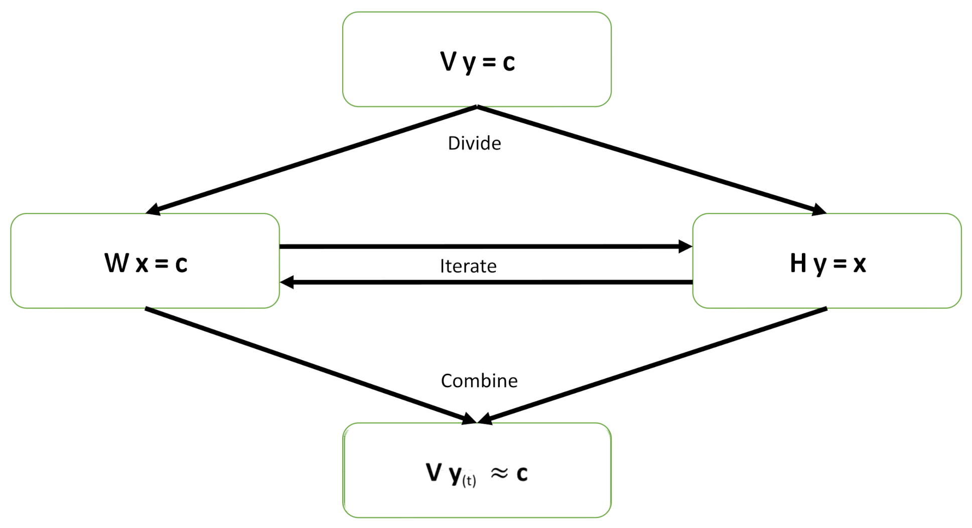
Generally speaking, given a vector $\mathbf{c}$ (dependent variables), we are interested in the linear regression of $\mathbf{V}$ (independent variables) onto $\mathbf{c}$ for a better understanding of the relationship between the dependent and independent variables because many data processing techniques are based on solving a linear-regression problem, for example, beamforming (see [34]), model selection (see [35,36]), robust matrix completion (see [37]), data processing for big data (see [38]), and kernel-based learning (see [39]). Most importantly, the Wiener–Hopf equations are frequently invoked in optimal or adaptive filter design [40]. When tremendous “taps” or “states” are considered, the correlation matrix in the Wiener–Hopf equations becomes very large in dimension. Thus, solving Wiener–Hopf equations with large dimensions is mathematically equivalent to solving a big-data-related linear-regression problem. Because the factorization of a large, big-data-related matrix (or a large correlation matrix) can bring us advantages (as previously discussed), the main contribution of this work is to propose new iterative methods that can work on the factorized matrices instead of the original matrix. By taking such a matrix-factorization approach, one can enjoy the associated benefits in computation, implementation, and representation for solving a linear-regression problem. Our main idea is to utilize a couple of stochastic iterative algorithms for solving the factorized matrices by the Gauss–Seidel algorithm (GSA) in parallel and then combine the individual solutions to form the final approximate solution. There are many existing algorithms to solve large, linear systems of equations, however, the proposed GSA is easier to program and takes less time to compute each iteration compared to existing ones [41,42]. Moreover, we even provide parallel framework to accelerate the proposed GSA. Figure 1 presents a high-level illustration for the proposed new method. This approach can serve as a common framework for solving many large problems by use of the approximate solutions. In this information-technology boom era, problems are often quite large and have to be solved by digital computers subject to finite precision. The proposed new divide-and-iterate method can be applied extensively in data processing for big data. This new approach is different from the conventional divide-and-conquer scheme as there exist no horizontal (mutual iterations among subproblems) computations in the conventional divide-and-conquer approach. Under the same divide-and-iterate approach, this work uses GSA, instead of the Kaczmarz algorithm (KA) [43], to solve factorized subsystems in a parallel method.

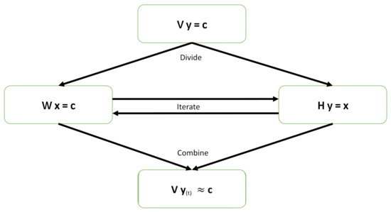
Figure 1. Illustration of the proposed new divide-and-iterate approach.

The rest of this paper is organized as follows. The linear-regression problem and the Gauss–Seidel algorithm are discussed in Section 2. The proposed new iterative approach to solve a factorized system is presented in Section 3. The validation of the convergences of the proposed methods is provided in Section 4. The time- and memory-complexities for our proposed new approach are discussed in Section 5. The numerical experiments for the proposed new algorithms are presented in Section 6. Finally, conclusion will be drawn in Section 7.

2. Solving Linear Regression Using Factorized Matrices and Gauss–Seidel Algorithm

A linear-regression problem (especially involving a large matrix) will be formulated using factorized matrices first in this section. Then, the Gauss–Seidel algorithm will be introduced briefly, as this algorithm needs to be invoked to solve the subproblems involving factorized matrices in parallel. Finally, the individual solutions to these subproblems will be combined to form the final solution.

2.1. Linear Regression: Divide-and-Iterate Approach

A linear regression is given by $\mathbf{V}\mathbf{y}=\mathbf{c},$ where $\mathbf{V}\in {\mathbb{C}}^{m\times n}$ and $\mathbb{C}$ denotes the set of complex numbers. It is equivalent to the following:

$$\begin{array}{c}\hfill \mathbf{V}\mathbf{y}=\mathbf{W}\mathbf{H}\mathbf{y}=\mathbf{c},\end{array}$$

(1)

where the matrix $\mathbf{V}$ is decomposed as the product of the matrix $\mathbf{W}$ and the matrix $\mathbf{H}$, $\mathbf{W}\in {\mathbb{C}}^{m\times k}$, and $\mathbf{H}\in {\mathbb{C}}^{k\times n}$. Generally, the dimension of $\mathbf{V}$ is large in the context of big data. Therefore, it is not practical to solve the original regression problem. We propose to solve the following subproblems alternatively:

$$\begin{array}{ccc}\hfill \mathbf{W}\mathbf{x}& =& \mathbf{c},\hfill \end{array}$$

(2)

and:

$$\begin{array}{ccc}\hfill \mathbf{H}\mathbf{y}& =& \mathbf{x}.\hfill \end{array}$$

(3)

One can obtain the original linear-system solution to Equation (1) by first solving the sub-linear system given by Equation (2) and then substituting the intermediate solution $\mathbf{x}$ into Equation (3) to obtain the final solution $\mathbf{y}$. A linear system $\mathbf{V}\mathbf{y}=\mathbf{c}$ is called consistent if it has at least one solution. On the other hand, it will be called inconsistent if there exists no solution. The sub-linear system can be solved by the Gauss–Seidel algorithm, which will be briefly introduced in the next subsection.

2.2. Gauss–Seidel Algorithm and Its Extensions

The Gauss–Seidel algorithm (GSA) is an iterative algorithm for solving linear equations $\mathbf{V}\mathbf{y}=\mathbf{c}$. It is named after the German mathematicians Carl Friedrich Gauss and Philipp Ludwig von Seidel, and it is similar to the Jacobi method [44]. The randomized version of the Gauss–Seidel method can converge linearly when a consistent system is expected [45].

Given $\mathbf{V}\in {\mathbb{C}}^{m\times n}$ and $\mathbf{c}$ as in Equation (1), the randomized GSA will pick column $j\in \{1,2,\cdots ,n\}$ of $\mathbf{V}$ with probability $\frac{{∥{\mathbf{V}}_{(,j)}∥}_2^2}{{∥\mathbf{A}∥}_F^2}$, where $\mathbb{C}$ denotes the set of complex numbers, ${\mathbf{V}}_{(,j)}$ is the j-th column of the matrix $\mathbf{V}$, ${∥·∥}_F$ is the Frobenius norm, and ${∥·∥}_2$ is the Euclidean norm. Thus, the solution $\mathbf{y}$ will be updated as:

$$\begin{array}{c}\hfill {\mathbf{y}}_t={\mathbf{y}}_{t-1}+\frac{{\mathbf{V}}_{(,j)}^{\ast }(\mathbf{c}-\mathbf{V}{\mathbf{y}}_{t-1})}{{∥{\mathbf{V}}_{(,j)}∥}_2^2}{\mathbf{e}}_{\left(j\right)},\end{array}$$

(4)

where t is the (iteration) index of the solution at the t-th step (iteration), ${\mathbf{e}}_{\left(j\right)}$ is the j-th basis vector (a vector with 1 at the j-th position and 0 otherwise), and ${}^{\ast }$ denotes the Hermitian adjoint of a matrix (vector).

However, the randomized GSA updated by Equation (4) does not converge when the system of equations is inconsistent [45]. To overcome this problem, an extended GSA (EGSA) was proposed in [46]. The EGSA will pick row $i\in \{1,2,\cdots ,m\}$ of $\mathbf{V}$ with probability $\frac{{∥{\mathbf{V}}_{(i,)}∥}_2^2}{{∥\mathbf{V}∥}_F^2}$ and pick column $j\in \{1,2,\cdots ,n\}$ of $\mathbf{V}$ with probability $\frac{{∥{\mathbf{V}}_{(,j)}∥}_2^2}{{∥{\mathbf{V}}_{(,j)}∥}_F^2}$, where ${\mathbf{V}}_{(i,)}$ represents the i-th row of the matrix $\mathbf{V}$. Consequently, the solution $\mathbf{y}$ will be updated as:

$$\begin{array}{c}\hfill {\mathbf{d}}_t={\mathbf{d}}_{t-1}+\frac{{\mathbf{V}}_{(,j)}^{\ast }(\mathbf{c}-\mathbf{V}{\mathbf{d}}_{t-1})}{{∥{\mathbf{V}}_{(,j)}∥}_2^2}{\mathbf{e}}_{\left(j\right)},\end{array}$$

(5)

and:

$$\begin{array}{c}\hfill {\mathbf{y}}_t={\mathbf{y}}_{t-1}+\frac{{\mathbf{V}}_{(i,)}({\mathbf{d}}_t-{\mathbf{y}}_{t-1})}{{∥{\mathbf{V}}_{(i,)}∥}_2^2}{\mathbf{V}}_{(i,)}^{\ast }.\end{array}$$

(6)

When the EGSA is applied for the consistent systems, it behaves exactly like the GSA. For the consistent systems, the EGSA has been shown to converge linearly in expectation to the least-squares solution (${\mathbf{y}}_{opt}={\mathbf{V}}^{†}\mathbf{c}$, where ${}^{†}$ denotes the pseudo-inverse based on the least-squares norm) according to [46].

3. Parallel Random Iterative Approach for Linear Systems

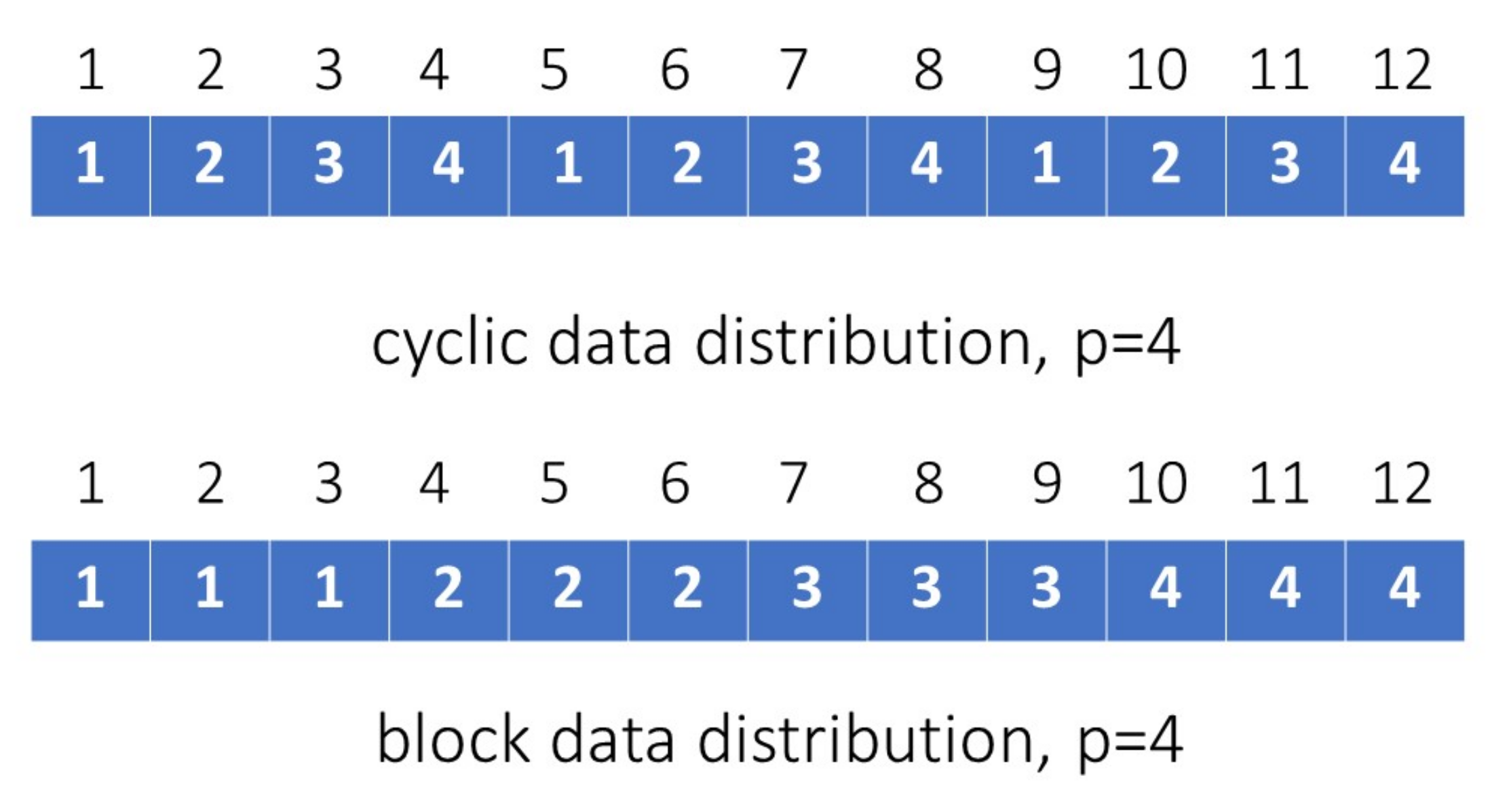
In this section, we will propose a novel parallel approach to deal with vector additions/subtractions and inner-product computations. This new parallel approach can faster the computational speed of the GSA and the EGSA as stated in Section 3.1 and Section 3.2. Suppose that we have p processors (indexed by ${\mathcal{P}}_1$, ${\mathcal{P}}_2$, …, ${\mathcal{P}}_p$) available to carry out vector computations in parallel. The data involved in such computations need be allocated to each processor in balance. Such balanced load of data across all processors can make the best use of resource, maximize the throughput, minimize the computational time, and mitigate the chance of any processor’s overload. Here we propose two strategies to assign data evenly, namely (i) cyclic distribution and (ii) block distribution. For the cyclic distribution, we assign the i-th component of a length-m vector $\mathbf{y}$ to the corresponding processor as follows:

$$\begin{array}{c}\hfill {\mathbf{y}}_{\left(i\right)}\to {\mathcal{P}}_{i|p},\end{array}$$

(7)

where $i|p$ denotes i modulo by p. On the other hand, for block distribution, we assign the i-th component of a length-m vector $\mathbf{x}$ to the corresponding processor as follows:

$$\begin{array}{c}\hfill {\mathbf{y}}_{\left(i\right)}\to {\mathcal{P}}_{⌊\frac{i}{\ell }⌋},\end{array}$$

(8)

where $0\le i<m$, ℓ specifies the block size such that $\ell \stackrel{\mathrm{def}}{=}⌈\frac{m}{p}⌉$, $\lfloor \rfloor$ denotes the integer rounding-down operation, and $\lceil \rceil$ denotes the integer rounding-up operation. The cyclic and block distributions for four processors are illustrated in Figure 2.

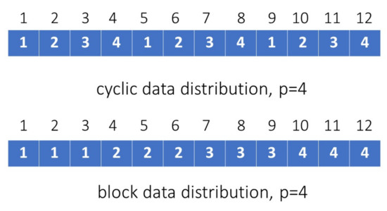
Figure 2. Illustration of the cyclic and block distributions for p = 4.

For example, the parallel computation of an inner product between two vectors using the cyclic distribution is illustrated by Figure 3.

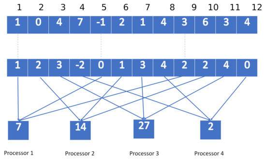
Figure 3. Illustration of an inner-product computation on the parallel platform using cyclic distribution ($p=4$ and $m=12$).

In Figure 3, we illustrate how to undertake a parallel inner product between two vectors $\mathbf{a}\stackrel{\mathrm{def}}{=}[1,0,4,7,-1,2,1,4,3,6,3,4]$ and $\mathbf{b}\stackrel{\mathrm{def}}{=}[1,2,3,-2,0,1,3,4,2,2,4,0]$ via four $(p=4)$ processors. Processor 1 is employed to compute the inner product of the components indexed by 1, 5, and 9, so we obtain $1\times 1+(-1)\times 0+3\times 2=7$; processor 2 is employed to compute the inner product of the components indexed by 2, 6, and 10, so we obtain $0\times 2+2\times 1+6\times 2=14$; processor 3 is employed to compute the inner product of the components indexed by 3, 7, and 11, so we obtain 4 × 3 + 1 × 3 +3 × 4 = 27; finally, processor 4 is employed to compute the inner product of the components indexed by 4, 8, and 12, so we get 7 ×$(-2)$ + 4 × 4 + 4 × 0 = 2. The overall inner product can thus be obtained by adding those above-stated sub-inner products resulting from the four processors.

3.1. Consistent Linear Systems

The parallel random iterative algorithm to solve the original system formulated by Equation (1) is stated by Algorithm 1 if the original system is consistent. The idea here is to solve the sub-system formulated by Equation (2) and the sub-system formulated by Equation (3) alternately using the GSA. The symbols ${\oplus }_p$, ${\ominus }_p$, and ${\odot }_p$ represent parallel vector addition, subtraction, and inner-product, respectively, using p processors. Note that ${\times }_p$ is the operation to scale a vector by a complex value. The parameter $\mathbb{T}$ specifies the number of iterations required to perform the proposed algorithms. This quantity can be determined by the error tolerance of the solution (refer to Section 5.1 for detailed discussion).

Algorithm 1 The Parallel GSA

Result: ${\mathbf{y}}_t$

Input: $\mathbf{W}$, $\mathbf{H}$, $\mathbf{c}$, $\mathbb{T}$; while $t\le \mathbb{T}$ do

Pick up column ${\mathbf{W}}_{(,i)}$ with probability $\frac{{∥{\mathbf{W}}_{(,i)}∥}_2^2}{{∥\mathbf{W}∥}_F^2}$;

Update ${\mathbf{x}}_t={\mathbf{x}}_{t-1}{\oplus }_p\frac{{\mathbf{W}}_{(,i)}^{\ast }{\odot }_p\left(\mathbf{c}{\ominus }_p\mathbf{W}{\mathbf{x}}_{t-1}\right)}{{∥{\mathbf{W}}_{(,i)}∥}_2^2}{\times }_p{\mathbf{e}}_{\left(i\right)}$;

Pick up column ${\mathbf{H}}_{(,j)}$ with probability $\frac{{∥{\mathbf{H}}_{(,j)}∥}_2^2}{{∥\mathbf{H}∥}_F^2}$;

Update ${\mathbf{y}}_t={\mathbf{y}}_{t-1}{\oplus }_p\frac{{\mathbf{H}}_{(,j)}^{\ast }{\odot }_p\left({\mathbf{x}}_t{\ominus }_p\mathbf{H}{\mathbf{y}}_{t-1}\right)}{{∥{\mathbf{H}}_{(,j)}∥}_2^2}{\times }_p{\mathbf{e}}_{\left(j\right)}$;

end

3.2. Inconsistent Linear Systems

If the original system formulated by Equation (1) is not consistent, Algorithm 2 is proposed to solve it instead. Algorithm 2 below is based on the EGSA.

Algorithm 2 The Parallel EGSA

Result: ${\mathbf{y}}_t$ Input: $\mathbf{W}$, $\mathbf{H}$, $\mathbf{c}$, $\mathbb{T}$

while$t\le \mathbb{T}$do

Pick up column ${\mathbf{W}}_{(,i)}$ with probability $\frac{{∥{\mathbf{W}}_{(,i)}∥}_2^2}{{∥\mathbf{W}∥}_F^2}$

Update ${\mathbf{d}}_t={\mathbf{d}}_{t-1}{\oplus }_p\frac{{\mathbf{W}}_{(,i)}^{\ast }{\odot }_p\left(\mathbf{c}{\ominus }_p\mathbf{V}{\mathbf{d}}_{t-1}\right)}{{∥{\mathbf{W}}_{(,i)}∥}_2^2}{\times }_p{\mathbf{e}}_{\left(i\right)}$

Pick up row ${\mathbf{W}}_{(l,)}$ with probability $\frac{{∥{\mathbf{W}}_{(l,)}∥}_2^2}{{∥\mathbf{W}∥}_F^2}$

Update ${\mathbf{x}}_t={\mathbf{x}}_{t-1}{\oplus }_p\frac{{\mathbf{W}}_{(l,)}{\odot }_p\left({\mathbf{d}}_t{\ominus }_p{\mathbf{x}}_{t-1}\right)}{{∥{\mathbf{W}}_{(l,)}∥}_2^2}{\times }_p{\mathbf{W}}_{(l,)}^{\ast }$

Pick up column ${\mathbf{H}}_{(,j)}$ with probability $\frac{{∥{\mathbf{H}}_{(,j)}∥}_2^2}{{∥\mathbf{H}∥}_F^2}$

Update ${\mathbf{y}}_t={\mathbf{y}}_{t-1}{\oplus }_p\frac{{\mathbf{H}}_{(,j)}^{\ast }{\odot }_p\left({\mathbf{x}}_t{\ominus }_p\mathbf{H}{\mathbf{y}}_{t-1}\right)}{{∥{\mathbf{H}}_{(,j)}∥}_2^2}{\times }_p{\mathbf{e}}_{\left(j\right)}$

end

4. Convergence Studies

The convergence studies for the two algorithms proposed in Section 3 are manifested by Theorem 1 for consistent systems and Theorem 2 for inconsistent systems. The necessary lemmas for establishing the main theorems discussed in Section 4.2 are first presented in Section 4.1. All proofs will be written using vector operations without the subscript p because the parallel computations for vector operations should lead to the same results regardless of the processor index p. Without loss of generality, the instances of subscript p indexed in Algorithms 1 and 2 are simply used to indicate that those computations can be carried out in parallel.

4.1. Auxiliary Lemmas

We define the metric ${\varrho }_{\mathbf{A}}$ for a matrix $\mathbf{A}$ as:

$$\begin{array}{c}\hfill {\varrho }_{\mathbf{A}}\stackrel{\mathrm{def}}{=}1-\frac{{\sigma }_{min}^2\left(\mathbf{A}\right)}{{\parallel \mathbf{A}\parallel }_{\mathrm{F}}^2},\end{array}$$

(9)

where ${\sigma }_{min}\left(\mathbf{A}\right)$ denotes the minimum nontrivial singular value of the matrix $\mathbf{A}$ and $0<{\sigma }_{min}\left(\mathbf{A}\right)<1$. We present the following lemma, which establishes an identity related to the error bounds of our proposed iterative algorithms.

Lemma 1.

Let $\mathbf{A}$ be a nonzero real matrix. For any vector $\mathbf{v}$ in the range of $\mathbf{A}$, i.e., $\mathbf{v}$ can be obtained by a linear combination of $\mathbf{A}$’s columns (taking columns as vectors), we have:

$$\begin{array}{c}\hfill {\mathbf{v}}^T\left(I-\frac{\mathbf{A}{\mathbf{A}}^{\mathbf{T}}}{{∥\mathbf{A}∥}_F^2}\right)\mathbf{v}\le {\varrho }_{\mathbf{A}}{∥\mathbf{v}∥}_2^2.\end{array}$$

(10)

Proof. 

Because the singular values of $\mathbf{A}$ and ${\mathbf{A}}^T$ are the same and ${\sigma }_i\left(\mathbf{A}{\mathbf{A}}^T\right)\ge {\sigma }_{min}^2\left(\mathbf{A}\right)$ where the subscript i denotes the i-th largest singular value in magnitude, Lemma 1 is proven. □

Since the original solution to Equation (1) can be facilitated from solving the factorized linear systems, Lemma 2 below can be utilized to bound the error arising from the solutions to the factorized sub-systems at each iteration.

Lemma 2.

The expected squared-norm for $\mathbf{H}{\mathbf{y}}_t-\mathbf{H}{\mathbf{y}}_{opt}$, or the error between the result at the t-th iteration and the optimal solution conditional on the first t iterations, is given by:

$$\begin{array}{c}\hfill {\mathbb{E}}_t\left[{∥\mathbf{H}{\mathbf{y}}_{t+1}-\mathbf{H}{\mathbf{y}}_{\mathrm{opt}}∥}_2^2\right]\le {\varrho }_{\mathbf{H}}{∥\mathbf{H}{\mathbf{y}}_t-\mathbf{H}{\mathbf{y}}_{\mathrm{opt}}∥}_2^2+{\mathbb{E}}_{t,\mathbf{x}}\left[{∥{\mathbf{x}}_{t+1}-{\mathbf{x}}_{\mathrm{opt}}∥}_2^2\right]\end{array}$$

(11)

where the subscript $\mathbf{x}$ of the statistical expectation operator ${\mathbb{E}}_{t,\mathbf{x}}\left[\right]$ indicates that the expectation should be taken over the random variable $\mathbf{x}$.

Proof. 

Let ${\widehat{\mathbf{y}}}_{t+1}$ be the one-step update in the GSA, so ${\widehat{\mathbf{y}}}_{t+1}={\mathbf{y}}_t+\frac{{\mathbf{H}}_{(,j)}^{\ast }({\mathbf{x}}_{opt}-\mathbf{H}{\mathbf{y}}_t)}{{∥{\mathbf{H}}_{(,j)}∥}_2^2}{\mathbf{e}}_{\left(j\right)}$ and: ${\mathbf{y}}_{t+1}={\mathbf{y}}_t+\frac{{\mathbf{H}}_{(,j)}^{\ast }({\mathbf{x}}_t-\mathbf{H}{\mathbf{y}}_t)}{{∥{\mathbf{H}}_{(,j)}∥}_2^2}{\mathbf{e}}_{\left(j\right)}$.

Then we have:

$$\begin{array}{cc}\hfill & {\mathbb{E}}_t\left[{∥\mathbf{H}{\mathbf{y}}_{t+1}-\mathbf{H}{\mathbf{y}}_{\mathrm{opt}}∥}_2^2\right]\hfill \\ \hfill & ={}_{\left(1\right)}{\mathbb{E}}_t\left[{∥\mathbf{H}{\mathbf{y}}_{t+1}-\mathbf{H}{\mathbf{y}}_{\mathrm{opt}}+\mathbf{H}{\widehat{\mathbf{y}}}_{t+1}-\mathbf{H}{\widehat{\mathbf{y}}}_{t+1}∥}_2^2\right]\hfill \\ \hfill & ={}_{\left(2\right)}{\mathbb{E}}_t\left[{∥\mathbf{H}{\widehat{\mathbf{y}}}_{t+1}-\mathbf{H}{\mathbf{y}}_{\mathrm{opt}}∥}_2^2\right]+{\mathbb{E}}_t\left[{∥\mathbf{H}{\mathbf{y}}_{t+1}-\mathbf{H}{\widehat{\mathbf{y}}}_{t+1}∥}_2^2\right]\hfill \\ \hfill & ={}_{\left(3\right)}{\mathbb{E}}_t\left[{∥\mathbf{H}{\mathbf{y}}_t-\mathbf{H}{\mathbf{y}}_{\mathrm{opt}}∥}_2^2\right]-{\mathbb{E}}_t\left[{∥\mathbf{H}{\widehat{\mathbf{y}}}_{t+1}-{\mathbf{Hy}}_t∥}_2^2\right]+{\mathbb{E}}_t\left[{∥\mathbf{H}{\mathbf{y}}_{t+1}-\mathbf{H}{\widehat{\mathbf{y}}}_{t+1}∥}_2^2\right]\hfill \\ \hfill & ={}_{\left(4\right)}{\parallel \mathbf{H}{\mathbf{y}}_t-\mathbf{H}{\mathbf{y}}_{\mathrm{opt}}\parallel }_2^2-{\mathbb{E}}_t\left[\frac{|{\mathbf{H}}_{(,j)}^{\ast }\mathbf{H}{\mathbf{y}}_{\mathrm{opt}}-{\mathbf{H}}_{(,j)}^{\ast }{\mathbf{Hy}}_t{|}^2}{{∥{\mathbf{H}}_{(,j)}^{\ast }∥}_2^2}\right]+{\mathbb{E}}_t\left[\frac{|{\mathbf{H}}_{(,j)}^{\ast }{\mathbf{x}}_{t+1}-{\mathbf{H}}_{(,j)}^{\ast }{\mathbf{x}}_{\mathrm{opt}}{|}^2}{{∥{\mathbf{H}}_{(,j)}^{\ast }∥}_2^2}\right]\hfill \\ \hfill & ={}_{\left(5\right)}{∥\mathbf{H}{\mathbf{y}}_t-\mathbf{H}{\mathbf{y}}_{\mathrm{opt}}∥}_2^2-{\mathbb{E}}_{t,\mathbf{y}}\left[\frac{|{\mathbf{H}}_{(,j)}^{\ast }\mathbf{H}{\mathbf{y}}_{\mathrm{opt}}-{\mathbf{H}}_{(,j)}^{\ast }\mathbf{H}{\mathbf{y}}_t{|}^2}{{∥{\mathbf{H}}_{(,j)}^{\ast }∥}_2^2}\right]+{\mathbb{E}}_{t,\mathbf{x}}\left\{{\mathbb{E}}_{t,\mathbf{y}}\left[\frac{|{\mathbf{H}}_{(,j)}^{\ast }{\mathbf{x}}_{t+1}-{\mathbf{H}}_{(,j)}^{\ast }{\mathbf{x}}_{\mathrm{opt}}{|}^2}{{∥{\mathbf{H}}_{(,j)}^{\ast }∥}_2^2}\right]\right\}\hfill \\ \hfill & ={}_{\left(6\right)}{∥\mathbf{H}{\mathbf{y}}_t-\mathbf{H}{\mathbf{y}}_{\mathrm{opt}}∥}_2^2-\frac{{∥{\mathbf{H}}^{\ast }\left(\mathbf{H}{\mathbf{y}}_{\mathrm{opt}}-\mathbf{H}{\mathbf{y}}_t\right)∥}_2^2}{{\parallel \mathbf{H}\parallel }_{\mathrm{F}}^2}+\frac{{\mathbb{E}}_{t,\mathbf{x}}\left[{∥{\mathbf{H}}^{\ast }\left({\mathbf{x}}_{t+1}-{\mathbf{x}}_{\mathrm{opt}}\right)∥}_2^2\right]}{{\parallel \mathbf{H}\parallel }_{\mathrm{F}}^2}\hfill \\ \hfill & {\le }_{\left(7\right)}{∥\mathbf{H}{\mathbf{y}}_t-\mathbf{H}{\mathbf{y}}_{\mathrm{opt}}∥}_2^2-\frac{{\sigma }_{min}^2\left(\mathbf{H}\right)}{{\parallel \mathbf{H}\parallel }_{\mathrm{F}}^2}{∥\mathbf{H}{\mathbf{y}}_t-\mathbf{H}{\mathbf{y}}_{\mathrm{opt}}∥}_2^2+\frac{{\mathbb{E}}_{t,\mathrm{x}}\left[{∥{\mathbf{H}}^{\ast }\left({\mathbf{x}}_{t+1}-{\mathbf{x}}_{\mathrm{opt}}\right)∥}_2^2\right]}{{\parallel \mathbf{H}\parallel }_{\mathrm{F}}^2}\hfill \\ \hfill & ={}_{\left(8\right)}\varrho \mathbf{H}{∥\mathbf{H}{\mathbf{y}}_t-\mathbf{H}{\mathbf{y}}_{\mathrm{opt}}∥}_2^2+\frac{{\mathbb{E}}_{t,\mathbf{x}}\left[{∥{\mathbf{H}}^{\ast }\left({\mathbf{x}}_{t+1}-{\mathbf{x}}_{\mathrm{opt}}\right)∥}_2^2\right]}{{\parallel \mathbf{H}\parallel }_{\mathrm{F}}^2}\hfill \\ \hfill & {\le }_{\left(9\right)}\varrho \mathbf{H}{∥\mathbf{H}{\mathbf{y}}_t-\mathbf{H}{\mathbf{y}}_{\mathrm{opt}}∥}_2^2+{\mathbb{E}}_{t,\mathrm{x}}\left[{∥{\mathbf{x}}_{t+1}-{\mathbf{x}}_{\mathrm{opt}}∥}_2^2\right].\hfill \\ \hfill \end{array}$$

(12)

The equality ${=}_{\left(1\right)}$ results from adding and subtracting the same term “$\mathbf{H}{\widehat{\mathbf{y}}}_{t+1}$”. The equality ${=}_{\left(2\right)}$ holds because $\mathbf{H}{\widehat{\mathbf{y}}}_{t+1}-\mathbf{H}{\mathbf{y}}_{opt}$ and $\mathbf{H}{\mathbf{y}}_{t+1}-\mathbf{H}{\widehat{\mathbf{y}}}_{t+1}$ are orthogonal to each other. The equality ${=}_{\left(3\right)}$ comes from Pythagoras’ Theorem since $\mathbf{H}{\widehat{\mathbf{y}}}_{t+1}-\mathbf{H}{\mathbf{y}}_{opt}$ and $\mathbf{H}{\widehat{\mathbf{y}}}_{t+1}-\mathbf{H}{\mathbf{y}}_t$ are orthogonal to each other. The proof of the orthogonality between $\mathbf{H}{\widehat{\mathbf{y}}}_{t+1}$−$\mathbf{H}{\mathbf{y}}_{opt}$ and $\mathbf{H}{\widehat{\mathbf{y}}}_{t+1}$−$\mathbf{H}{\mathbf{y}}_t$ is presented as follows: $(\mathbf{H}{\widehat{\mathbf{y}}}_{t+1}$−$\mathbf{H}{\mathbf{y}}_t)$ is parallel to ${\mathbf{H}}_{(,j)}$ and $(\mathbf{H}{\widehat{\mathbf{y}}}_{t+1}$−$\mathbf{H}{\mathbf{y}}_{opt})$ is perpendicular to ${\mathbf{H}}_{(,j)}$ because:

$$\begin{array}{cc}\hfill {\mathbf{H}}_{(,j)}& (\mathbf{H}{\widehat{\mathbf{y}}}_{t+1}-\mathbf{H}{\mathbf{y}}_{\mathrm{opt}})\hfill \\ \hfill & ={\mathbf{H}}_{(,j)}\left[\mathbf{H}\left({\mathbf{y}}_t+\frac{{\mathbf{H}}_{(,j)}^{\ast }\left({\mathbf{x}}_{\mathrm{opt}}-\mathbf{H}{\mathbf{y}}_t\right)}{{∥{\mathbf{H}}_{(,j)}∥}_2^2}{\mathbf{e}}_{\left(j\right)}\right)-\mathbf{H}{\mathbf{y}}_{\mathrm{opt}}\right]\hfill \\ \hfill & ={\mathbf{H}}_{(,j)}\mathbf{H}{\mathbf{y}}_t+{\mathbf{H}}_{(,j)}\mathbf{H}{\mathbf{y}}_{\mathrm{opt}}-{\mathbf{H}}_{(,j)}\mathbf{H}{\mathbf{y}}_t-{\mathbf{H}}_{(,j)}\mathbf{H}{\mathbf{y}}_{\mathrm{opt}}=0.\hfill \end{array}$$

(13)

Therefore, $\mathbf{H}{\widehat{\mathbf{y}}}_{t+1}$−$\mathbf{H}{\mathbf{y}}_{opt}$ and $\mathbf{H}{\widehat{\mathbf{y}}}_{t+1}$−$\mathbf{H}{\mathbf{y}}_t$ are orthogonal to each other. The relation $\mathbf{H}{\mathbf{y}}_{opt}={\mathbf{x}}_{opt}$ is used to establish the identity ${=}_{\left(4\right)}$. Recall that the expectation ${\mathbb{E}}_t\left[\right]$ is conditional on the first t iterations. The law of iterated expectations in [47] is thereby applied here to establish the equality ${=}_{\left(5\right)}$. Since the probability of selecting the column ${\mathbf{H}}_{(,j)}$ is $\frac{{∥{\mathbf{H}}_{(,j)}∥}_2^2}{{∥\mathbf{H}∥}_F^2}$, we can have the equality ${=}_{\left(6\right)}$. The inequality ${\le }_{\left(7\right)}$ comes from the fact that ${∥{\mathbf{H}}^{\ast }(\mathbf{H}{\mathbf{y}}_{opt}-\mathbf{H}{\mathbf{y}}_t)∥}_2^2\ge {\varrho }_{\mathbf{H}}{∥\mathbf{H}{\mathbf{y}}_t-\mathbf{H}{\mathbf{y}}_{opt}∥}_2^2$. The equality ${=}_{\left(8\right)}$ results from the definition of ${\varrho }_{\mathbf{H}}$ in Equation (9). Finally, the inequality ${\le }_{\left(9\right)}$ comes from the fact that ${∥\mathbf{A}\mathbf{x}∥}_2^2\le {∥\mathbf{A}∥}_F^2{∥\mathbf{x}∥}_2^2$ (according to the Cauchy–Schwarz inequality) for the matrix $\mathbf{A}\in {\mathbb{C}}^{m\times n}$ and the vector $\mathbf{x}\in {\mathbb{C}}^{n\times 1}$. □

Lemma 3.

Consider a linear, consistent system $\mathbf{V}\mathbf{y}=\mathbf{c}$ where $\mathbf{V}$ has the dimension $m\times n$. If the Gauss–Siedel algorithm (GSA) with an initial guess ${\mathbf{y}}_0\in {\mathbb{R}}^n$ ($\mathbb{R}$ denotes the set of real numbers) is applied to solve such a linear, consistent system, the expected squared-norm for ${\mathbf{y}}_t-{\mathbf{y}}_{opt}$ can be bounded as follows:

$$\begin{array}{c}\hfill \mathbb{E}\left[{∥{\mathbf{y}}_t-{\mathbf{y}}_{opt}∥}_2^2\right]\le {\rho }_{\mathbf{V}}^t{∥{\mathbf{y}}_0-{\mathbf{y}}_{opt}∥}_2^2.\end{array}$$

(14)

Proof. 

See Theorem 4.2 in [45]. □

The following lemma is presented to bound the iterative results for solving an inconsistent system using the extended Gauss–Siedel algorithm (EGSA).

Lemma 4.

Consider a linear, inconsistent system $\mathbf{V}\mathbf{y}=\mathbf{c}$. If the extended Gauss–Siedel algorithm (EGSA) with an initial guess ${\mathbf{y}}_0$ within the range of ${\mathbf{V}}^T$ and ${\mathbf{d}}_0\in {\mathbb{R}}^n$ is applied to solve such a linear, inconsistent system, the expected squared-norm for ${\mathbf{y}}_s-{\mathbf{y}}_{opt}$ can be bounded as follows:

$$\begin{array}{ccc}\hfill \mathbb{E}\left[{∥{\mathbf{y}}_t-{\mathbf{y}}_{opt}∥}_2^2\right]& \le & {\varrho }_{\mathbf{V}}^t{∥{\mathbf{y}}_0-{\mathbf{y}}_{opt}∥}_2^2+\hfill \\ & & \frac{t{\varrho }_{\mathbf{V}}^t}{{∥\mathbf{V}∥}_F^2}{∥\mathbf{V}{\mathbf{d}}_0-\mathbf{V}{\mathbf{y}}_{opt}∥}_2^2.\hfill \end{array}$$

(15)

Proof. 

Since:

$$\begin{array}{cc}\hfill {\mathbf{y}}_t-{\mathbf{y}}_{\mathrm{opt}}=& {\mathbf{y}}_{t-1}+\frac{{\mathbf{V}}_{(l,)}\left({\mathbf{d}}_t-{\mathbf{y}}_{t-1}\right)}{{∥{\mathbf{V}}_{(l,)}∥}_2^2}{\mathbf{V}}_{(l,)}^{\ast }-{\mathbf{y}}_{\mathrm{opt}}\hfill \\ \hfill =& \left[\mathbf{I}-\frac{{\mathbf{V}}_{(l,)}^{\ast }{\mathbf{V}}_{(l,)}}{{∥{\mathbf{V}}_{(l,)}∥}_2^2}\right]{\mathbf{y}}_{t-1}+\frac{{\mathbf{V}}_{(l,)}^{\ast }{\mathbf{V}}_{(l,)}}{{∥{\mathbf{V}}_{(l,)}∥}_2^2}{\mathbf{d}}_t-{\mathbf{y}}_{\mathrm{opt}}\hfill \\ \hfill =& \left[\mathbf{I}-\frac{{\mathbf{V}}_{(l,)}^{\ast }{\mathbf{V}}_{(l,)}}{{∥{\mathbf{V}}_{(l,)}∥}_2^2}\right]\left({\mathbf{y}}_{t-1}-{\mathbf{y}}_{\mathrm{opt}}\right)+\frac{{\mathbf{V}}_{(l,)}^{\ast }{\mathbf{V}}_{(l,)}}{{∥{\mathbf{V}}_{(l,)}∥}_2^2}\left({\mathbf{d}}_t-{\mathbf{y}}_{\mathrm{opt}}\right)\hfill \end{array}$$

(16)

$${\left[\frac{{\mathbf{V}}_{(l,)}^{\ast }{\mathbf{V}}_{(l,)}}{{∥{\mathbf{V}}_{(l,)}∥}_2^2}\right]}^2=\frac{{\mathbf{V}}_{(l,)}^{\ast }{\mathbf{V}}_{(l,)}}{{∥{\mathbf{V}}_{(l,)}∥}_2^2}$$

(17)

and:

$${\left({\mathbf{d}}_t-{\mathbf{y}}_{\mathrm{opt}}\right)}^T\frac{{\mathbf{V}}_{(l,)}^{\ast }{\mathbf{V}}_{(l,)}}{{∥{\mathbf{V}}_{(l,)}∥}_2^2}\left[\mathbf{I}-\frac{{\mathbf{V}}_{(l,)}^{\ast }{\mathbf{V}}_{(l,)}}{{∥{\mathbf{V}}_{(l,)}∥}_2^2}\right]\times \left({\mathbf{y}}_{t-1}-{\mathbf{y}}_{\mathrm{opt}}\right)=0$$

(18)

we have the following:

$${∥{\mathbf{y}}_t-{\mathbf{y}}_{\mathrm{opt}}∥}_2^2={∥\left[\mathbf{I}-\frac{{\mathbf{V}}_{(l,)}^{\ast }{\mathbf{V}}_{(l,)}}{{∥{\mathbf{V}}_{(l,)}∥}_2^2}\right]\left({\mathbf{y}}_{t-1}-{\mathbf{y}}_{\mathrm{opt}}\right)∥}_2^2+{∥\frac{{\mathbf{V}}_{(l,)}^{\ast }{\mathbf{V}}_{(l,)}}{{∥{\mathbf{V}}_{(l,)}∥}_2^2}\left({\mathbf{d}}_t-{\mathbf{y}}_{\mathrm{opt}}\right)∥}_2^2$$

(19)

The expectation of the first term in Equation (19) can be bounded as:

$$\begin{array}{cc}\hfill & {\mathbb{E}}_{t-1}\left[{∥\left(\mathbf{I}-\frac{{\mathbf{V}}_{(l,)}^{\ast }{\mathbf{V}}_{(l,)}}{{∥{\mathbf{V}}_{(l,)}∥}_2^2}\right)\left({\mathbf{y}}_{t-1}-{\mathbf{y}}_{\mathrm{opt}}\right)∥}_2^2\right]\hfill \\ \hfill & ={\mathbb{E}}_{t-1}\left[{\left({\mathbf{y}}_{t-1}-{\mathbf{y}}_{\mathrm{opt}}\right)}^T{\left(\mathbf{I}-\frac{{\mathbf{V}}_{(l,)}^{\ast }{\mathbf{V}}_{(l,)}}{{∥{\mathbf{V}}_{(l,)}∥}_2^2}\right)}^2\left({\mathbf{y}}_{t-1}-{\mathbf{y}}_{\mathrm{opt}}\right)\right]\hfill \\ \hfill & ={\mathbb{E}}_{t-1}\left[{\left({\mathbf{y}}_{t-1}-{\mathbf{y}}_{\mathrm{opt}}\right)}^T\left(\mathbf{I}-\frac{{\mathbf{V}}_{(l,)}^{\ast }{\mathbf{V}}_{(l,)}}{{∥{\mathbf{V}}_{(l,)}∥}_2^2}\right)\left({\mathbf{y}}_{t-1}-{\mathbf{y}}_{\mathrm{opt}}\right)\right]\hfill \\ \hfill & ={\left({\mathbf{y}}_{t-1}-{\mathbf{y}}_{\mathrm{opt}}\right)}^T\left(\mathbf{I}-\frac{{\mathbf{V}}_{(l,)}^{\ast }{\mathbf{V}}_{(l,)}}{{∥{\mathbf{V}}_{(l,)}∥}_2^2}\right)\left({\mathbf{y}}_{t-1}-{\mathbf{y}}_{\mathrm{opt}}\right)\hfill \\ \hfill & \le {\varrho }_{\mathbf{V}}{∥{\mathbf{y}}_{t-1}-{\mathbf{y}}_{\mathrm{opt}}∥}_2^2\hfill \end{array}$$

(20)

Then, we have:

$$\mathbb{E}\left[{∥\left(\mathbf{I}-\frac{{\mathbf{V}}_{(l,)}^{\ast }{\mathbf{V}}_{(l,)}}{{∥{\mathbf{V}}_{(l,)}∥}_2^2}\right)\left({\mathbf{y}}_{t-1}-{\mathbf{y}}_{\mathrm{opt}}\right)∥}_2^2\right]\le {\varrho }_{\mathbf{V}}\mathbb{E}\left[{∥{\mathbf{y}}_{t-1}-{\mathbf{y}}_{\mathrm{opt}}∥}_2^2\right]$$

(21)

The expectation of the second term in Equation (19) is given by:

$$\begin{array}{cc}\hfill & {\mathbb{E}}_{t-1}\left[{∥\frac{{\mathbf{V}}_{(l,)}^{\ast }{\mathbf{V}}_{(l,)}}{{∥{\mathbf{V}}_{(l,)}∥}_2^2}\left({\mathbf{d}}_t-{\mathbf{y}}_{\mathrm{opt}}\right)∥}_2^2\right]\hfill \\ \hfill & ={\mathbb{E}}_{t-1}\left[{\left({\mathbf{d}}_t-{\mathbf{y}}_{\mathrm{opt}}\right)}^T{\left(\frac{{\mathbf{V}}_{(l,)}^{\ast }{\mathbf{V}}_{(l,)}}{{∥{\mathbf{V}}_{(l,)}∥}_2^2}\right)}^2\left({\mathbf{d}}_t-{\mathbf{y}}_{\mathrm{opt}}\right)\right]\hfill \\ \hfill & =\left(1\right){\mathbb{E}}_{t-1,(,i)}\left\{{\mathbb{E}}_{t-1,(l,)}\left[{\left({\mathbf{d}}_t-{\mathbf{y}}_{\mathrm{opt}}\right)}^T\frac{{\mathbf{V}}_{(l,)}^{\ast }{\mathbf{V}}_{(l,)}}{{∥{\mathbf{V}}_{(l,)}∥}_2^2}\left({\mathbf{d}}_t-{\mathbf{y}}_{\mathrm{opt}}\right)\right]\right\}\hfill \\ \hfill & ={}_{\left(2\right)}{\mathbb{E}}_{t-1,(,i)}\left[{\left({\mathbf{d}}_t-{\mathbf{y}}_{\mathrm{opt}}\right)}^T\frac{{\mathbf{V}}^{\ast }\mathbf{V}}{{\parallel \mathbf{V}\parallel }_{\mathrm{F}}^2}\left({\mathbf{d}}_t-{\mathbf{y}}_{\mathrm{opt}}\right)\right]\hfill \\ \hfill & =\frac{{\mathbb{E}}_{t-1}\left[{∥\mathbf{V}{\mathbf{d}}_t-\mathbf{V}{\mathbf{y}}_{\mathrm{opt}}∥}_2^2\right]}{{\parallel \mathbf{V}\parallel }_{\mathrm{F}}^2}\hfill \end{array}$$

(22)

where the equality ${=}_{\left(1\right)}$ comes from the law of iterated expectations again for the conditional expectations ${\mathbb{E}}_{t-1,(,i)}\left[\right]$ (conditional on the i-th column at the $(t-1)$-th iteration) and ${\mathbb{E}}_{t-1,(l,)}\left[\right]$ (conditional on the l-th row at the $(t-1)$-th iteration), and the equality ${=}_{\left(2\right)}$ comes from the probability of selecting the l-th row to be $\frac{{∥{\mathbf{V}}_{(l,)}∥}_2^2}{{∥\mathbf{V}∥}_F^2}$.

From the GSA update rule, we can have the following inequality:

$$\begin{array}{cc}\hfill & {\mathbb{E}}_{t-1}\left[{∥\frac{{\mathbf{V}}_{(l,)}^{\ast }{\mathbf{V}}_{(l,)}}{{∥{\mathbf{V}}_{(l,)}∥}_2^2}\left({\mathbf{d}}_t-{\mathbf{y}}_{\mathrm{opt}}\right)∥}_2^2\right]=\frac{{\mathbb{E}}_{t-1}\left[{∥\mathbf{V}{\mathbf{d}}_t-\mathbf{V}{\mathbf{y}}_{\mathrm{opt}}∥}_2^2\right]}{{\parallel \mathbf{V}\parallel }_{\mathrm{F}}^2}\hfill \\ \hfill & =\frac{{\mathbb{E}}_{t-1}\left[{\left(\mathbf{V}{\mathbf{d}}_t-\mathbf{V}{\mathbf{y}}_{\mathrm{opt}}\right)}^T\left(\mathbf{V}{\mathbf{d}}_t-\mathbf{V}{\mathbf{y}}_{\mathrm{opt}}\right)\right]}{{\parallel \mathbf{V}\parallel }_{\mathrm{F}}^2}\hfill \\ \hfill & =\left(1\right)\frac{{\mathbb{E}}_{t-1}\left[{\left(\mathbf{V}{\mathbf{d}}_{t-1}-\mathbf{V}{\mathbf{y}}_{\mathrm{opt}}\right)}^T{\left(\mathbf{I}-\frac{{\mathbf{V}}_{(,i)}^{\ast }{\mathbf{V}}_{(,i)}}{{∥{\mathbf{V}}_{(,i)}∥}_2^2}\right)}^2\left(\mathbf{V}{\mathbf{d}}_{t-1}-\mathbf{V}{\mathbf{y}}_{\mathrm{opt}}\right)\right]}{{\parallel \mathbf{V}\parallel }_{\mathrm{F}}^2}\hfill \\ \hfill & =\left(2\right){\mathbb{E}}_{t-1}\left[{\left(\mathbf{V}{\mathbf{d}}_{t-1}-\mathbf{V}{\mathbf{y}}_{\mathrm{opt}}\right)}^T\left(\mathbf{I}-\frac{{\mathbf{V}}_{(,i)}^{\ast }{\mathbf{V}}_{(,i)}}{{∥{\mathbf{V}}_{(,i)}∥}_2^2}\right)\right.\left.\times \left(\mathbf{V}{\mathbf{d}}_{t-1}-\mathbf{V}{\mathbf{y}}_{\mathrm{opt}}\right)\right]/{\parallel \mathbf{V}\parallel }_{\mathrm{F}}^2\hfill \\ \hfill & =\frac{{\left(\mathbf{V}{\mathbf{d}}_{t-1}-\mathbf{V}{\mathbf{y}}_{\mathrm{opt}}\right)}^T\left(\mathbf{I}-\frac{{\mathbf{V}}_{(,i)}^{\ast }{\mathbf{V}}_{(,i)}}{{∥{\mathbf{V}}_{(,i)}∥}_2^2}\right)\left(\mathbf{V}{\mathbf{d}}_{t-1}-\mathbf{V}{\mathbf{y}}_{\mathrm{opt}}\right)}{{\parallel \mathbf{V}\parallel }_{\mathrm{F}}^2}\hfill \\ \hfill & {\le }_{\left(3\right)}\frac{\varrho \mathbf{V}{∥\mathbf{V}{\mathbf{d}}_{t-1}-\mathbf{V}{\mathbf{y}}_{\mathrm{opt}}∥}_2^2}{{\parallel \mathbf{V}\parallel }_{\mathrm{F}}^2}\hfill \end{array}$$

(23)

where the equality ${=}_{\left(1\right)}$ is established by applying the GSA one-step update, and the equality ${=}_{\left(2\right)}$ is based on the fact that ${\left(\mathbf{I}-\frac{{\mathbf{V}}_{(,i)}^{\ast }{\mathbf{V}}_{(,i)}}{{∥{\mathbf{V}}_{(,i)}∥}_2^2}\right)}^2=\mathbf{I}-\frac{{\mathbf{V}}_{(,i)}^{\ast }{\mathbf{V}}_{(,i)}}{{∥{\mathbf{V}}_{(,i)}∥}_2^2})$. The inequality ${\le }_{\left(3\right)}$ comes from Lemma 1. Based on this inequality and the law of iterated expectations, the expectation of the second term in Equation (19) can be bounded as:

$$\mathbb{E}\left[{∥\frac{{\mathbf{V}}_{(l,)}^{\ast }{\mathbf{V}}_{(l,)}}{{∥{\mathbf{V}}_{(l,)}∥}_2^2}\left({\mathbf{d}}_t-{\mathbf{y}}_{\mathrm{opt}}\right)∥}_2^2\right]\le \frac{{\varrho }_{\mathbf{V}}^t{∥\mathbf{V}{\mathbf{d}}_0-\mathbf{V}{\mathbf{y}}_{\mathrm{opt}}∥}_2^2}{{\parallel \mathbf{V}\parallel }_{\mathrm{F}}^2}$$

(24)

According to Equations (19), (21) and (24), we have:

$$\begin{array}{cc}\hfill \mathbb{E}\left[{∥{\mathbf{y}}_t-{\mathbf{y}}_{\mathrm{opt}}∥}_2^2\right]& =\mathbb{E}\left[{∥\left(\mathbf{I}-\frac{{\mathbf{V}}_{(l,)}^{\ast }{\mathbf{V}}_{(l,)}}{{∥{\mathbf{V}}_{(l,)}∥}_2^2}\right)\left({\mathbf{y}}_{t-1}-{\mathbf{y}}_{\mathrm{opt}}\right)∥}_2^2\right]\hfill \\ \hfill & +\mathbb{E}\left[{∥\frac{{\mathbf{V}}_{(l,)}^{\ast }{\mathbf{V}}_{(l,)}}{{∥{\mathbf{V}}_{(l,)}∥}_2^2}\left({\mathbf{d}}_t-{\mathbf{y}}_{\mathrm{opt}}\right)∥}_2^2\right]\hfill \\ \hfill & \le \varrho \mathbf{V}\mathbb{E}\left[{∥{\mathbf{y}}_{t-1}-{\mathbf{y}}_{\mathrm{opt}}∥}_2^2\right]+\frac{{\varrho }_{\mathbf{V}}^t{∥\mathbf{V}{\mathbf{d}}_0-\mathbf{V}{\mathbf{y}}_{\mathrm{opt}}∥}_2^2}{{\parallel \mathbf{V}\parallel }_{\mathrm{F}}^2}\hfill \\ \hfill & \le {\varrho }_{\mathbf{V}}^2\mathbb{E}\left[{∥{\mathbf{y}}_{t-2}-{\mathbf{y}}_{\mathrm{opt}}∥}_2^2\right]+\frac{2{\varrho }_{\mathbf{V}}^t{∥\mathbf{V}{\mathbf{d}}_0-\mathbf{V}{\mathbf{y}}_{\mathrm{opt}}∥}_2^2}{{\parallel \mathbf{V}\parallel }_{\mathrm{F}}^2}\hfill \\ \hfill & \le \cdots \le {\varrho }_{\mathbf{V}}^t{∥{\mathbf{y}}_0-{\mathbf{y}}_{\mathrm{opt}}∥}_2^2+\frac{t{\varrho }_{\mathbf{V}}^t}{{\parallel \mathbf{V}\parallel }_{\mathrm{F}}^2}{∥\mathbf{V}{\mathbf{d}}_0-\mathbf{V}{\mathbf{y}}_{\mathrm{opt}}∥}_2^2\hfill \end{array}$$

(25)

Consequently, Lemma 4 is proven. □

4.2. Convergence Analysis

Since the necessary lemmas are introduced in Section 4.1, we can begin to present the main convergence theorems here for the two proposed algorithms. Theorem 1 is established for the consistent systems, while Theorem 2 is established for the inconsistent systems.

Theorem 1.

Let $\mathbf{V}\in {\mathbb{C}}^{m\times n}$ be a low-rank matrix such that $\mathbf{V}=\mathbf{W}\mathbf{H}$ with a full-rank $\mathbf{W}\in {\mathbb{C}}^{m\times k}$ and a full-rank $\mathbf{H}\in {\mathbb{C}}^{k\times n}$, where $k<m$ and $k<n$. Suppose that the systems $\mathbf{V}\mathbf{y}=\mathbf{c}$ and $\mathbf{W}\mathbf{x}=\mathbf{c}$ have the optimal solutions ${\mathbf{y}}_{opt}$ and ${\mathbf{x}}_{opt}$, respectively. The initial guesses are selected as ${\mathbf{y}}_0\in range\left({\mathbf{H}}^T\right)$ and ${\mathbf{x}}_0\in range\left({\mathbf{W}}^T\right)$. Define $\zeta \stackrel{\mathrm{def}}{=}\frac{\varrho \mathbf{W}}{\varrho \mathbf{H}}$. If $\mathbf{V}\mathbf{y}=\mathbf{c}$ is consistent, we have the following bound for $\zeta \ne 1$:

$$\begin{array}{cc}\hfill \mathbb{E}[\parallel \mathbf{H}{\mathbf{y}}_t-& \mathbf{H}{\mathbf{y}}_{opt}{\parallel }_2^2]\hfill \\ & \le {\varrho }_{\mathbf{H}}^t{∥\mathbf{H}{\mathbf{y}}_0-\mathbf{H}{\mathbf{y}}_{opt}∥}_2^2\hfill \\ & +{\varrho }_{\mathbf{H}}^t\frac{{∥{\mathbf{x}}_0-{\mathbf{x}}_{opt}∥}_2^2(1-{\zeta }^t)}{1-\zeta }.\hfill \end{array}$$

(26)

On the other hand, for $\zeta =1$, we have:

$$\begin{array}{ccc}\hfill \mathbb{E}\left[{∥\mathbf{H}{\mathbf{y}}_t-\mathbf{H}{\mathbf{y}}_{opt}∥}_2^2\right]& \le & {\varrho }_{\mathbf{H}}^t{∥\mathbf{H}{\mathbf{y}}_0-\mathbf{H}{\mathbf{y}}_{opt}∥}_2^2\hfill \\ & & +t{\varrho }_{\mathbf{H}}^t{∥{\mathbf{x}}_0-{\mathbf{x}}_{opt}∥}_2^2.\hfill \end{array}$$

(27)

Proof. 

From Lemma 2, we have:

$$\begin{array}{cc}\hfill {\mathbb{E}}_{t-1}[\parallel \mathbf{H}{\mathbf{y}}_t& -\mathbf{H}{\mathbf{y}}_{opt}{\parallel }_2^2]\hfill \\ & \le {\varrho }_{\mathbf{H}}{∥\mathbf{H}{\mathbf{y}}_{t-1}-\mathbf{H}{\mathbf{y}}_{opt}∥}_2^2\hfill \\ & +{\mathbb{E}}_{t-1,\mathbf{x}}\left[{∥{\mathbf{x}}_t-{\mathbf{x}}_{opt}∥}_2^2\right].\hfill \end{array}$$

(28)

By applying the bound given by Lemma 3 to Equation (28), we get:

$$\begin{array}{ccc}\hfill {\mathbb{E}}_{t-1}\left[{∥\mathbf{H}{\mathbf{y}}_t-\mathbf{H}{\mathbf{y}}_{opt}∥}_2^2\right]& \le & {\varrho }_{\mathbf{H}}{∥\mathbf{H}{\mathbf{y}}_{t-1}-\mathbf{H}{\mathbf{y}}_{opt}∥}_2^2\hfill \\ & & +{\varrho }_{\mathbf{W}}^t{∥{\mathbf{x}}_0-{\mathbf{x}}_{opt}∥}_2^2.\hfill \end{array}$$

(29)

If ${\varrho }_{\mathbf{W}}\ne {\varrho }_{\mathbf{H}}$, from the law of iterated expectations, we can rewrite Equation (29) as:

$$\begin{array}{cc}\hfill \mathbb{E}& \left[{∥\mathbf{H}\mathbf{y}-\mathbf{H}{\mathbf{y}}_{\mathrm{opt}}∥}_2^2\right]\hfill \\ \hfill & \le {\varrho }_{\mathbf{H}}^t{∥\mathbf{H}{\mathbf{y}}_0-\mathbf{H}{\mathbf{y}}_{\mathrm{opt}}∥}_2^2+{∥{\mathbf{x}}_0-{\mathbf{x}}_{\mathrm{opt}}∥}_2^2\sum _{g=0}^{t-1}{\varrho }_{\mathbf{W}}^{t-g}{\varrho }_{\mathbf{H}}^g\hfill \\ \hfill & ={\varrho }_{\mathbf{H}}^t{∥\mathbf{H}{\mathbf{y}}_0-\mathbf{H}{\mathbf{y}}_{\mathrm{opt}}∥}_2^2+{\varrho }_{\mathbf{H}}^t{∥{\mathbf{x}}_0-{\mathbf{x}}_{\mathrm{opt}}∥}_2^2\sum _{g=0}^{s-1}{\zeta }^g\hfill \\ \hfill & ={\varrho }_{\mathbf{H}}^t{∥\mathbf{H}{\mathbf{y}}_0-\mathbf{H}{\mathbf{y}}_{\mathrm{opt}}∥}_2^2+{\varrho }_{\mathbf{H}}^t\frac{{∥{\mathbf{x}}_0-{\mathbf{x}}_{\mathrm{opt}}∥}_2^2\left(1-{\zeta }^s\right)}{1-\zeta }\hfill \end{array}$$

(30)

On the other hand, if ${\varrho }_{\mathbf{W}}={\varrho }_{\mathbf{H}}$, we have:

$$\begin{array}{cc}\hfill & \mathbb{E}\left[{∥\mathbf{H}\mathbf{y}-\mathbf{H}{\mathbf{y}}_{\mathrm{opt}}∥}_2^2\right]\hfill \\ \hfill & \le {\varrho }_{\mathbf{H}}^t{∥\mathbf{H}{\mathbf{y}}_0-\mathbf{H}{\mathbf{y}}_{\mathrm{opt}}∥}_2^2+{∥{\mathrm{x}}_0-{\mathrm{x}}_{\mathrm{opt}}∥}_2^2\sum _{g=0}^{t-1}{\rho }_{\mathbf{H}}^{t-1}\hfill \\ \hfill & ={\varrho }_{\mathbf{H}}^t{∥\mathbf{H}{\mathbf{y}}_0-\mathbf{H}{\mathbf{y}}_{\mathrm{opt}}∥}_2^2+t{\varrho }_{\mathbf{H}}^t{∥{\mathrm{x}}_0-{\mathrm{x}}_{\mathrm{opt}}∥}_2^2\hfill \end{array}$$

(31)

Consequently, Theorem 1 is proven. □

Theorem 2.

Let $\mathbf{V}\in {\mathbb{C}}^{m\times n}$ be a low-rank matrix such that $\mathbf{V}=\mathbf{W}\mathbf{H}$ with a full-rank $\mathbf{W}\in {\mathbb{C}}^{m\times k}$ and a full-rank $\mathbf{H}\in {\mathbb{C}}^{k\times n}$, where $k<m$ and $k<n$. The systems $\mathbf{V}\mathbf{y}=\mathbf{c}$ and $\mathbf{W}\mathbf{x}=\mathbf{c}$ have the optimal solutions ${\mathbf{y}}_{opt}$ and ${\mathbf{x}}_{opt}$, respectively. The initial guesses are selected as ${\mathbf{y}}_0\in range\left({\mathbf{H}}^T\right)$, ${\mathbf{x}}_0\in range\left({\mathbf{W}}^T\right)$,and ${\mathbf{d}}_0\in {\mathbb{C}}^k$. Define $\zeta \stackrel{\mathrm{def}}{=}\frac{\varrho \mathbf{W}}{\varrho \mathbf{H}}$. If $\mathbf{V}\mathbf{y}=\mathbf{c}$ is inconsistent, we have the following bound for $\zeta \ne 1$:

$$\begin{array}{c}\hfill \mathbb{E}\left[{∥\mathbf{H}{\mathbf{y}}_t-\mathbf{H}{\mathbf{y}}_{opt}∥}_2^2\right]\\ \hfill \le {\varrho }_{\mathbf{H}}^t{∥\mathbf{H}{\mathbf{y}}_0-\mathbf{H}{\mathbf{y}}_{opt}∥}_2^2+{\varrho }_{\mathbf{H}}^t\frac{{∥{\mathbf{x}}_0-{\mathbf{x}}_{opt}∥}_2^2(1-{\zeta }^{t+1})}{1-\zeta }\\ \hfill +{\varrho }_{\mathbf{H}}^t\frac{{∥\mathbf{W}{\mathbf{d}}_0-\mathbf{W}{\mathbf{x}}_{opt}∥}_2^2}{{∥\mathbf{W}∥}_F^2}\left[\frac{\zeta (1-{\zeta }^t)}{{(1-\zeta )}^2}-\frac{t{\zeta }^{t+1}}{1-\zeta }\right].\end{array}$$

(32)

On the other hand, for $\zeta =1$, we have:

$$\begin{array}{c}\hfill \mathbb{E}\left[{∥\mathbf{H}{\mathbf{y}}_t-\mathbf{H}{\mathbf{y}}_{opt}∥}_2^2\right]\\ \hfill \le {\varrho }_{\mathbf{H}}^s{∥\mathbf{H}{\mathbf{y}}_0-\mathbf{H}{\mathbf{y}}_{opt}∥}_2^2+t{\varrho }_{\mathbf{H}}^t{∥{\mathbf{x}}_0-{\mathbf{x}}_{opt}∥}_2^2\\ \hfill +\frac{t(t+1)}{2}{\varrho }_{\mathbf{H}}^t\frac{{∥\mathbf{W}{\mathbf{d}}_0-\mathbf{W}{\mathbf{x}}_{opt}∥}_2^2}{{∥\mathbf{W}∥}_F^2}.\end{array}$$

(33)

Proof. 

From Lemma 2, we have:

$$\begin{array}{cc}\hfill {\mathbb{E}}_{t-1}[\parallel \mathbf{H}{\mathbf{y}}_t& -\mathbf{H}{\mathbf{y}}_{opt}{\parallel }_2^2]\hfill \\ & \le {\varrho }_{\mathbf{H}}{∥\mathbf{H}{\mathbf{y}}_{t-1}-\mathbf{H}{\mathbf{y}}_{opt}∥}_2^2\hfill \\ & +{\mathbb{E}}_{t-1,\mathbf{x}}\left[{∥{\mathbf{x}}_t-{\mathbf{x}}_{opt}∥}_2^2\right].\hfill \end{array}$$

(34)

By applying the bound in Lemma 4 to Equation (34), we get:

$$\begin{array}{c}\hfill {\mathbb{E}}_{t-1}{∥\mathbf{H}{\mathbf{y}}_t-\mathbf{H}{\mathbf{y}}_{opt}∥}_2^2\le {\varrho }_{\mathbf{H}}{∥\mathbf{H}{\mathbf{y}}_{t-1}-\mathbf{H}{\mathbf{y}}_{opt}∥}_2^2\\ \hfill +{\varrho }_{\mathbf{W}}^t{∥{\mathbf{x}}_0-{\mathbf{x}}_{opt}∥}_2^2+t{\varrho }_{\mathbf{W}}^t\frac{{∥\mathbf{W}{\mathbf{d}}_0-\mathbf{W}{\mathbf{x}}_{opt}∥}_2^2}{{∥\mathbf{W}∥}_F^2}.\end{array}$$

(35)

Next, if ${\varrho }_{\mathbf{W}}\ne {\varrho }_{\mathbf{H}}$, by applying the law of iterated expectations, we can rewrite Equation (35) as:

$$\begin{array}{c}\hfill \mathbb{E}{∥\mathbf{H}{\mathbf{y}}_t-\mathbf{H}{\mathbf{y}}_{opt}∥}_2^2\\ \hfill ={\varrho }_{\mathbf{H}}^t{∥\mathbf{H}{\mathbf{y}}_0-\mathbf{H}{\mathbf{y}}_{opt}∥}_2^2+{∥{\mathbf{x}}_0-{\mathbf{x}}_{opt}∥}_2^2\sum _{g=0}^{t-1}{\varrho }_{\mathbf{W}}^{t-g}{\varrho }_{\mathbf{H}}^g\\ \hfill +\frac{{∥\mathbf{W}{\mathbf{d}}_0-\mathbf{W}{\mathbf{x}}_{opt}∥}_2^2}{{∥\mathbf{W}∥}_F^2}\sum _{g=0}^{t-1}(t-g){\varrho }_{\mathbf{W}}^{t-g}{\varrho }_{\mathbf{H}}^g\\ \hfill ={\varrho }_{\mathbf{H}}^t{∥\mathbf{H}{\mathbf{y}}_0-\mathbf{H}{\mathbf{y}}_{opt}∥}_2^2+{\varrho }_{\mathbf{H}}^t\frac{{∥{\mathbf{x}}_0-{\mathbf{x}}_{opt}∥}_2^2(1-{\zeta }^{s+1})}{1-\zeta }\\ \hfill +{\varrho }_{\mathbf{H}}^t\frac{{∥\mathbf{W}{\mathbf{d}}_0-\mathbf{W}{\mathbf{x}}_{opt}∥}_2^2}{{∥\mathbf{W}∥}_F^2}\left[\frac{\zeta (1-{\zeta }^t)}{{(1-\zeta )}^2}-\frac{s{\zeta }^{t+1}}{1-\zeta }\right].\end{array}$$

(36)

On the other hand, if $\zeta =1$, or ${\varrho }_{\mathbf{W}}={\varrho }_{\mathbf{H}}$, Equation (36) becomes:

$$\begin{array}{c}\hfill \mathbb{E}\left[{∥\mathbf{H}{\mathbf{y}}_t-\mathbf{H}{\mathbf{y}}_{opt}∥}_2^2\right]\\ \hfill ={\varrho }_{\mathbf{H}}^t{∥\mathbf{H}{\mathbf{y}}_0-\mathbf{H}{\mathbf{y}}_{opt}∥}_2^2+{∥{\mathbf{x}}_0-{\mathbf{x}}_{opt}∥}_2^2\sum _{g=0}^{t-1}{\varrho }_{\mathbf{H}}^t\\ \hfill +\frac{{∥\mathbf{W}{\mathbf{d}}_0-\mathbf{W}{\mathbf{x}}_{opt}∥}_2^2}{{∥\mathbf{W}∥}_F^2}\sum _{g=0}^{t-1}(t-g){\rho }_{\mathbf{H}}^t\\ \hfill ={\varrho }_{\mathbf{H}}^s{∥\mathbf{H}{\mathbf{y}}_0-\mathbf{H}{\mathbf{y}}_{opt}∥}_2^2+t{\varrho }_{\mathbf{H}}^t{∥{\mathbf{x}}_0-{\mathbf{x}}_{opt}∥}_2^2\\ \hfill +\frac{t(t+1)}{2}{\varrho }_{\mathbf{H}}^t\frac{{∥\mathbf{W}{\mathbf{d}}_0-\mathbf{W}{\mathbf{x}}_{opt}∥}_2^2}{{∥\mathbf{W}∥}_F^2}.\end{array}$$

(37)

Consequently, Theorem 2 is proven. □

5. Complexity Analysis

In this section, the time- and memory-complexity analyses will be presented for the algorithms proposed in Section 3. The details are manifested in the following subsections.

5.1. Time-Complexity Analysis

For a consistent system with ${\varrho }_{\mathbf{W}}\ne {\varrho }_{\mathbf{H}}$, the error estimate can be bounded as:

$$\begin{array}{c}\hfill \mathbb{E}\left[{∥\mathbf{H}{\mathbf{y}}_s-\mathbf{H}{\mathbf{y}}_{\mathrm{opt}}∥}_2^2\right]\stackrel{\mathrm{def}}{=}Erro{r}_{{\varrho }_{\mathbf{W}}\ne {\varrho }_{\mathbf{W}}}^{\mathrm{cons}}\le C_{{\varrho }_{\mathbf{W}}\ne {\varrho }_{\mathbf{H}}}^{\mathrm{cons}}{\varrho }_{max}^t,\end{array}$$

(38)

where ${\varrho }_{max}\stackrel{\mathrm{def}}{=}max\left({\varrho }_{\mathbf{W}},{\varrho }_{\mathbf{H}}\right)$ and $C_{\varrho \mathbf{w}\ne {\varrho }_{\mathbf{H}}}^{\mathrm{cons}}$ is a constant related to the matrices $\mathbf{W}$ and $\mathbf{H}$. If the (error) tolerance of $\mathbb{E}\left[{∥\mathbf{H}{\mathbf{y}}_s-\mathbf{H}{\mathbf{y}}_{\mathrm{opt}}∥}_2^2\right]$ is predefined by $ϵ$, one has to go through the “while-loop” in Algorithm 1 for at least $\mathbb{T}\stackrel{\mathrm{def}}{=}\frac{log\left(ϵ/C_{e\mathrm{W}\ne {\rho }_{\mathrm{H}}}^{\mathrm{cons}}\right)}{log\left({\rho }_{max}\right)}$ times. For each while-loop in Algorithm 1, we need $\frac{2k+2m}{p}$ arithmetic operations for updating ${\mathbf{x}}_t$ and another $\frac{2k+2n}{p}$ arithmetic operations for updating ${\mathbf{y}}_t$ using p processors. Therefore, given the error limit not exceeding $ϵ$, the time-complexity $T_{\varrho \mathrm{W}\ne \varrho \mathrm{w}}^{\mathrm{cons}}$ for solving a consistent system with ${\varrho }_{\mathbf{W}}\ne {\varrho }_{\mathbf{H}}$ can be bounded as:

$$\begin{array}{c}\hfill T_{{\varrho }_{\mathbf{W}}\ne {\varrho }_{\mathbf{H}}}^{cons}\ge \frac{(2m+2n+4k)log\left(\frac{ϵ}{C_{{\varrho }_{\mathbf{W}}\ne {\varrho }_{\mathbf{H}}}^{\mathrm{cons}}}\right)}{plog\left({\varrho }_{max}\right)}.\end{array}$$

(39)

For a consistent system with ${\varrho }_{\mathbf{W}}={\varrho }_{\mathbf{H}}$, since the growth rate of the term $t{\varrho }_{max}^t$ is larger than that of the term ${\varrho }_{{\mathbf{H}}^t}$, the error estimate can be bounded by $t{\varrho }_{max}^t$ (see Theorem 5 in [48]) as follows:

$$\begin{array}{c}\hfill \mathbb{E}\left[{∥\mathbf{H}{\mathbf{y}}_s-\mathbf{H}{\mathbf{y}}_{\mathrm{opt}}∥}_2^2\right]\stackrel{\mathrm{def}}{=}Erro{r}_{{\varrho }_{\mathbf{W}}={\varrho }_{\mathbf{W}}}^{\mathrm{cons}}\le C_{{\varrho }_{\mathbf{W}}={\varrho }_{\mathbf{H}}}^{\mathrm{cons}}t{\varrho }_{max}^t,\end{array}$$

(40)

where $C_{{\varrho }_{\mathbf{W}}={\varrho }_{\mathbf{H}}}^{cons}$ is another constant related to the matrices $\mathbf{W}$ and $\mathbf{H}$. As proven by Theorem 4 in [48], one has to iterate the while-loop in Algorithm 1 for at least $\mathbb{T}\stackrel{\mathrm{def}}{=}\sqrt{log\left(\frac{ϵ}{C_{{\varrho }_{\mathbf{W}}={\varrho }_{\mathbf{H}}}^{cons}}\right)}$ times. For each while-loop in Algorithm 1, the time-complexity here (for ${\varrho }_{\mathbf{W}}={\varrho }_{\mathbf{H}}$) is the same as that for solving the consistent system with ${\varrho }_{\mathbf{W}}\ne {\varrho }_{\mathbf{H}}$ instead. Therefore, the time-complexity $T_{{\varrho }_{\mathbf{W}}={\varrho }_{\mathbf{H}}}^{cons}$ for a consistent system with ${\varrho }_{\mathbf{W}}={\varrho }_{\mathbf{H}}$ can be bounded as:

$$\begin{array}{c}\hfill T_{{\varrho }_{\mathbf{W}}={\varrho }_{\mathbf{H}}}^{cons}\ge \frac{(2m+2n+4k)\sqrt{log\left(\frac{ϵ}{C_{{\varrho }_{\mathbf{W}}={\varrho }_{\mathbf{H}}}^{cons}}\right)}}{p}.\end{array}$$

(41)

On the other hand, for an inconsistent system with ${\varrho }_{\mathbf{W}}\ne {\varrho }_{\mathbf{H}}$, the error estimate can be bounded as:

$$\begin{array}{c}\hfill \mathbb{E}\left[{∥\mathbf{H}{\mathbf{y}}_s-\mathbf{H}{\mathbf{y}}_{opt}∥}_2^2\right]\stackrel{\mathrm{def}}{=}{Error}_{{\rho }_{\mathbf{W}}\ne {\rho }_{\mathbf{H}}}^{inco}\le C_{{\rho }_{\mathbf{W}}\ne {\rho }_{\mathbf{H}}}^{inco}{\varrho }_{max}^t,\end{array}$$

(42)

where $C_{{\rho }_{\mathbf{W}}\ne {\rho }_{\mathbf{H}}}^{inco}$ is a constant related to the matrices $\mathbf{W}$ and $\mathbf{H}$. For a predefined tolerance $ϵ$, one has to go through the while-loop in Algorithm 2 for at least $\mathbb{T}\stackrel{\mathrm{def}}{=}\frac{log\left(\frac{ϵ}{C_{{\varrho }_{\mathbf{W}}\ne {\varrho }_{\mathbf{H}}}^{\mathrm{inco}}}\right)}{log\left({\varrho }_{max}\right)}$ times. For each while-loop in Algorithm 2, it requires $\frac{2m+2k}{p}$ arithmetic operations for updating ${\mathbf{d}}_t$, $4\times \frac{k}{p}$ arithmetic operations for updating ${\mathbf{x}}_t$, and another $\frac{2n+2k}{p}$ arithmetic operations for updating ${\mathbf{y}}_t$ using p processors. Hence, given the error tolerance $ϵ$, the time-complexity $T_{{\varrho }_{\mathbf{W}}\ne {\varrho }_{\mathbf{H}}}^{inco}$ for solving an inconsistent system with ${\varrho }_{\mathbf{W}}\ne {\varrho }_{\mathbf{H}}$ can be bounded as:

$$\begin{array}{c}\hfill T_{{\varrho }_{\mathbf{W}}\ne {\varrho }_{\mathbf{H}}}^{inco}\ge \frac{(2m+2n+8k)log\left(\frac{ϵ}{C_{{\rho }_{\mathbf{W}}\ne {\rho }_{\mathbf{H}}}^{inco}}\right)}{plog\left({\varrho }_{max}\right)}.\end{array}$$

(43)

For an inconsistent system with ${\rho }_{\mathbf{W}}={\rho }_{\mathbf{H}}$, we can apply Theorem 5 in [48] to bound the error estimate as:

$$\begin{array}{c}\hfill \mathbb{E}\left[{∥\mathbf{H}{\mathbf{y}}_s-\mathbf{H}{\mathbf{y}}_{opt}∥}_2^2\right]\stackrel{\mathrm{def}}{=}{Error}_{{\varrho }_{\mathbf{W}}={\rho }_{\mathbf{H}}}^{inco}\le C_{{\varrho }_{\mathbf{W}}={\varrho }_{\mathbf{H}}}^{inco}t{\varrho }_{max}^t,\end{array}$$

(44)

where $C_{{\varrho }_{\mathbf{W}}={\varrho }_{\mathbf{C}}}^{inco}$ is a constant related to the matrices $\mathbf{W}$ and $\mathbf{H}$. Similar to the previous argument for solving a consistent system with ${\varrho }_{\mathbf{W}}={\varrho }_{\mathbf{H}}$, one should iterate the while-loop in Algorithm 2 for at least $\mathbb{T}\stackrel{\mathrm{def}}{=}\sqrt{log\left(\frac{ϵ}{C_{{\varrho }_{\mathbf{W}}={\varrho }_{\mathbf{H}}}^{inco}}\right)}$ times. For each while-loop in Algorithm 2, the time-complexity is the same as that for solving an inconsistent system with ${\varrho }_{\mathbf{W}}\ne {\varrho }_{\mathbf{H}}$. Therefore, the time-complexity $T_{{\varrho }_{\mathbf{W}}={\varrho }_{\mathbf{H}}}^{inco}$ for solving an inconsistent system with ${\varrho }_{\mathbf{W}}={\varrho }_{\mathbf{H}}$ can be bounded as:

$$\begin{array}{c}\hfill T_{{\varrho }_{\mathbf{W}}={\varrho }_{\mathbf{H}}}^{inco}\ge \frac{(2m+2n+8k)\sqrt{log\left(\frac{ϵ}{C_{{\rho }_{\mathbf{W}}={\varrho }_{\mathbf{H}}}^{inco}}\right)}}{p}.\end{array}$$

(45)

According to the time-complexity analysis earlier in this section, the worst case occurs when $ϵ$ = 0 since it requires t→∞ in Equations (38), (41), (43), and (44). On the other hand, the best case occurs when $ϵ$ is fairly large and all constants (determined from the matrices $\mathbf{W}$ and $\mathbf{H}$), $C_{{\rho }_{\mathbf{W}}\ne {\varrho }_{\mathbf{H}}}^{cons}$, $C_{{\rho }_{\mathbf{W}}={\varrho }_{\mathbf{H}}}^{cons}$, $C_{{\rho }_{\mathbf{W}}\ne {\varrho }_{\mathbf{H}}}^{inco}$ and $C_{{\rho }_{\mathbf{W}}={\varrho }_{\mathbf{H}}}^{inco}$ are relatively small and we only need a single time iteration to make all error estimates less than such an $ϵ$.

5.2. Memory-Complexity Analysis

In the context of big data, the memory usage considered here is extended from the conventional memory-complexity definition, i.e., the size of the working memory used by an algorithm. Besides, we will also consider the memory used to store the input data. In this subsection, we will demonstrate that our proposed two algorithms, which solve the factorized sub-systems, require much less memory-complexity than the conventional approach to solve the original system. This memory-efficiency is a main contribution of our work. For a consistent system ${\mathbf{V}}_{m\times n}$ factorized as ${\mathbf{W}}_{m\times k}\times {\mathbf{H}}_{k\times n}$, our proposed Algorithm 1 will require $mk+nk+m$ memory-units (MUs) to store the inputs ${\mathbf{W}}_{m\times k}$, ${\mathbf{H}}_{k\times n}$, and ${\mathbf{c}}_{m\times 1}$. In Algorithm 1, one needs $(k+n)$ MUs to store the probability values used for the column-selections. For updating various vectors, $(k+n)$ MUs are required to store the corresponding updates. Hence, the total number of the required MUs is given by:

$$\begin{array}{c}\hfill k(m+n)+2(n+k)+m.\end{array}$$

(46)

Alternatively, if one applies Algorithm 1 to reconsider the memory-complexity for solving the original system (unfactorized system), it will need $(mn+m+2n)$ MUs for storing data.

On the other hand, for an inconsistent system, our proposed Algorithm 2 will require $mk+nk+m$ memory units to store the inputs ${\mathbf{W}}_{m\times k}$, ${\mathbf{H}}_{k\times n}$, and ${\mathbf{c}}_{m\times 1}$. In Algorithm 2, one needs $(m+k+n)$ MUs to store the probability values used for the row and column selections. For updating various vectors, $(2k+n)$ MUs are required to store the corresponding updates. Therefore, the total number of the required MUs is given by:

$$\begin{array}{c}\hfill (k+2)(m+n)+3k.\end{array}$$

(47)

Alternatively, if one applies Algorithm 2 to enumerate the memory-complexity for solving the original system, it will require $(mn+2m+2n)$ MUs to store data.

6. Numerical Evaluation

The numerical evaluation for our proposed algorithms is presented in this section. Convergence and time/memory-complexities of our proposed new algorithms will be evaluated in Section 6.1, Section 6.3 and Section 6.4, respectively.

6.1. Convergence Study

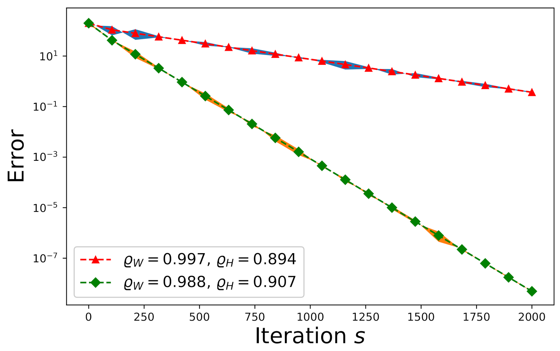
First consider a consistent system. The entries of $\mathbf{W}$, $\mathbf{H}$, and $\mathbf{c}$ are drawn from an independently and identically distributed (i.i.d.) random Gaussian process with zero-mean and unit variance where $m=200$, $n=150$, and $k=100$. We plot the convergence trends of the expected error $\mathbb{E}\left[{∥\mathbf{H}{\mathbf{y}}_t-\mathbf{H}{\mathbf{y}}_{opt}∥}_2^2\right]$ and the actual $L_2$-errors (shown by the shadow areas) with respect to $({\varrho }_{\mathbf{W}}=0.997,{\varrho }_{\mathbf{H}}=0.894)$ and $({\varrho }_{\mathbf{W}}=0.988,{\varrho }_{\mathbf{H}}=0.907)$ in Figure 4. The convergence speed subject to ${\varrho }_{\mathbf{W}}=0.997$ is slower than that subject to ${\varrho }_{\mathbf{W}}=0.988$ because the convergence speed is determined solely by ${\varrho }_{\mathbf{W}}$ according to Equation (26), where ${\varrho }_{\mathbf{H}}=\frac{{\varrho }_{\mathbf{W}}}{\zeta }$ and ${\varrho }_{\mathbf{W}}>{\varrho }_{\mathbf{H}}$. Each shadow region spans over the actual $L_2$-errors resulting from one hundred Monte Carlo trials.

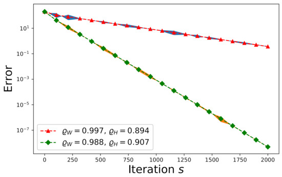
Figure 4. The effect of ${\varrho }_{\mathbf{W}}$ on the convergence of a random consistent system.

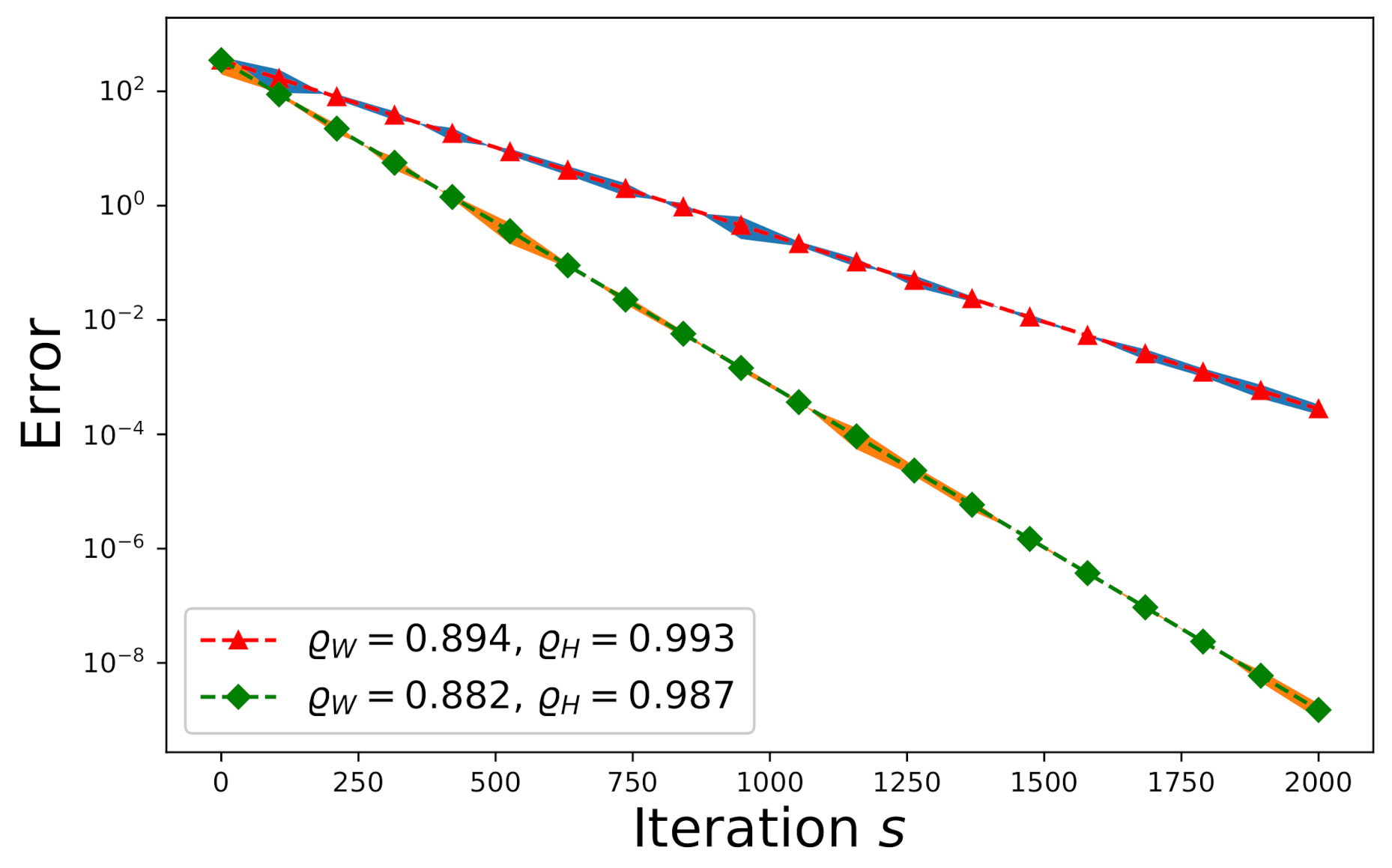
On the other hand, consider an inconsistent system. One has to apply Algorithm 2 to solve it. The entries of $\mathbf{W}$, $\mathbf{H}$, and $\mathbf{c}$ are drawn from an independently and identically distributed (i.i.d.) random Gaussian process with zero-mean and unit variance where $m=200$, $n=150$, and $k=100$. We plot the convergence trends of the expected error $\mathbb{E}\left[{∥\mathbf{H}{\mathbf{y}}_t-\mathbf{H}{\mathbf{y}}_{opt}∥}_2^2\right]$ and the actual $L_2$-errors (shown by the shadow areas) with respect to $({\varrho }_{\mathbf{W}}=0.894,{\varrho }_{\mathbf{H}}=0.993)$ and $({\varrho }_{\mathbf{W}}=0.882,{\varrho }_{\mathbf{H}}=0.987)$ in Figure 5. Again, the convergence speed subject to ${\varrho }_{\mathbf{H}}=0.993$ is slower than that subject to ${\varrho }_{\mathbf{H}}=0.987$ because the convergence speed is determined solely by ${\varrho }_{\mathbf{H}}$ according to Equation (32), where ${\varrho }_{\mathbf{H}}>{\varrho }_{\mathbf{W}}$. Each shadow region spans over the actual $L_2$-errors resulting from one hundred Monte Carlo trials.

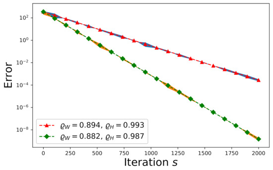
Figure 5. The effect of ${\varrho }_{\mathbf{H}}$ on the convergence of a random inconsistent system.

6.2. Validation Using Real-World Data

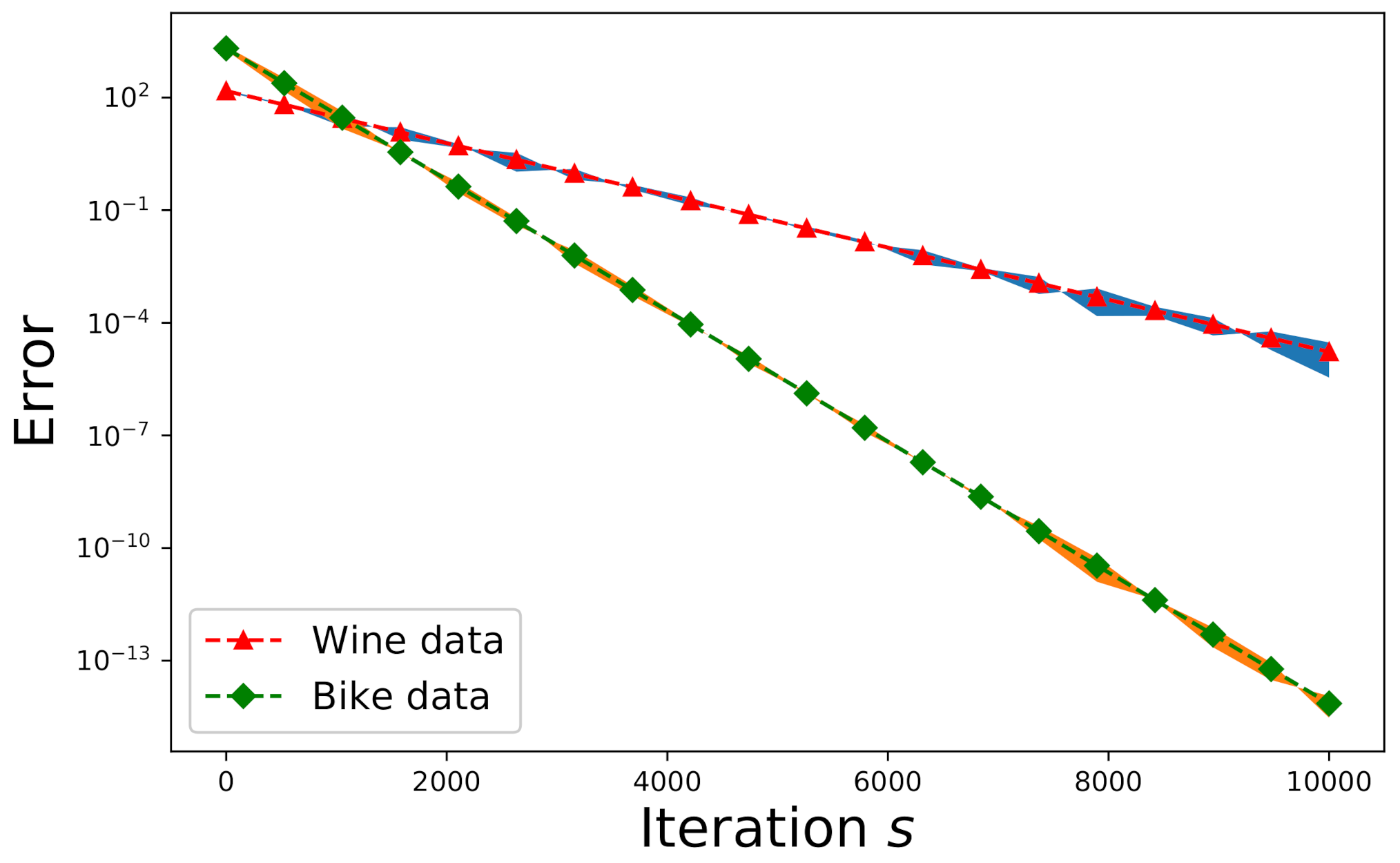
In addition to the Monte Carlo simulations shown in Section 6.1, we also validate our proposed new algorithms for real-world data on wine quality and bike rental. Here we use two real-world datasets from the UCI Machine Learning Repository [49]. The first set is related to wine quality, where we chose the data related to red wine only. The owner of this data set invoked twelve physicochemical and sensory variables to measure the wine quality. These variables include: 1—fixed acidity, 2—volatile acidity, 3—citric acid, 4—residual sugar, 5—chlorides, 6—free sulfur dioxide, 7—total sulfur dioxide, 8—density, 9—pH value, 10—sulphates, 11—alcohol, and 12—quality (each score ranging from 0 to 10). Consequently, these twelve categories of data can form an overdetermined matrix (as a matrix $\mathbf{V}$) with size $1599\times 12$. If the nonnegative matrix factorization is applied to obtain the factorized matrices $\mathbf{W}$ and $\mathbf{H}$ for $k=5$, we have ${\varrho }_{\mathbf{W}}=0.99840647$ and ${\varrho }_{\mathbf{H}}=0.99838774$. The expected errors $\mathbb{E}\left[{∥\mathbf{H}{\mathbf{y}}_t-\mathbf{H}{\mathbf{y}}_{opt}∥}_2^2\right]$ and the actual $L_2$ errors for wine data (denoted by triangle) are depicted in Figure 6, where Algorithm 2 is applied to solve the pertinent linear-regression problem in this case. On the other hand, another dataset about a bike-sharing system includes categorical and numerical data. Since the underlying problem is linear regression, we can work on the numerical attributes of the data only. These attributes include: 1—temperature, 2—feeling temperature, 3—humidity, 4—windspeed, 5—causal counts, 6—registered counts, and 7—total rental-bike counts. The matrix size for this dataset is thus $17,379\times 7$, and the corresponding parameters to this matrix are ${\varrho }_{\mathbf{W}}=0.99599172$, ${\varrho }_{\mathbf{H}}=0.98568833$, and $k=7$. The expected errors $\mathbb{E}\left[{∥\mathbf{H}{\mathbf{y}}_t-\mathbf{H}{\mathbf{y}}_{opt}∥}_2^2\right]$ and the actual $L_2$ errors for bike data (denoted by rhombus) are delineated in Figure 6.

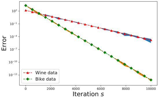
Figure 6. Error-convergence comparison for the wine data and the bike-rental data.

6.3. Time-Complexity Study

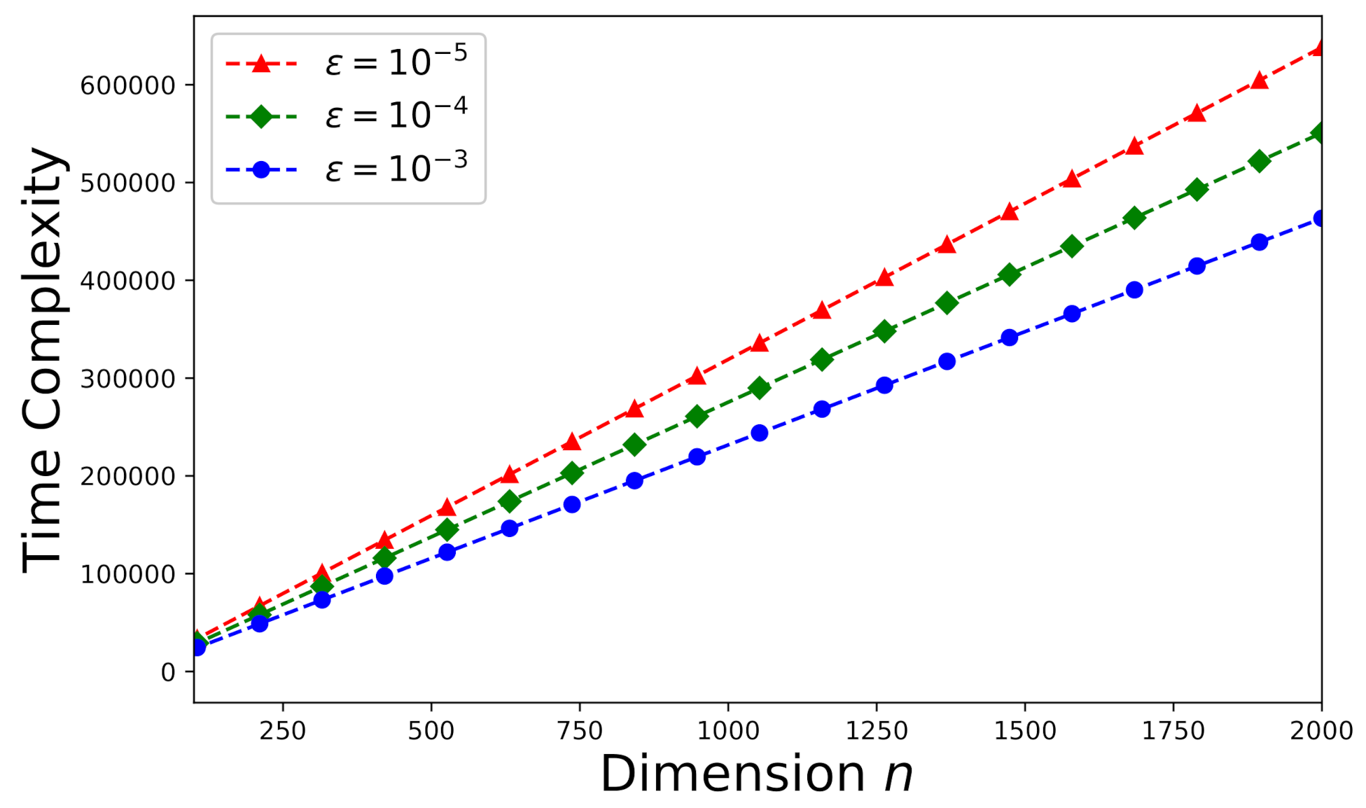
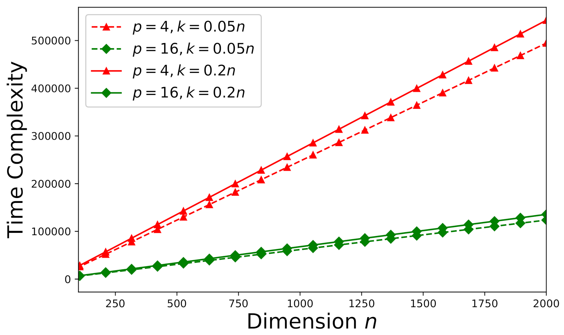
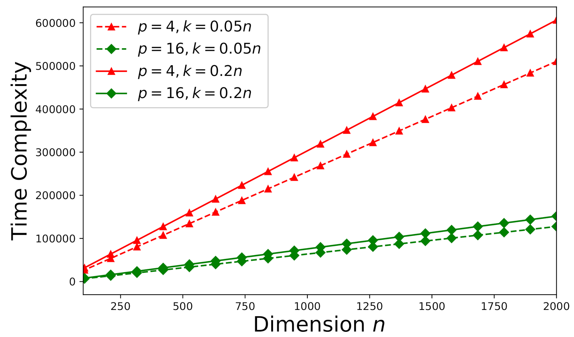
The time-complexity is studied here according to the theoretical analysis in Section 5.1. First consider an arbitrary consistent system (a random sample drawn from the Monte Carlo trials stated in Section 6.1). The effect of error tolerance $ϵ$ on time-complexity can be visualized in Figure 7. It can be observed that time-complexity increases as $ϵ$ decreases. In addition, we would like to investigate the effects of the number of processors p and the dimension k on time-complexity. The time-complexity results versus the number of processors p and the dimension k are presented in Figure 8 subject to $ϵ={10}^{-5}$.

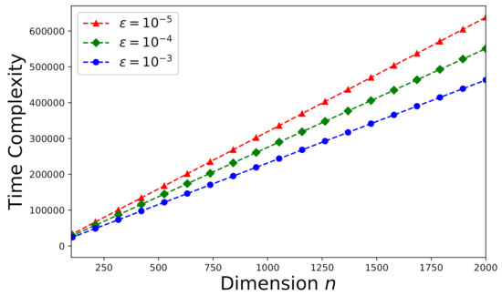
Figure 7. Time-complexity versus n for an arbitrary consistent system ($k=100$, $m=1.25n$).

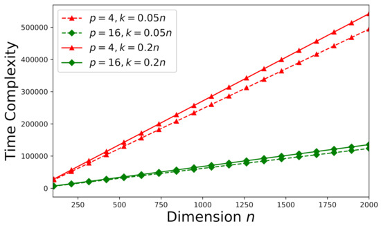
Figure 8. Time-complexity versus the number of processors p and the dimension k subject to $ϵ={10}^{-5}$ for an arbitrary consistent system ($m=1.25n$).

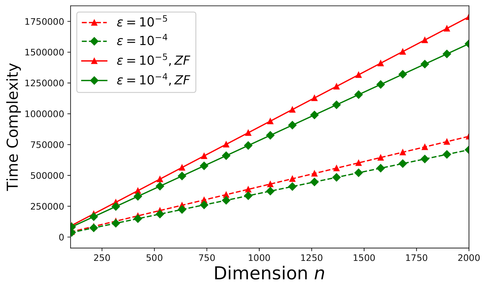
On the other hand, let’s focus on an arbitrary inconsistent system (an arbitrary Monte Carlo trial as stated in Section 6.1) now. The corresponding time-complexities for $ϵ={10}^{-5}$ and $ϵ={10}^{-4}$ are delineated by Figure 9. Note that one more vector is required to be updated in Algorithm 2 compared to Algorithm 1, the time-complexities shown in Figure 9 are higher that those shown in Figure 7 subject to the same $ϵ$. Because our derived error-estimate bound is tighter than that presented in [46] for the EGSA, the time-complexity of the proposed method for an inconsistent system has been reduced about 60% from that of the approach proposed by [46] subject to the same $ϵ$. How the number of processors p and the dimension k affect the time-complexity for inconsistent systems is illustrated by Figure 10 subject to the error tolerance $ϵ={10}^{-5}$.

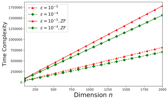
Figure 9. Time-complexity versus n for an arbitrary inconsistent system ($k=100$, $m=1.25n$). The curves denoted by “ZF” illustrate the theoretical time-complexity error-bounds for solving the original system involving the matrix $\mathbf{V}$ without factorization (theoretical results from [46]).

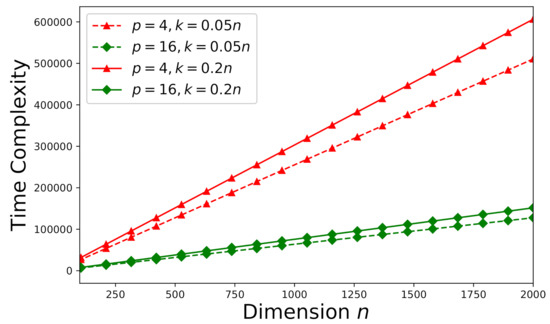
Figure 10. Time-complexity versus the number of processors p and the dimension k subject to $ϵ={10}^{-5}$ for an inconsistent system ($m=1.25n$).

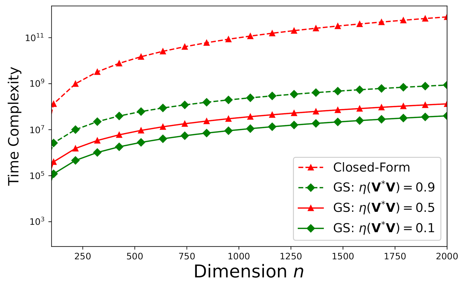
According to [50], we define the spectral radius $\eta \left(\mathbf{A}\right)$ of the “iteration matrix” $\mathbf{A}$$\stackrel{\mathrm{def}}{=}$${\mathbf{V}}^{\ast }\mathbf{V}$, where $\mathbf{V}$ is given by Equation (1), by:

$$\begin{array}{c}\hfill \eta \left(\mathbf{A}\right)\stackrel{\mathrm{def}}{=}max\left\{\left|{\lambda }_1\right|,\left|{\lambda }_2\right|,\cdots ,\left|{\lambda }_{\left|\mathbf{A}\right|}\right|\right\}.\end{array}$$

(48)

Note that $\left|\mathbf{A}\right|$ denotes the cardinality of $\mathbf{A}$ and ${\lambda }_1$, ${\lambda }_2$, …, ${\lambda }_{\left|\mathbf{A}\right|}$ specify the eigenvalues of $\mathbf{A}$. In Figure 11, we delineate the time-complexities required by the close-form solution (denoted by “Closed-Form” in the figure) and our proposed iterative Gauss–Seidel approach (denoted by “GS” in the figure) versus the dimension n for $\mathbf{V}$ with different spectral radii subject to $ϵ$ = ${10}^{-10}$ for an inconsistent system ($m=1.25n$) such that $\eta \left({\mathbf{V}}^{\ast }\mathbf{V}\right)$ = $0.9$, $0.5$, and $0.1$. Even under such a small error tolerance $ϵ$ = ${10}^{-10}$, the time-complexity required by the closed-form solution to Equation (1) is still much larger than the that required by the iterative Gauss–Seidel algorithm proposed in this work when only a single processor is used.

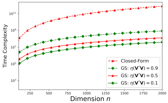
Figure 11. Time-complexity versus n for $\mathbf{V}$ with different spectral radii subject to $ϵ$=${10}^{-10}$ for an arbitrary inconsistent system ($m=1.25n$) such that $\eta \left({\mathbf{V}}^{\ast }\mathbf{V}\right)$ = $0.9$, $0.5$, and $0.1$.

Figure 11 demonstrates that if $\eta \left({\mathbf{V}}^{\ast }\mathbf{V}\right)$ < 1, our proposed new iterative Gauss–Seidel approach requires less time-complexity than the exact (closed-form) solution. According to Figure 11, the time-complexity advantage of our proposed approach becomes more significant as the dimension grows.

The run-time results listed by Table 1 and Table 2 are evaluated for different dimensions: k = $0.2n$ and m = $1.2n$ with respect to different n. The run-time unit is seconds. The computer specifications are as follows: GeForce RTX 3080 Laptop GPU, Windows 11 Home, 12th Gen Intel Core i9 processor, and SSD 8GB. Table 1 compares the run-times for the LU matrix factorization method in [51] and alternate least-squares (ALS) method in [52] with respect to different dimensions involved in the factorization step formulated by Equation (1). According to Table 1, the ALS method leads to a shorter run-time compared to the LU matrix factorization method. Table 2 compares the run times of the LAPACK solver [53], our proposed Gauss–Seidel algorithms with the factorization step formulated by Equation (1) (acronymed as “Fac. Inc.” in the tables), and our proposed Gauss–Seidel algorithms without the factorization step formulated by Equation (1) (acronymed as “Fac. Exc.” in the tables) for ${\varrho }_{max}$ = $0.99$ and ${\varrho }_{max}$ = $0.01$. If ${\varrho }_{max}$ = $0.99$, the convergence speeds of our proposed Gauss–Seidel algorithms are slow since ${\varrho }_{max}$ is close to one and thus it requires a longer time than the LAPACK solver. However, our proposed method can outperform the LAPACK solver when ${\varrho }_{max}$ is small since our proposed Gauss–Seidel algorithms will converge to the solution much faster.

Table 1. Run-times (in seconds) for the factorization of $\mathbf{V}$.

Dimensions, n	100	1000	10,000	100,000
LU	5.31	8.18 × 10${}^1$	2.18 × 10${}^2$	7.01 × 10${}^3$
ALS	4.31	17.81	9.18 × 10${}^1$	4.81 × 10${}^2$

Table 2. Run-times (in seconds) for solving $\mathbf{V}$ using the Gauss–Seidel algorithms.

Dimensions, n	100	1000	10,000	100,000
${\varrho }_{max}$ = $0.99$, LAPACK	5.71	25.1	2.4 × 10${}^2$	9.2× 10${}^2$
${\varrho }_{max}$ = $0.99$, Fac. Inc.	6.63	41.61	8.08 × 10${}^2$	2.30 × 10${}^3$
${\varrho }_{max}$ = $0.99$, Fac. Exc.	2.32	23.8	7.18 × 10${}^2$	1.91 × 10${}^3$
${\varrho }_{max}$ = $0.01$, LAPACK	5.31	23.1	2.28 × 10${}^2$	9.01 × 10${}^2$
${\varrho }_{max}$ = $0.01$, Fac. Inc.	4.43	20.1	1.71 × 10${}^2$	7.60 × 10${}^2$
${\varrho }_{max}$ = $0.01$, Fac. Exc.	0.13	2.31	8.18 × 10${}^1$	2.81 × 10${}^2$

6.4. Memory-Complexity Study

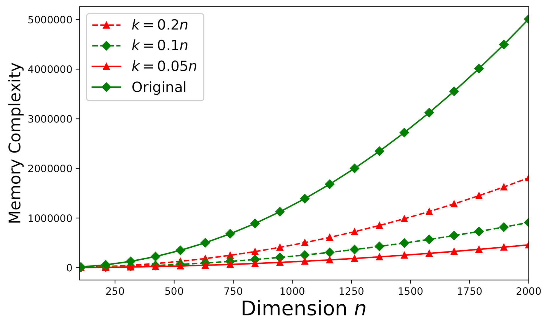
Memory-complexity is also investigated here according to the theoretical analysis stated in Section 5.2. Figure 12 depicts the required memory-complexity for solving an arbitrary consistent system (the same as the system used in Section 6.3) using Algorithm 1. The memory-complexity is evaluated for different dimensions: $k=0.2n$, $k=0.1n$, and $k=0.05n$. We further set $m=1.25n$. On the other hand, for an arbitrary inconsistent system (the same as the system used in Section 6.3), all of the aforementioned values of m, n, and k remain the same and Algorithm 2 should be applied instead. Figure 13 plots the required memory-complexity for solving an inconsistent system using Algorithm 2. In Figure 12 and Figure 13, for both consistent and inconsistent systems, we also present the required memory-complexity for solving the original system involving the matrix $\mathbf{V}$ without factorization. According to Figure 12 and Figure 13, the storage-efficiency can be significantly improved by at least 75% to 90% (dependent on the dimension k).

Figure 12. The memory -complexity versus n for a consistent system ($m=1.25n$).

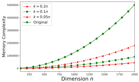
Figure 13. The memory -complexity versus n for an inconsistent system ($m=1.25n$).

7. Conclusions

For a wide variety of big-data analytics applications, we designed two new efficient parallel algorithms, which are built upon the Gauss–Seidel algorithm, to solve large linear-regression problems for both consistent and inconsistent systems. This new approach can save computational resources by transforming the original problem into subproblems involving factorized matrices of much smaller dimensions. Meanwhile, the theoretical expected-error estimates were derived to study the convergences of the new algorithms for both consistent and inconsistent systems. Two crucial computational resource metrics—time-complexity and memory-complexity—were evaluated for the proposed new algorithms. Numerical results from artificial simulations and real-world data demonstrated the convergence and the efficiency (in terms of computational resource usage) of the proposed new algorithms. Our proposed new approach is much more efficient in both time and memory than the conventional method. Since the prevalent big-data applications frequently involve linear-regression problems (such as how to undertake linear regression when the associated matrix dimension is very large) with tremendous dimensions, our proposed new algorithms can be deemed very impactful and convenient to future big-data computing technology. In the future, we would like to consider the problem about how to perform the matrix factorization $\mathbf{V}$ properly to have ${\varrho }_{max}$ = $max({\varrho }_{\mathbf{W}},{\varrho }_{\mathbf{H}})$ as small as possible. If we have a smaller ${\varrho }_{max}$, we can expect faster convergences of our proposed Gauss–Seidel algorithms. In general, it is not always possible to have the linear system characterized by $\mathbf{V}$ having a small value of ${\varrho }_{max}$. Future research suggested here will help us to overcome this main challenge.

References

- Thakur, N.; Han, C.Y. An ambient intelligence-based human behavior monitoring framework for ubiquitous environments. Information 2021, 12, 81. [Google Scholar] [CrossRef]
- Chen, Y.; Ho, P.H.; Wen, H.; Chang, S.Y.; Real, S. On Physical-Layer Authentication via Online Transfer Learning. IEEE Internet Things J. 2021, 9, 1374–1385. [Google Scholar] [CrossRef]
- Tariq, F.; Khandaker, M.; Wong, K.-K.; Imran, M.; Bennis, M.; Debbah, M. A speculative study on 6G. arXiv 2019, arXiv:1902.06700. [Google Scholar] [CrossRef]
- Gu, R.; Tang, Y.; Tian, C.; Zhou, H.; Li, G.; Zheng, X.; Huang, Y. Improving execution concurrency of large-scale matrix multiplication on distributed data-parallel platforms. IEEE Trans. Parallel Distrib. Syst. 2017, 28, 2539–2552. [Google Scholar] [CrossRef]
- Dass, J.; Sarin, V.; Mahapatra, R.N. Fast and communication-efficient algorithm for distributed support vector machine training. IEEE Trans. Parallel Distrib. Syst. 2018, 30, 1065–1076. [Google Scholar] [CrossRef]
- Yu, Z.; Xiong, W.; Eeckhout, L.; Bei, Z.; Mendelson, A.; Xu, C. MIA: Metric importance analysis for big data workload characterization. IEEE Trans. Parallel Distrib. Syst. 2017, 29, 1371–1384. [Google Scholar] [CrossRef]
- Zhang, T.; Liu, X.-Y.; Wang, X.; Walid, A. cuTensor-Tubal: Efficient primitives for tubal-rank tensor learning operations on GPUs. IEEE Trans. Parallel Distrib. Syst. 2019, 31, 595–610. [Google Scholar] [CrossRef]
- Zhang, T.; Liu, X.-Y.; Wang, X. High performance GPU tensor completion with tubal-sampling pattern. IEEE Trans. Parallel Distrib. Syst. 2020, 31, 1724–1739. [Google Scholar] [CrossRef]
- Hu, Z.; Li, B.; Luo, J. Time-and cost-efficient task scheduling across geo-distributed data centers. IEEE Trans. Parallel Distrib. Syst. 2017, 29, 705–718. [Google Scholar] [CrossRef]
- Jaulmes, L.; Moreto, M.; Ayguade, E.; Labarta, J.; Valero, M.; Casas, M. Asynchronous and exact forward recovery for detected errors in iterative solvers. IEEE Trans. Parallel Distrib. Syst. 2018, 29, 1961–1974. [Google Scholar] [CrossRef] [Green Version]
- Chen, Y.; Wu, J.; Lin, J.; Liu, R.; Zhang, H.; Ye, Z. Affinity regularized non-negative matrix factorization for lifelong topic modeling. IEEE Trans. Knowl. Data Eng. 2019, 32, 1249–1262. [Google Scholar] [CrossRef]
- Kannan, R.; Ballard, G.; Park, H. MPI-FAUN: An MPI-based framework for alternating-updating nonnegative matrix factorization. IEEE Trans. Knowl. Data Eng. 2017, 30, 544–558. [Google Scholar] [CrossRef]
- Wang, S.; Chen, H.; Cao, J.; Zhang, J.; Yu, P. Locally balanced inductive matrix completion for demand-supply inference in stationless bike-sharing systems. IEEE Trans. Knowl. Data Eng. 2019, 32, 2374–2388. [Google Scholar] [CrossRef]
- Sharma, S.; Powers, J.; Chen, K. PrivateGraph: Privacy-preserving spectral analysis of encrypted graphs in the cloud. IEEE Trans. Knowl. Data Eng. 2018, 31, 981–995. [Google Scholar] [CrossRef]
- Liu, Z.; Vandenberghe, L. Interior-point method for nuclear norm approximation with application to system identification. SIAM J. Matrix Anal. Appl. 2009, 31, 1235–1256. [Google Scholar] [CrossRef]
- Borg, I.; Groenen, P. Modern multidimensional scaling: Theory and applications. J. Educ. Meas. 2003, 40, 277–280. [Google Scholar] [CrossRef]
- Biswas, P.; Lian, T.-C.; Wang, T.-C.; Ye, Y. Semidefinite programming based algorithms for sensor network localization. ACM Trans. Sens. Netw. 2006, 2, 188–220. [Google Scholar] [CrossRef]
- Yan, K.; Wu, H.-C.; Xiao, H.; Zhang, X. Novel robust band-limited signal detection approach using graphs. IEEE Commun. Lett. 2017, 21, 20–23. [Google Scholar] [CrossRef]
- Yan, K.; Yu, B.; Wu, H.-C.; Zhang, X. Robust target detection within sea clutter based on graphs. IEEE Trans. Geosci. Remote Sens. 2019, 57, 7093–7103. [Google Scholar] [CrossRef]
- Costa, J.A.; Hero, A.O. Geodesic entropic graphs for dimension and entropy estimation in manifold learning. IEEE Trans. Signal Process. 2004, 52, 2210–2221. [Google Scholar] [CrossRef] [Green Version]
- Sandryhaila, A.; Moura, J.M. Big data analysis with signal processing on graphs. IEEE Signal Process. Mag. 2014, 31, 80–90. [Google Scholar] [CrossRef]
- Sandryhaila, A.; Moura, J.M. Discrete signal processing on graphs. IEEE Trans. Signal Process. 2013, 61, 1644–1656. [Google Scholar] [CrossRef] [Green Version]
- Ahmed, A.; Romberg, J. Compressive multiplexing of correlated signals. IEEE Trans. Inf. Theory 2014, 61, 479–498. [Google Scholar] [CrossRef] [Green Version]
- Davies, M.E.; Eldar, Y.C. Rank awareness in joint sparse recovery. IEEE Trans. Inf. Theory 2012, 58, 1135–1146. [Google Scholar] [CrossRef] [Green Version]
- Cong, Y.; Liu, J.; Fan, B.; Zeng, P.; Yu, H.; Luo, J. Online similarity learning for big data with overfitting. IEEE Trans. Big Data 2017, 4, 78–89. [Google Scholar] [CrossRef]
- Zhu, X.; Suk, H.-I.; Huang, H.; Shen, D. Low-rank graph-regularized structured sparse regression for identifying genetic biomarkers. IEEE Trans. Big Data 2017, 3, 405–414. [Google Scholar] [CrossRef] [Green Version]
- Liu, X.-Y.; Wang, X. LS-decomposition for robust recovery of sensory big data. IEEE Trans. Big Data 2017, 4, 542–555. [Google Scholar] [CrossRef]
- Fan, J.; Zhao, M.; Chow, T.W.S. Matrix completion via sparse factorization solved by accelerated proximal alternating linearized minimization. IEEE Trans. Big Data 2018, 6, 119–130. [Google Scholar] [CrossRef]
- Hou, D.; Cong, Y.; Sun, G.; Dong, J.; Li, J.; Li, K. Fast multi-view outlier detection via deep encoder. IEEE Trans. Big Data 2020, 1–11. [Google Scholar] [CrossRef]
- Hotelling, H. Analysis of a complex of statistical variables into principal components. J. Educ. Psychol. 1933, 24, 417–441. [Google Scholar] [CrossRef]
- Landauer, T.K.; Foltz, P.W.; Laham, D. An introduction to latent semantic analysis. Discourse Process. 1998, 25, 259–284. [Google Scholar] [CrossRef]
- Obozinski, G.; Taskar, B.; Jordan, M.I. Joint covariate selection and joint subspace selection for multiple classification problems. Stat. Comput. 2010, 20, 231–252. [Google Scholar] [CrossRef] [Green Version]
- Liu, H.; Wu, J.; Liu, T.; Tao, D.; Fu, Y. Spectral ensemble clustering via weighted k-means: Theoretical and practical evidence. IEEE Trans. Knowl. Data Eng. 2017, 29, 1129–1143. [Google Scholar] [CrossRef]
- Jiang, X.; Zeng, W.-J.; So, H.C.; Zoubir, A.M.; Kirubarajan, T. Beamforming via nonconvex linear regression. IEEE Trans. Signal Process. 2015, 64, 1714–1728. [Google Scholar] [CrossRef]
- Kallummil, S.; Kalyani, S. High SNR consistent linear model order selection and subset selection. IEEE Trans. Signal Process. 2016, 64, 4307–4322. [Google Scholar] [CrossRef]
- Kallummil, S.; Kalyani, S. Residual ratio thresholding for linear model order selection. IEEE Trans. Signal Process. 2018, 67, 838–853. [Google Scholar] [CrossRef]
- So, H.C.; Zeng, W.-J. Outlier-robust matrix completion via lp-minimization. IEEE Trans. Signal Process. 2018, 66, 1125–1140. [Google Scholar]
- Berberidis, D.; Kekatos, V.; Giannakis, G.B. Online censoring for large-scale regressions with application to streaming big data. IEEE Trans. Signal Process. 2016, 64, 3854–3867. [Google Scholar] [CrossRef] [Green Version]
- Boloix-Tortosa, R.; Murillo-Fuentes, J.J.; Tsaftaris, S.A. The generalized complex kernel least-mean-square algorithm. IEEE Trans. Signal Process. 2019, 67, 5213–5222. [Google Scholar] [CrossRef]
- Widrow, B. Adaptive Signal Processing; Prentice Hall: Hoboken, NJ, USA, 1985. [Google Scholar]
- Sonneveld, P.; Van Gijzen, M.B. IDR (s): A family of simple and fast algorithms for solving large nonsymmetric systems of linear equations. SIAM J. Sci. Comput. 2009, 31, 1035–1062. [Google Scholar] [CrossRef] [Green Version]
- Bavier, E.; Hoemmen, M.; Rajamanickam, S.; Thornquist, H. Amesos2 and Belos: Direct and iterative solvers for large sparse linear systems. Sci. Program. 2012, 20, 241–255. [Google Scholar] [CrossRef] [Green Version]
- Chang, S.Y.; Wu, H.-C. Divide-and-Iterate approach to big data systems. IEEE Trans. Serv. Comput. 2020. [Google Scholar] [CrossRef]
- Hageman, L.; Young, D. Applied Iterative Methods; Academic Press: Cambridge, MA, USA, 1981. [Google Scholar]
- Leventhal, D.; Lewis, A.S. Randomized methods for linear constraints: Convergence rates and conditioning. Math. Oper. Res. 2010, 35, 641–654. [Google Scholar] [CrossRef] [Green Version]
- Ma, A.; Needell, D.; Ramdas, A. Convergence properties of the randomized extended Gauss–Seidel and Kaczmarz methods. SIAM J. Matrix Anal. Appl. 2015, 36, 1590–1604. [Google Scholar] [CrossRef] [Green Version]
- Weiss, N.A. A Course in Probability; Addison-Wesley: Boston, MA, USA, 2006. [Google Scholar]
- Harremoës, P. Bounds on tail probabilities in exponential families. arXiv 2016, arXiv:1601.05179. [Google Scholar]
- Dua, D.; Graff, C. UCI Machine Learning Repository. 2017. Available online: http://archive.ics.uci.edu/ml (accessed on 3 March 2022).
- Li, C.-K.; Tam, T.-Y.; Tsing, N.-K. The generalized spectral radius, numerical radius and spectral norm. Linear Multilinear Algebra 1984, 16, 215–237. [Google Scholar] [CrossRef]
- Mittal, R.; Al-Kurdi, A. LU-decomposition and numerical structure for solving large sparse nonsymmetric linear systems. Comput. Math. Appl. 2002, 43, 131–155. [Google Scholar] [CrossRef] [Green Version]
- Kroonenberg, P.M.; De Leeuw, J. Principal component analysis of three-mode data by means of alternating least squares algorithms. Psychometrika 1980, 45, 69–97. [Google Scholar] [CrossRef]
- Kågström, B.; Poromaa, P. LAPACK-style algorithms and software for solving the generalized Sylvester equation and estimating the separation between regular matrix pairs. ACM Trans. Math. Softw. 1996, 22, 78–103. [Google Scholar] [CrossRef]
Publisher’s Note: MDPI stays neutral with regard to jurisdictional claims in published maps and institutional affiliations. |
© 2022 by the authors. Licensee MDPI, Basel, Switzerland. This article is an open access article distributed under the terms and conditions of the Creative Commons Attribution (CC BY) license (https://creativecommons.org/licenses/by/4.0/).