Generalized Differentiability of Continuous Functions


1
Environment, Health and Safety, IMEC vzw, Kapeldreef 75, 3001 Leuven, Belgium
2
MMSDP, IICT, Bulgarian Academy of Sciences, Acad. G. Bonchev St., Block 25A, 1113 Sofia, Bulgaria
Fractal Fract. 2020, 4(4), 56; https://doi.org/10.3390/fractalfract4040056
Submission received: 19 October 2020
/
Revised: 2 December 2020
/
Accepted: 3 December 2020
/
Published: 10 December 2020
(This article belongs to the Special Issue New Aspects of Local Fractional Calculus)
Abstract
:Many physical phenomena give rise to mathematical models in terms of fractal, non-differentiable functions. The paper introduces a broad generalization of the derivative in terms of the maximal modulus of continuity of the primitive function. These derivatives are called indicial derivatives. As an application, the indicial derivatives are used to characterize the nowhere monotonous functions. Furthermore, the non-differentiability set of such derivatives is proven to be of measure zero. As a second application, the indicial derivative is used in the proof of the Lebesgue differentiation theorem. Finally, the connection with the fractional velocities is demonstrated.
Keywords:
fractals; Smith–Volterra–Cantor set; Cantor functions; differentiable functions; Lipschitz (Hölder) classesMSC:
26A30; 26A161. Introduction
From a certain perspective, a derivative can be interpreted as an idealization of the linear approximation. Moreover, the derivatives are indispensable tools for physical modelling. In classical physics, the second law of Newton tacitly assumes that the velocity is a differentiable function of time. This ensures mathematical modelling in terms of differential equations, and hence (almost everywhere) differentiable functions. Ampere even tried to prove that all functions are almost everywhere differentiable [1]. Now we know that this attempt was doomed to fail. Various non-differentiable functions were constructed in the 19th century and regarded with a mixture of wonder and horror (historical survey in [2]). For example, Charles Hermite wrote “I turn with terror and horror from this lamentable scourge of functions with no derivatives”, while Henri Poincaré denounced these functions as “an outrage against common sense”. The interest in fractal and non-differentiable functions was rekindled with the works of Mandelbrot in fractals [3]. Moreover, many physical phenomena give rise to models in terms of fractal, non-differentiable functions. Such an opposition leads to the question whether the ordinary (i.e., Cauchy) derivatives can be generalized locally in a way that can describe such irregular objects. This is certainly achievable for a class of singular functions, such as the De Rham’s function, which can be characterized locally in terms of fractional velocity [4,5]. Purely mathematically, the derivatives can be generalized in several ways. Derivatives can be defined in the usual way as limits of difference quotients on the accumulation sets of points [6], (Chaper 3, p. 105). This approach can be applied also to functions defined on perfect fractal sets as demonstrated in [7,8,9].
Having physical applications in mind, it is logical to restrict the functions of study to continuous ones. Such functions will be allowed to vary everywhere on the real line. So this condition makes the setting very different from the approach of Pravate, Gangal and Yang.
A very broad generalization of derivatives can be achieved if the linear, Lipschitz, growth condition is replaced by a non-linear one. From this perspective, the growth condition can be taken as the modulus of continuity. Such notion is by necessity limited. However, it provides a framework which allows one to identify if a certain property of derivatives carries over to more particular constructs, for example in the setting of fractional velocities [10], or it is special for the linear growth condition.
The paper is organized as follows. Section 2 introduces some general definitions and notations. Section 3 introduces the oscillation of functions. Section 4 introduces indicial derivatives. Section 5 gives the construction of a singular function used to clarify the Lebesgue differentiation theorem. Section 6 characterizes the continuity sets of derivatives. Section 7 characterizes the fractional velocities in terms of the indicator derivatives.
2. General Definitions and Conventions
The term variable denotes an indefinite number taken from a predefined set, usually the real numbers. Sets are denoted by capital letters, while variables taking values in sets are denoted by lowercase. The term function denotes a mapping from one number to another and the action of the function is denoted as . Implicitly the mapping acts on the real numbers: . If a statement of a function f fulfils a certain predicate with argument A (i.e., ) the following short-hand notation will be used .
The co-domain of the function is denoted as . The term operator denotes the mapping from a functional expression to functional expression. The term functional denotes the mapping from a functional expression to a number. Square brackets are used for the arguments of operators and functionals, while round brackets are used for the arguments of functions. The term Cauchy sequence will always be interpreted as a null sequence.
Everywhere, will be considered as a small positive variable. The asymptotic small notation will be used as introduced in [5].
Definition 1.
Define the parametrized difference operators acting on the function as
for the variable . The two operators are referred to as forward difference and backward difference operators, respectively.
Definition 2
(Anonymous function notation). The notation for the pair will be interpreted as the implication that if Left-Hand Side (LHS) is fixed then the Right-Hand Side (RHS) is fixed by the value chosen on the left, i.e., as an anonymous functional dependency .
3. The Discontinuity Sets of Functions
In order to state the main result of the section we introduce the auxiliary concept of function oscillation.
Definition 3
(Oscillation). Define the oscillation of the function f in the interval as
Definition 4
(Directed Oscillation). Define the directed oscillations as (i) the forward oscillation:
and the backward oscillation:
The lemma was stated in [11]:
Lemma 1
(Oscillation lemma). Consider the function . Suppose that , , respectively.
If then f is right-continuous at x. Conversely, if f is right-continuous at x then . If then f is left-continuous at x. Conversely, if f is left-continuous at x then . That is,
Then the negation of the statement is also true.
Corollary 1.
The following two statements are equivalent
Theorem 1
(Disconnected discontinuity set). Consider a bounded function F defined on the compact interval I. Then its set of discontinuity is totally disconnected in I.
Proof.
Consider a decreasing collection of closed nested intervals from a partition of the interval (, not necessarily small); that is , .
Since the case when the function is locally constant is trivial we consider only two cases: increasing and decreasing. Let and define
Increasing case: Suppose that F is increasing in then
Decreasing case: Suppose that F is decreasing in then
On the other hand, and . If F is continuous on the opening of , in limit
and . On the other hand, F can be discontinuous on the boundary points , which are disconnected.
Suppose then that both endpoints are points of discontinuity. Hence, . If F is discontinuous on the opening of , we take and proceed in the same way. Therefore, is a union of totally disconnected sets and hence it is totally disconnected. □
The disconnected discontinuity theorem is used as the main tool characterizing the continuity sets of derivatives.
4. Indicial Derivatives
Definition 5
(Modulus of continuity). A modulus of continuity is a
- (1)
- non-decreasing continuous function, such that
- (2)
- and
- (3)
- holds in the interval for some constant .
I is assumed to be in the domain of the function f. In addition, a regular modulus will be such that .
Definition 6.
Consider a bounded function f defined on a compact interval I. Define the right (resp. left) point oscillation functions as
This section introduces the indicator or -derivatives. I propose this name based on the properties of their image sets. These derivative behave in a way like the signed indicator function of a set.
Definition 7.
Define the right and left modulus-variation operators as
for a positive ϵ.
Definition 8.
For a function f define superior and inferior, and respectively forward and backward, Dini-type ω derivatives, as the limit numbers L
for all , .
Remark 1.
These derivative functions obviously generalize the concept of Dini derivatives:
for the function f. It can be seen also that all four such -derivatives are of Baire I class (Definition A3).
Equipped with the above definition we can state the first existence result:
Theorem 2
(Bounded -derivatives). For a continuous function the four derivative functions exist as real numbers. Moreover, if f is non-decreasing about
while if f is non-increasing about
Proof.
Let be given and x is fixed but we can vary . Consider the auxiliary function
The supremum definitions are restatements of the Least Upper Bound (LUB) property for in terms of the variable , while the infimum derivatives are restatements with the Greatest Lower Bound (GLB) property of the reals again for the same variable. Therefore, all four numbers exist for a given argument x and, therefore, under the above hypothesis. Moreover, since then for an non-decreasing function . Therefore, by the supremum property . For a decreasing function f it is sufficient to consider and apply the same arguments. □
We can give generalized definition of local differentiability (called -differentiability) as follows:
Definition 9.
A function f is ω-differentiable at x if at least one of the two limits exist
where the conventions for and ϵ are as in Definition 8.
Note that the definition only supposes that the one-sided limits of the increments— (respectively ) exist as real numbers. That is,
is admissible. This is the minimal statement that can be given for the limit of an increment of a function. Nevertheless, based on two strong properties—monotonicity and continuity—it can be claimed that
Theorem 3
(Monotone -differentiation). If a function f is monotone and continuous in a compact interval I then it is continuously ω-differentiable everywhere in the opening . If f is increasing in then . If f is decreasing in then . If f is increasing in then . If f is decreasing in then .
Proof.
The continuity follows directly from Theorem 3, while the restriction comes from the fact that at the boundary only one of the increments can be defined without further hypothesis for the values of f outside of I. The evaluation of the derivatives comes as follows. Fix x and consider . The proof follows from the fact that in both cases . □
Definition 10.
Functions of the bounded variation (see Definition A1) on a compact interval I will be denoted by . If further the function is continuous on I it will be denoted by .
Theorem 4
(BVC -differentiation). If the function f is in a closed interval I then it is ω-differentiable everywhere in the opening .
Proof.
The proof follows from the Jordan theorem, since a BV[I] function can be decomposed into a difference of two non-decreasing functions. On the other hand, without further hypotheses we can not claim anything about the eventual equality of and since so that we can form only the trivial map , which without further restrictions of the domain of x (i.e., by means of some topological obstructions) is uncountable. □
We can further utilize the concept of oscillation to give a concise general differentiability condition as
Theorem 5
(Characterization of -derivative). The following implications hold
so that if Equation (4) holds at x then f is ω-differentiable (and hence continuous) at x.
Proof.
Continuity implication Consider the inequality
so that
Let and . Then by the triangle inequality
Therefore, in limit , hence and f is continuous. This sequence of operations reminds the fact that real numbers are constructed by a limiting process.
Forward statement: Suppose that and Then by LUB
so that
Then by the triangle inequality
Then in limit, by Lemma 1
Further, starting from
Therefore,
Therefore, all three limits coincide.
Converse statement: Suppose that
By hypothesis
Therefore, in limit
so that . □
Corollary 2
(Range of ). The range of is given by the discrete set
Proof.
Let be given. If f is constant in I trivially . If f is increasing in I then and by duality if f is decreasing in I then . □
The non-differentiability set of a continuous function can be characterized by the following theorem.
Theorem 6
( non-differentiability set). Consider the function on the compact interval I. Then the sets
are null sets. That is, for a continuous function the ω non-differentiability set is null (see Definition A2).
Proof.
Consider the case wherever the right -derivative does not exist. That is, the defining quotient oscillates without a limit. Then for
for some . We can consider a variable . There is a rational . Associate so that can be counted by an enumeration of the rationals and index . Therefore, the set
is countable . Since is totally disconnected by Theorem 1 we can choose and . Therefore,
so that is a null set by Definition A2. The left case holds by duality. □
5. Fat Cantor Sets and Related Quasi-Singular Functions
There are sets that are totally disconnected, uncountable and non-null. An example of such sets is the Smith–Volterra–Cantor set (i.e., the so-called Fat Cantor set), which is of measure . The construction of the Smith–Volterra–Cantor set is given as follows: The set is constructed by iteratively removing certain intervals from the unit interval . At each step k, the length that is removed from the middle of each of the remaining intervals. That is, starting from and on every step
That is .
For example,
During the process, disjoint intervals of total length
are removed so that the resulting set is of measure . The Smith–Volterra–Cantor set is closed as it is an intersection of closed sets. Furthermore, at step n the length of each closed subinterval is . Starting from one gets
Therefore, by the Nested Interval Theorem the Smith–Volterra–Cantor (SVC) set is totally disconnected and contains no intervals. The set presented above can be used to construct a quasi-singular function, called Smith–Volterra–Cantor (SVC) function. The quasi-singularity will be defined as the property of the function to have a totally disconnected set of change . Formally,
Definition 11
(Quasi-singular function). Denote the set by . A continuous function f is called quasi-singular on a compact interval I if
- f is non-constant on I.
- the complement is totally disconnected.
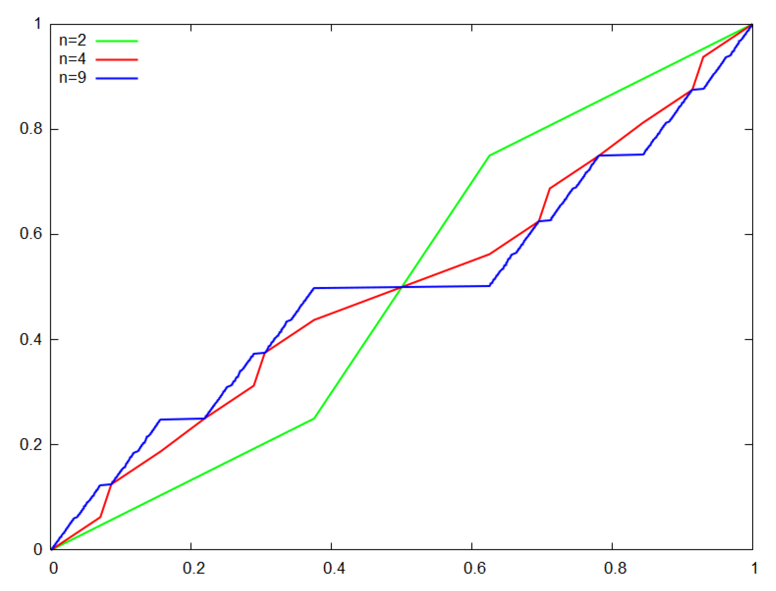
The appearance of the function is jagged and its general outline resembles the Cantor’s “Devil’s staircase” (see Figure 1). The function was introduced in [12].
Definition 12
(SVC Function). Define the SVC function as the continuous map between the SVC set defined above and the dyadic rationals in the following construction. Let be the sequence of the end-points of the interval in the n-th step in the construction of the SVC set. Let be the sequence of dyadic rationals with denominator excluding .
Define the sequence of continuous piece-wise linear interpolating functions (see Figure 1) , such that
and pass to the limit .
In contrast to the Cantor-Lebesgue function, the SVC function is Lipschitz on its set of change. In the following argument we characterize the set of growth of the SVC function. Let .
In the case of the SVC function . Then by construction, the set has measure . On the other hand, for and
Then by induction
Therefore, in limit
Then for the difference quotient
Therefore, in limit
while . Therefore, .
Theorem 7.
Let S denote the SVC set and . Then on and on . Moreover, .
Corollary 3.
The SVC function is quasi-singular.
The presented theorem has an impact on the formulation of the Lebesgue monotone differentiation theorem. In fact, it requires that the hypothesis of Lebesgue monotone differentiation theorem require strict monotonicity of the function. This refinement is done in the following section.
6. Continuity Sets of Derivatives
This section re-states the classical result of the Lebesgue differentiation theorem. The poof is given using the machinery of -differentiation. In the following argument I reserve the term “strictly monotone function” to mean only a strictly increasing or strictly decreasing function in an interval.
Theorem 8
(Lebesgue monotone differentiation theorem). Suppose that f is strictly monotone and continuous in the compact interval I. Then f is continuously differentiable almost everywhere. The set
is a null (see Definition A2).
Proof.
Let . Since f is strictly monotone and continuous then its -derivative exists by Theorem 3. Therefore, let . By Theorem 3 for
Therefore, by monotonicity using the original notation
hence and . The argument above is not applicable to the boundary points , however they are countable, since they can be covered by intervals with rational end-points, and hence the union of all B sets is a null set. □
Recall the definitions of nowhere monotone functions:
Definition 13.
A function is nowhere monotone in the compact interval , written NM[I], if given any
so that NM[I] function is neither non-decreasing nor non-increasing on any sub-interval of I. A function, which is nowhere monotone at a point (NM[y]), is treated as above while y is held fixed.
From the Lebesgue monotone differentiation theorem it follows that a nowhere differentiable function on an open interval I is simultaneously nowhere monotone on I. Brown et al. establish that no continuous function of bounded variation BVC is MN[y] [13] (Theorem 12. Corr. 3). That is to say for as above. Therefore, it is of interest to establish the following result.
Theorem 9
(NM continuous -differentiability). Suppose that and . Then
Proof.
Suppose that exists. The set is totally disconnected. This can be proven by contradiction. Suppose that the set M is connected hence, is continuous; and independently f is increasing in . However, . Therefore, in the limit
However, this a contradiction since f was supposed to be increasing in , hence M can not be connected.
By duality, the set is also totally disconnected. Hence, only the set must have connected components. □
The same conclusion is true if we replace the indicial derivative with the supremum Dini-type derivative
Corollary 4.
Suppose that and . Then
Theorem 10
(Continuity sets of derivatives). Consider a continuous function f on a compact interval I. Suppose that and are separately continuous wherever they exist then the following holds:
- (1)
- (2)
- is totally disconnected with empty interior.
- (3)
- The total discontinuity set can be written as , where is and is a null set.
- (4)
- The continuity set is . and are given by Definition A4
Proof.
Consider the interval . Then there is rational .
Associate so that can be counted by an enumeration of the rationals.
Assume that and are separately continuous on the opening of . Fix x, such that .
By continuity
However, since x and hence is arbitrary must hold . Hence, is continuous on .
By this argument we establish that the set is , where we also assume that whenever does not exist it is replaced by a value that makes discontinuous. By Theorem 1 the discontinuity set is totally disconnected and with empty interior.
Let us further consider the case wherever left and right derivatives do not exist (either diverge or oscillate without a limit). It is enough to consider the right derivative. Then we have that for
for some . We can consider a variable . There is a rational . Associate so that can be counted by an enumeration of the rationals and index . Therefore, the set
is countable . Since it is totally disconnected by Theorem 1 we can select . Therefore,
Therefore, is a null set.
The same argument can be applied to the left derivative considering .
The total discontinuity set can be written as
Therefore, the continuity set can be written as , hence it is a set. □
7. Characterization of Fractional Velocities
The notion of fractional velocity was introduced by Cherbit [10] independently from the earlier authors. His initial idea was to establish a link between the fractional dimension of a curve and its Hölder exponent in a local manner. This amounted to replacing the linear increment in the denominator of the difference quotient with an increment raised to a fractional power. What was not recognized at that time was the inherent asymmetry of such definition, which lead to the misplaced expectation that the left and right velocities should be equal. Fractional velocities were used to characterize the growth of some singular functions [5]. Therefore, it is of interests to establish its relationship with the indicial derivative.
Definition 14.
The notation for fractional variation is similar to the one used for fractional velocity in order to emphasize the fact that the latter concept is derived from the former.
Definition 15
(Fractional order velocity). Define the fractional velocity [11] of fractional order β as the limit
A function for which at least one of exists finitely will be called β-differentiable at the point x.
Remark 2.
In the above definition, we do not require upfront equality of left and right β-velocities. The fractional velocities are related to the ordinary (i.e., Cauchy) derivatives of locally continuous functions as
recognized at first in [14]. Because of this relationship the term velocity is warranted for applications.
On the other hand, classical fractional derivatives (i.e., Riemann-Liouville) are non-local convolution operators. Therefore, physically such fractional derivative can not be interpreted as a rate of change, but can be related to the memory of the process about past changes.
Definition 16.
The set of points where the fractional velocity exists finitely and does not vanish will be denoted as the "set of change":
Proposition 1.
Suppose that Then
for some constant .
Proof.
Consider the forward fractional velocity. Since then the limit
exists as a finite positive number. Then
Taking the limit both sides results in
Therefore, exists. The same argument applies to the backward fractional velocity. □
8. Discussion
The presented results can be discussed in several directions. Theorem 1 has merits of its own and can point towards an interesting avenue for future research. In particular, it may be instructive to pursue its generalizations in or more abstract topological spaces.
The Lebesgue differentiation theorem is an important mathematical tool used for proving results also for functions of bounded variation. The results of the present paper demonstrate that caution is needed when applying the theorem to quasi-singular functions. The theorem can still be applied if the derivative is interpreted as the one-sided derivative in view of Theorem 10.
The fractional velocity can be interpreted as the rate of change with regard a power law, while an indicial derivative can be interpreted as the rate of change with regard to the magnitude of oscillation. This is more abstract than any given power law and focuses the application to more topological questions as demonstrated in the present work.
In contrast to fractional velocities [11], the indicial derivatives have connected sets of change. This puts them in a category, which is akin to the usual, Cauchy derivatives. Therefore, it can be instructive to demonstrate under what conditions the set of change is totally disconnected and if this happens only if the point-wise Hölder exponent is fractional.
Another line of research could be the application of the indicial derivatives to random objects, such as the paths of the Wiener process. This could be a model of constrained random walk with reflection.
Theorem 6 represents the best possible result for the non-differentiability set of local-type of derivatives and partially corresponds to the expectation of Ampere.
From a physical perspective, the quasi-singular functions, such as the one demonstrated here, could be also interesting objects of study. For example, these can represent the distribution of defects in a material.
Funding
This research received no external funding.
Conflicts of Interest
The author declares no conflict of interest.
Appendix A. Additional Notations
The next definition is given by Bartle [15] [Part 1, Chape 7, p. 103].
Definition A1
(Function of Bounded Variation ). Consider the interval . A partition of I is a set of numbers . The function is said to be of bounded variation on I if and only if there is a constant such that
The total variation of the function is defined as
where the supremum is taken in all partitions . The class of function of bonded variation in a compact interval I will be denoted as .
Definition A2
(Null sets). A null set (or a set of measure 0) is called a set, such that for every there is a countable collection of sub-intervals , such that
where is the interval length. Then we write .
Definition A3
(Baire function classes). The function is called Baire-class I if there is a sequence of continuous functions converging to f point-wise.
Definition A4
( and sets). Let X be a metric space.
- The set is if it is countable intersection of open sets, and it is if it is countable union of closed sets.
- The set is meagre if it can be expressed as the union of countably many nowhere dense subsets of X.
- Dually, a co-meagre set is one whose complement is meagre, or equivalently, the intersection of countably many sets with dense interiors.
References
- Ampére, A.M. Recherches sur quelques points de la théorie des fonctions dérivées qui condiusent à une nouvelle démonstration de la série de Taylor, et à l’expression finie des termes qu’on néglige lorsqu’on arrête cette série à unterme quelconque. J. Ecole Polytech. 1806, 6, 148–181. [Google Scholar]
- Kucharski, A. Math’s beautiful monsters. Nautilus 2014, 3, 11. [Google Scholar]
- Mandelbrot, B. Fractal Geometry of Nature; W.H. Freeman: San Francisco, CA, USA, 1982. [Google Scholar]
- Prodanov, D. Characterization of strongly non-linear and singular functions by scale space analysis. Chaos Solitons Fractals 2016, 93, 14–19. [Google Scholar] [CrossRef] [Green Version]
- Prodanov, D. Fractional velocity as a tool for the study of non-linear problems. Fractal Fract. 2018, 2, 4. [Google Scholar] [CrossRef] [Green Version]
- Milanov, S.; Petrova-Deneva, A.; Angelov, A.; Shopolov, N. Higher Mathematics, Part II; Technika: Sofia, Bulgaria, 1977. [Google Scholar]
- Parvate, A.; Gangal, A. Calculus on fractal subsets of real line—I: Formulation. Fractals 2009, 17, 53–81. [Google Scholar] [CrossRef]
- Parvate, A.; Satin, S.; Gangal, A. Calculus on fractal curves in rn. Fractals 2011, 19, 15–27. [Google Scholar] [CrossRef] [Green Version]
- Yang, X.-J.; Baleanu, D.; Srivastava, H. Local Fractional Integral Transforms and Their Applications; Academic Press: London, UK, 2015. [Google Scholar]
- Cherbit, G. Fractals, dimension non entiére et applications. In Dimension Locale, Quantité de Mouvement et Trajectoire; Masson: Paris, France, 1987; pp. 340–352. [Google Scholar]
- Prodanov, D. Conditions for continuity of fractional velocity and existence of fractional taylor expansions. Chaos Solitons Fractals 2017, 102, 236–244. [Google Scholar] [CrossRef]
- Prodanov, D. Characterization of the local growth of two Cantor–type functions. Fractal Fract. 2019, 3, 45. [Google Scholar] [CrossRef] [Green Version]
- Brown, J.; Darji, U.; Larsen, E. Nowhere monotone functions and functions of non-monotonic type. Proc. Am. Math. Soc. 1999, 127, 173–182. [Google Scholar] [CrossRef]
- Prodanov, D. Fractional variation of Hölderian functions. Fract. Calc. Appl. Anal. 2015, 18, 580–602. [Google Scholar] [CrossRef] [Green Version]
- Bartle, R. Modern Theory of Integration, Volume 32 of Graduate Studies in Mathematics; American Mathematical Society: Providence, RI, USA, 2001. [Google Scholar]
Figure 1.
Approximations of the Smith–Volterra–Cantor (SVC) function.

Publisher’s Note: MDPI stays neutral with regard to jurisdictional claims in published maps and institutional affiliations. |
© 2020 by the author. Licensee MDPI, Basel, Switzerland. This article is an open access article distributed under the terms and conditions of the Creative Commons Attribution (CC BY) license (http://creativecommons.org/licenses/by/4.0/).
Share and Cite
MDPI and ACS Style
Prodanov, D. Generalized Differentiability of Continuous Functions. Fractal Fract. 2020, 4, 56. https://doi.org/10.3390/fractalfract4040056
AMA Style
Prodanov D. Generalized Differentiability of Continuous Functions. Fractal and Fractional. 2020; 4(4):56. https://doi.org/10.3390/fractalfract4040056
Chicago/Turabian StyleProdanov, Dimiter. 2020. "Generalized Differentiability of Continuous Functions" Fractal and Fractional 4, no. 4: 56. https://doi.org/10.3390/fractalfract4040056