Abstract
The Baranyi–Roberts model describes the dynamics of the volumetric densities of two interacting cell populations. We randomize this model by considering that the initial conditions are random variables whose distributions are determined by using sample data and the principle of maximum entropy. Subsequenly, we obtain the Liouville–Gibbs partial differential equation for the probability density function of the two-dimensional solution stochastic process. Because the exact solution of this equation is unaffordable, we use a finite volume scheme to numerically approximate the aforementioned probability density function. From this key information, we design an optimization procedure in order to determine the best growth rates of the Baranyi–Roberts model, so that the expectation of the numerical solution is as close as possible to the sample data. The results evidence good fitting that allows for performing reliable predictions.
1. Introduction
Uncertainty is ubiquitous in almost all branches of Science, with particular emphasis on biological problems, where complex factors, such as genetics, environment, resources, etc., determine the characteristics of a population and its growth. This fact has motivated many recent contributions to propose mathematical models that incorporate uncertainty to describe the dynamics of populations via differential equations. One mainly distinguishes two types of differential equations with uncertainty, namely stochastic differential equations (SDEs) and random differential equations (RDEs) [1]. The former term is reserved for differential equations driven by white noise (the formal derivative of the Wiener process) while the latter term refers to those differential equations that are driven by other types of random inputs, such as colored noise. SDEs have been demonstrated to be particularly useful when modeling phenomena whose dynamics are affected by very irregular fluctuations, such as stocks in Finances, vibrations in Mechanics, or thermal noise in Thermodynamics [2] (Ch. 5). However, the application of SDEs to biology seems to be more limited, since random fluctuations describing, for example, the growth of a population or the weight of a species, barely follows highly irregular fluctuations, as it is implicitly assumed when using the Wiener process whose paths are continuous, but have unbounded variations [3]. To deal with this drawback, one must add the fact that the Wiener process is Gaussian and, therefore, unbounded. The application of this type of driving perturbation in the differential equation may entail, for instance, the positiveness of the corresponding solution not being necessarily preserved [4]. Parametric RDEs allow more flexibility when modeling uncertainties, since they permit assigning appropriate probability distributions to each model parameter (initial/boundary conditions, external source and/or coefficients) in such a way that they better reflect the intrinsic random features of the models. For example, if the source term is a random quantity varying in the interval , one can assign a Beta distribution to it; if the initial condition is a positive random quantity, the Gamma distribution could a flexible choice to model it, and so on. The rigorous analysis of RDEs, and in particular of parametric RDEs, can be performed by means of the so-called mean square calculus, which relies upon the properties of the correlation function that is associated to the solution stochastic process [5,6,7,8].
Similarly as it happens in the deterministic setting, the study of fundamental questions, such as existence, uniqueness, stability, etc., are important points in dealing with both SDEs and RDEs. However, other important issues, which naturally arise in the stochastic/random context, include the computation of the main probabilistic properties of the solution, which is a stochastic process. Specifically, the computation of the mean and variance functions of the solution are of prime interest, since these functions provide the expected behavior of the solution together with its variability. Nevertheless, a more desirable goal is to determine the so-called first probability density function (1-PDF) of the solution, since it allows for calculating any one-dimensional moment (which includes the mean and the variance as particular cases) and confidence intervals, as well as the probability that the solution lies in a specific interval of interest.
In the setting of SDEs, the computation of the 1-PDF is usually tackled by means of the Fokker–Planck partial differential equation, which includes the well-known Klein–Kramers and Smoluchowski equations [2] (Ch. 5), [9]. Unfortunately, as it has been extensively reported, solving the Fokker–Planck in its general form is still an open problem [10], and its solution has been only obtained in many but particular cases using different approaches, such as analytical techniques [11], numerical schemes [1,12], or computing the stationary distribution [13], just to cite a few contributions.
In the context of RDEs, the computation of the 1-PDF has been successfully approached by applying the Random Variable Transformation (RVT) method [14]. This technique is particularly useful when an explicit solution to the corresponding RDE is available [15]. However, it is evident that, for most of the differential equations, a closed-form solution is not obtainable. Other alternative approaches to the RVT method are the well-known Monte Carlo methods [16,17] and generalized Polynomial Chaos (gPC) [18,19] expansions. Although they do not directly focus on the computation of the 1-PDF, but on simulations and statistical moments, respectively, the information that is provided by these methods can be used to approximate the 1-PDF. However, we do not consider these methods because of the slow rate of convergence of Monte Carlo simulations, on the one hand; and, because the application of gPC entails solving many deterministic ODEs (one per statistical moment, and many moments are required to obtain reliable approximations of the PDF), on the other hand. Because the 1-PDF of a RDE satisfies the so-called Liouville–Gibbs [7] (Th. 6.2.2), or Continuity [20] (Th. 4.4) PDE, an alternative to calculate the 1-PDF consists in numerically solving this equation. The following theorem states this important result.
Theorem 1.
(see [7] (Th. 6.2.2) or [20] (Th. 4.4).) Letbe a random vector that is defined in a complete probability space. Consider the following random dynamical system
whereis avector field with Lipschitz-continuous first order partial derivatives, and the derivativeis interpreted in the stochastic mean square sense [7]. Letdenote its mean square solution stochastic process. Letbe the PDF of. Subsequently, the 1-PDF ofverifies
where and denote the gradient and divergence operators in the spatial variables, respectively.
Under the conditions of the previous theorem, the Liouville–Gibbs equation will be verified in the weak or strong sense, depending on the regularity of the initial density . It can be explicitly solved if and only if we know the explicit solution of the random dynamical system (1) and (2)—which is generally not the case—and we can also find its inverse function with respect to the initial condition at every time instant (see [21]). This is known as the Method of Characteristics (see [22] (Ch. 3)). This method provides the exact solution along the characteristic curves of the PDE (3), which are the solutions of System (1) and (2). The solution along a certain characteristic is given by
That is, for every realization of the random initial condition , which we denote by , we can calculate its probability density by following its trajectory or characteristic curve. This fact can be useful when studying the asymptotic state, or long-time behavior, of the 1-PDF given by the Liouville-Gibbs PDE (3) and (4). Another useful point, which will be used in Section 2, is that Equation (5) defines a change of variables between the characteristic variables and the Cartesian variables . Therefore, we have
for all .
We say that a bounded set , with a piece-wise continuously differentiable boundary, is a positively invariant set for the random dynamical system (1) and (2) if implies almost surely for all . This condition is equivalent to saying that implies for all . This means that there is no inflow or outflow of the probability density through the boundary of D, , which can be written as the condition
where is the normal vector to the boundary of D, , pointing in the outward direction. This boundary condition is known as a Neumann boundary condition.
As it is well-known, finding the explicit solution of a PDE problem with prescribed initial and boundary conditions, such as (3) and (4), can sometimes be unaffordable. Therefore, finding reliable, accurate, and computationally efficient schemes that approximate the numerical values of the solution in a given domain has become a vital tool and a subject of intense research in modern applied mathematics (see [23]). Finite Volume Methods are a family of numerical schemes that are particularly useful when numerically approximating the particular kind of PDEs known as conservation laws [24,25,26]. Because the Liouville equation can be stated in the form of a conservation law (see [21] and [7] (Ch. 6)), a finite volume scheme can be used to approximate its solution in a given domain. Particularly, in this paper, the classical Donor Cell Upwind (DCU) finite volume scheme is used [26] (Ch. 20). This scheme is particularly useful in illustrating how the Liouville–Gibbs IVP (3) and (4) can be used when studying RDEs with no known explicit solution [27]. This will permit the numerical computation of some moments of the solution stochastic process, such as the mean and the variance for each component, as:
where .
In this contribution, we introduce a procedure to quantify uncertainty in random IVPs with real data, as shall be presented in the next section. In particular, we calculate the 1-PDF of a biological model known as the Baranyi-Roberts model, which is formulated via a nonlinear system of coupled differential equations that describes the dynamics of densities of two cell populations. The 1-PDF is approximated by numerically solving the corresponding Liouville-Gibbs PDE assuming that the initial conditions are random variables. As we shall see, the study is conducted using real test data taken from [28]. As it is detailed later on, the assignment of suitable parametric probability distributions for the random initial conditions is performed via the Principle of Maximum Entropy (PME) [29]. These distributional parameters, together with the other model parameters, will be calculated using a tailor-made procedure based on the application of an optimization algorithm named Particle Swarm Optimization (PSO) [30,31,32,33]. Afterwards, we calculate predictions of the expectation of the aforementioned biological model at different time instants. These predictions are constructed thanks to the previous approximation of the 1-PDF of the solution.
This paper is organized as follows. In Section 2 we present the biological model to be studied and some interesting dynamic and asymptotic information about it, as well as the PDF of its solution. Afterwards, in Section 3, we review the mathematical background of the PME and how it is applied to the present study. In Section 4, Section 5 and Section 6 we introduce the procedure and the numerical results obtained in our study. Finally, we draw our main conclusions as well as some remarks on future work in Section 7.
2. Model Description and Dynamical Analysis
As described in [28], the Baranyi–Roberts model can be used to describe growth that comprises several phases: lag phase, exponential phase, deceleration phase, and stationary phase. The model assumes that cell growth accelerates as cells adjust to new growth conditions, and then decelerates as resources are depleted. When modeling growth in a mixed culture, we assume that interactions between strains are density-dependent, for example, due to resource competition. The Baranyi–Roberts model is given by the following non-autonomous and nonlinear system of differential equations
where and are the initial densities of cell populations 1 and 2, respectively; are the respective specific growth rates, are the maximum densities, and are the deceleration parameters. The parameters are the competition coefficients, and the adjustment functions, , which describe the fraction of the population that has adjusted to the new growth conditions by time t, may be chosen as constant functions or may be chosen to be the ones that are given by Baranyi and Roberts (see [28] and references therein) , where characterizes the physiological states of the initial populations and are the rates at which the physiological states adjust to the new growth conditions. We shall assume that for all for the sake of simplicity, as the aim of the present contribution is to introduce randomness in the foregoing model.
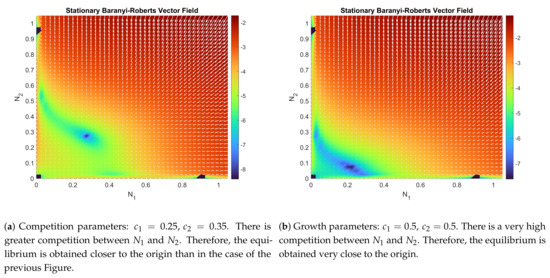
The Baranyi–Roberts system can be seen as a generalization of a family of multi-species Lotka–Volterra type interaction systems (see [34]). These systems can be classified as competition, mutualism, and predation systems (see [35,36]). Despite the classical and well-studied nature of these systems, finding the stability properties of (9) and (10) is tremendously complicated. We have been able to obtain an asymptotic stability result through linearization of system (9) and (10). However, numerical simulations show that the unique interior equilibrium point for the system (9) and (10) is a globally asymptotically stable point, and its attraction region is the entire initial set , except for the other three trivial equilibrium points (see Figure 1 and Figure 2). In particular,
has three trivial solutions, and . But there is another one in the interior of D, which can be found through a numerical root finder. Figure 1 and Figure 2 show the vector field and how the parameters affect the dynamics of the system.
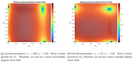
Figure 1.
Comparison of the flow function and its log-magnitude, , given by the Baranyi–Roberts system (9) and (10) with the set of parameters described in each figure, and in both figures. In darker color, the four equilibrium points that are given by the solutions of the nonlinear system (11) and (12).
Let us analyze the asymptotic behavior of the Baranyi–Roberts system (9) and (10). Let be its unique interior equilibrium point. Let the flow function be defined as
whose differential matrix at is
Notice that, to calculate the matrix , we have first computed and at , and we have then applied the equilibrium condition that is given by Equations (11) and (12).
Lyapunov’s indirect method [37] (Section 3.3) consists of studying the asymptotic behavior of a system by analyzing the asymptotic behavior of its linearized counterpart. It is widely used when studying highly nonlinear systems, where using Lyapunov functions may not provide enough information to discuss the stability of an equilibrium point (see [37] and references therein). The result may be stated in our case, as follows:
Theorem 2.
([37] (Th. 3.7)). Letbe an equilibrium point for the nonlinear system
whereand D is a neighborhood of the equilibrium point. Let
Subsequently, denoting ℜ as the real part of a complex number, the following statements are verified.
- The equilibrium point is stable iffor all eigenvaluesof A.
- The equilibrium point is unstable iffor one or more eigenvalues of A.
In our case, the eigenvalues for the matrix are obtained as the roots of the characteristic polynomial , where is the two-dimensional identity matrix. They can be determined by the following expression
where denotes the trace of the matrix and denotes the determinant of the matrix. It can be easily seen by using Equation (14), is negative for any set of admissible parameters. However, we can prove that the determinant is positive in certain cases. Indeed,
It is obvious that the sign of the determinant will only depend on the sign of . Therefore, if , then Theorem 2 assures that is a stable equilibrium point. It can be checked that all cases seen in Figure 1a and Figure 2b verify this last inequality (particular values of the parameters can be seen in the captions).
Now, let us consider the Baranyi–Roberts system (9) and (10) in the mean square sense with random initial conditions; that is, is a random vector that is defined in a common complete probability space. Local asymptotic stability sheds light upon the long-time behavior of the 1-PDF of the solution stochastic process . Theorem 1 states that the 1-PDF verifies the IVP (3) and (4) along with the Neumann boundary condition; that is
where is the vector flow function that is defined by (13).
Now, let be the local region of attraction of that is given by Theorem 2. Numerical computations show that the interior equilibrium point is actually globally stable so an attempt to compute the exact attraction region will not be made. The fact that Theorem 2 assures the existence of an attraction region will allow to obtain the 1-PDF asymptotic state. If the entire initial density is concentrated inside U, , then the asymptotic state of will be the Dirac delta function centered at ; that is, (see [38] (Lesson 27)). Let be a smooth function with compact support vanishing outside D; that is, . Subsequently,
because it has been assumed that the initial condition almost surely has realizations inside U. We have also used the fact that the exact solution along the characteristics is known, that all characteristic curves starting inside U will converge monotonically to , and that the total density inside the region of attraction is conserved (see Equation (6)). Later on, we will see that this is verified by the numerical simulations.
3. Assigning Reliable Probability Distributions to the Initial Conditions
The Principle of Maximum Entropy (PME) (see [29]) allows for assigning statistical distributions to some variables. It is based on maximizing the informational concept of differential entropy (see [39]), which is a measure defining the lack of knowledge of a random variable.
Given a random variable Y, with its associated PDF , the differential entropy or Shannon’s entropy (see [40]) is given by
where is the domain of the random variable Y (see [39] (Section 2.2)). This value quantifies the loss of information of a random variable; the less the information, the higher the entropy. In the extant literature, several contributions have applied PME to assign reliable statistical distributions for random variables (see [41,42,43]).
In order to assign reliable probabilistic distributions to a random variable, Y, the PME seeks for a PDF, , by maximizing the functional subject to the available information for the unknown random variable, such as the domain , its integral is the unit (), the mean , and other available higher moments , . Specifically, one solves the following optimization problem
where are the k-order moments, which are usually computed by metadata, samples, etc.
The general form of the density, , maximizing given , is given by
where the set is formed by the so-called Lagrange multipliers of the optimization problem (see [44] (Th. 1, Ch.8) and [29]).
In the setting of this contribution, the PME will be applied to assign a reliable PDF to the 2D sample data at time , i.e., the two-dimensional vector of initial conditions. Cell densities grow in separate cultures before being introduced in the same culture, according to the experimental procedure described in [28]. Therefore, it is logical to assume that the two initial random variables in system (9) and (10), which model the time evolution of the joint PDF in mixed culture, have statistically independent densities. Therefore, the joint PDF, as represented by in (3) and (4), can be expressed by for all . In our application, we will determine both and by separately using the PME in each cell culture population.
4. Application to Study Microbial Growth in a Competitive Environment
This section is devoted to apply the theoretical findings that are described above to study the growth of two microbial strains who compete for the same resources and space. It is important to remark that, to measure volumes and densities of microbial strains, it is necessary to use electronic devices that may have certain measurement errors. In order to account for this error, multiple measurements of the densities have been carried out (see [28] (Sec. Materials and Methods) for more details). Table 1 collects the mean and the standard deviation of all volumetric density measurements for the two microbial strains (denoted by Green Strain and Red Strain) at several time instants.

Table 1.
Mean and variance of the optical densities (OD) at different time instants of the two E. coli strains in mono-culture growth [28] (Experiment B).
Using the Baranyi–Roberts dynamical system described in (9) and (10), we study how the Green Strain and Red Strain compete in the same culture medium. Because the objective of this contribution is to illustrate the applicability of the proposed method in a real scenario, we will assume that the data collected in Table 1 show data from cells in a competitive mixed-culture, despite not being the case. Our data has intrinsic uncertainty given by measurement errors (epistemic uncertainty), so it seems reasonable to consider a randomized model, as it can be observed in Table 1. To do so, some of the model parameters are treated as random variables instead of deterministic values.
In this contribution, we perform a first step in the spirit of introducing uncertainties in the Baranyi–Roberts model by considering that the initial conditions, and , of the IVP (9) and (10) are independent random variables. They represent, respectively, the initial volumetric density of the Green Strain and Red Strain, which have been introduced in the culture medium. Then, taking into account the values of the means, and and of the standard deviations, and , (equivalently of the first and second moments) of and (see Table 1), we have applied the PME method to assign probability distributions, and , to and , respectively. This yields
where the values for the coefficients are given in Table 2. Therefore, the joint PDF, , of the initial condition of the Baranyi-Roberts system (9) and (10) is .
Table 2.
Lagrange multipliers for the Principle of Maximum Entropy (PME) problem. Optimization has been performed by using the fsolve built-in algorithm in MATLAB and following the steps described in Section 3. Data used to perform the optimization is located in Table A1 (see Appendix A).
Now that the joint PDF of the initial condition of IVP (9) and (10) has been determined, we can apply Theorem 1, which asserts that the solution of the PDE that is given in (3) and (4) defines the 1-PDF of the solution stochastic process of the Baranyi–Roberts system. Unfortunately, a closed form of the solution of the Liouville–Gibbs PDE is not affordable in our case and, consequently, we have used the DCU numerical scheme to approximate the solution of the Liouville–Gibbs PDE for every fixed time instant t. This numerical scheme is given by
where , , , and . The stability and convergence properties of this numerical scheme are analyzed in [26] (Chap. 20). Most finite volume schemes developed for two-dimensional (2D) hyperbolic PDEs are modified versions of the DCU, by adding correction terms, flux limiters and/or reconstruction algorithms in order to control the dissipation loss or possible instabilities from such a simple scheme and obtain very sharp and exact solutions in very few time-steps. The main advantage of the DCU scheme (18) and (20) is that it easy implementation and that it is very fast due to the fact that no extra terms are involved in the computation. The Courant–Friedrichs–Lewy (CFL) conditions are the space and time discretization size conditions, used in every PDE numerical solver, in order to assure stability and convergence of the numerical method to the true solution of the problem. In the particular case of the DCU scheme, the following CFL condition must be verified
where , and refer to the size of the space meshing in the x-direction, size of the meshing in the y-direction, and the time meshing, respectively. In the computations performed in this contribution, we have chosen , and . Once the numerical scheme to approximate the 1-PDF of the solution stochastic process of the Baranyi-Roberts model has been constructed, the model parameter values which best describe the data shown in Table 1 are searched through a specific optimization procedure. As indicated in the Introduction section, this has been done by applying the optimization technique known as PSO. In the next section, the entire computational procedure is described.
5. Computational Procedure Design
The PSO is a bio-inspired optimization algorithm that operates using rules that are similar to the behavior of swarms of birds that try to explore and exploit a certain region to find food (see [30]). The PSO algorithm generates a family of possible solutions (swarm of birds) in the given parametrical search space. It then updates, or evolves, the positions and velocities of the swarm over every iteration to minimize the Fitness Function (). Observe that the data in Table 1 correspond to the initial growth stage of both strains, therefore the specific growth rates and have a greater influence in the dynamics than the rest of the model parameters. Consequently, the PSO algorithm will be applied to determine the specific growth rates and , while the rest of model parameters (, , , , , and ) have been taken from [28] (see Table 3).
Table 3.
Parameters for the Baranyi–Roberts system after performing the optimization procedure. Note that we have only determined the growth parameters and , while the others have been taken from [28] (Experiment B).
For a given pair of growth parameters and , the (the error function to be minimized) is defined by the following steps:
- Step 1:
- Compute a discrete approximation of the 1-PDF at the time instants (in hours) by numerically solving the Liouville–Gibbs PDE, in the region , using the DCU scheme (18)–(20). We take the joint PDF given by the product of (16) and (17), with the parameters in Table 2, as the initial condition. We also consider null Neumann boundary conditions and the meshing parameters seen at the end of the previous section. This step gives a set of discrete values for each time instant . We use the notation of (18)–(20).
- Step 2:
- Compute the means at each time instant, and , using the values of and the composite 1/3 Simpson’s rule (see [45] (Chap. 25)) in each integration dimension; that is, we compute an approximation of (7) at each time instant.
- Step 3:
- Once the means for have been computed, which is and , we obtain the total error, denoted by , where each summand is the relative error between the aforementioned means and the sample data, and , as shown in Table 1,where
Once the fitness function has been defined, the PSO algorithm is applied to seek suitable growth parameters and .
6. Results
This section is aimed at showing the results obtained by implementing the procedure that is described in the previous section. Recall that the objective is to find the optimal values of and so that the mean of the 1-PDF given by the numerical scheme and the empirical mean of the data are as close as possible. To do so, the built-in MATLAB function particleswarm (see [46,47,48]) has been used to minimize the , defined through the three steps described in Section 5. Multiple different procedures have been executed at the same time in order to avoid the effect of randomness coming from generating the initial positions of the particles in PSO algorithm. The obtained results are close enough to guarantee that we can neglect the above-mentioned effect of randomness.
The procedure with the best results took over 7 h to reach a suitable minimum for the . The procedure has been carried out on an Ubuntu 16.04.7 LTS-based computer with a quad-core, 16-thread, Intel Xeon E5-4620 processor with 512 GB of RAM. Table 3 shows the values of the optimized parameters, and .
Figure 3 shows the punctual and accumulative errors defined, respectively, by and defined in expressions (22) and (21). We observe that the relative error decreases as time goes on. Figure 4 and Figure 5 show the vector field for the parameters in Table 3. In Figure 6a,b, we have performed a graphical comparison between the sampled data and the approximation obtained by our stochastic model for both Green and Red Strains. Both of the plots provide evidence of a very good fitting. Furthermore, the time evolution of the joint PDF of the solution stochastic process can be seen in Figure 7a–e. However, the maximum height of the joint PDF decreases very rapidly (observe the magnitude of the lateral colored bar), which means that the variance of the solution increases from diffusion, probably due to the DCU numerical scheme’s nature, as it can be seen in Figure 7a–e.
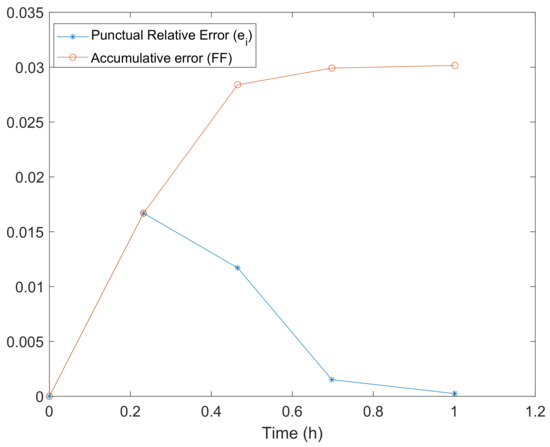
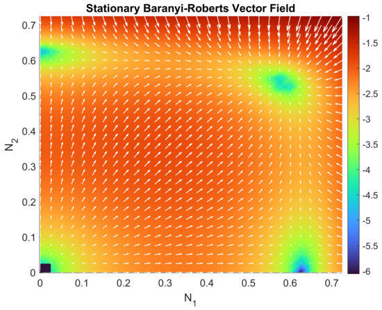
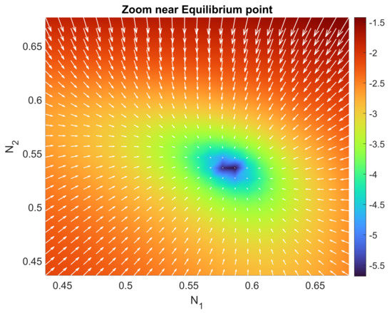
Figure 5.
Zoomed-up view of Figure 4 in a neighborhood of the interior equilibrium point . We can see how it clearly attracts all of the points surrounding the equilibrium point.
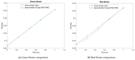
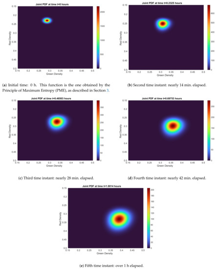
Figure 7.
Joint 1-PDF evolution of the solution stochastic process in every time instant given by data from Table 1. It can be seen how variance, which is reflected by the width/height ratio, grows. Take into account that the color bar is not fixed and, therefore, it re-scales itself at every time instant.
Predicting or extrapolating the dynamics of complex and highly parameterizable systems with randomness is a very difficult task. In our model setting, and after the previous validation process, we are interested in predicting the volumetric density of both strains of bacteria, since such future projections allow for the control of the biological culture. In Figure 8a,b, we show the predictions for Green and Red Strains over the time instants , , , and h. Comparing these figures with the ones that were collected in [28] (Experiment B), we observe that the stochastic model is able to capture the dynamics of volumetric density for the two strains of bacteria. This result has been obtained by only considering randomness in the initial conditions and adjusting the model parameters and .
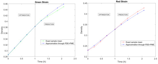
Figure 8.
Optimization, as computed in Section 5, and prediction of the mean paths of the solution stochastic process. The available data span over 2 h of measurements.
7. Conclusions
In this contribution, a procedure to quantify uncertainty in random dynamical systems has been defined and applied to a biological model. Specifically, we have made use of a result linking the first probability density function of the solution stochastic process of a random dynamical system with the classical Liouville–Gibbs Partial Differential Equation, whose solution, at every time instant, has been obtained using a finite volume numerical scheme. Using real data from experiments that were performed in the literature and the Principle of Maximum Entropy, a reliable probability density to the initial condition of the dynamical system has been assigned. We have successfully optimized two key model parameters, representing the growth rates of both types of strains of bacteria, so that the mean of the solution stochastic process is as close as possible to the real sample mean. The optimal values were obtained using the Particle Swarm Optimization algorithm. Because the original system depends on more model parameters that are susceptible to being randomized, in the forthcoming work we plan to address the full randomization of the model as well as implement higher order numerical solvers to better calibrate model parameters and perform more accurate predictions. We think that tackling this generalization of the uncertainty quantification procedure presented in our contribution will lead to challenging questions regarding the numerical solution of the corresponding Liouville–Gibbs equation.
Author Contributions
Software, V.J.B. and C.B.S.; formal analysis, V.J.B., C.B.S. and J.C.C.; investigation, V.J.B., C.B.S. and J.C.C.; writing—original draft preparation, V.J.B., C.B.S., J.C.C. and R.J.V.M.; writing—review and editing, V.J.B., C.B.S., J.C.C. and R.J.V.M.; supervision, J.C.C. and R.J.V.M.; funding acquisition, J.C.C. All authors have read and agreed to the published version of the manuscript.
Funding
This work has been supported by the Spanish Ministerio de Economía, Industria y Competitividad (MINECO), the Agencia Estatal de Investigación (AEI) and Fondo Europeo de Desarrollo Regional (FEDER UE) grant MTM2017-89664-P.
Data Availability Statement
Data can be found within the article and in [28].
Conflicts of Interest
The authors declare that they do not have any conflict of interest.
Appendix A. Dataset for Parameter Optimization
Table A1.
Density (OD) measurements of the Green Strain and Red Strain at initial time ( h). This data is used to estimate the parameters in Table 2. Note that more measurements were taken for the Green Strain than for the Red Strain. Complete data sources are available in [28].
Table A1.
Density (OD) measurements of the Green Strain and Red Strain at initial time ( h). This data is used to estimate the parameters in Table 2. Note that more measurements were taken for the Green Strain than for the Red Strain. Complete data sources are available in [28].
| Density (OD) of Green Strain | Density (OD) of Red Strain |
|---|---|
| 0.2803 | 0.2199 |
| 0.2902 | 0.2347 |
| 0.2778 | 0.2304 |
| 0.2768 | 0.2340 |
| 0.2860 | 0.2350 |
| 0.2996 | 0.2382 |
| 0.2833 | 0.2247 |
| 0.2968 | 0.2263 |
| 0.2972 | 0.2262 |
| 0.2778 | 0.2266 |
| 0.2945 | 0.2363 |
| 0.3017 | 0.2290 |
| 0.2791 | 0.2260 |
| 0.2873 | |
| 0.2989 | |
| 0.2772 | |
| 0.2776 | |
| 0.2832 | |
| 0.2796 | |
| 0.2852 | |
| 0.2953 | |
| 0.2707 | |
| 0.2868 | |
| 0.2898 |
References
- Iacus, S. Simulation and Inference for Stochastic Differential Equations: With R Examples; Springer: Berlin/Heidelberg, Germany, 2008; Volume 1. [Google Scholar] [CrossRef]
- Allen, E. Modeling with Itô Stochastic Differential Equations. In Mathematical Modelling: Theory and Applications; Springer Science & Business Media B.V.: Amsterdam, The Netherlands, 2007. [Google Scholar]
- Contreras-Reyes, J.E. Chaotic systems with asymmetric heavy-tailed noise: Application to 3D attractors. Chaos Solitons Fractals 2021, 145, 110820. [Google Scholar] [CrossRef]
- Caraballo, T.; Colucci, R.; López de la Cruz, J.; Rapaport, A. A way to model stochastic perturbations in population dynamics models with bounded realizations. Commun. Nonlinear Sci. Numer. Simul. 2019, 77, 239–257. [Google Scholar] [CrossRef]
- Loève, M. Probability Theory I; Volume 45, Graduate Texts in Mathematics; Springer: New York, NY, USA, 1977. [Google Scholar]
- Neckel, T.; Rupp, F. Random Differential Equations in Scientific Computing; Versita: London, UK, 2013. [Google Scholar]
- Soong, T.T. Random Differential Equations in Science and Engineering; Academic Press: New York, NY, USA, 1973. [Google Scholar]
- Wong, E.; Hajek, B. Stochastic Processes in Engineering System; Springer: New York, NY, USA, 1985. [Google Scholar]
- Coffey, W.; Kalmykov, Y.P.; Titov, S.; Mulligan, W. Semiclassical Klein-Kramers and Smoluchowski equations for the Brownian motion of a particle in an external potential. J. Phys. A Math. Theor. 2006, 40, F91. [Google Scholar] [CrossRef]
- Risken, H. The Fokker–Planck Equation Method of Solution and Applications; Springer: Berlin, Germany, 1989. [Google Scholar]
- Hesam, S.; Nazemi, A.R.; Haghbin, A. Analytical solution for the Fokker–Planck equation by differential transform method. Sci. Iran. 2012, 19, 1140–1145. [Google Scholar] [CrossRef]
- Lakestani, M.; Dehghan, M. Numerical solution of Fokker–Planck equation using the cubic B-spline scaling functions. Numer. Methods Partial Differ. Equ. 2009, 25, 418–429. [Google Scholar] [CrossRef]
- Mao, X.; Yua, C.; Yin, G. Numerical method for stationary distribution of stochastic differential equations with Markovian switching. J. Comput. Appl. Math. 2005, 174. [Google Scholar] [CrossRef]
- Calatayud, J.; Cortés, J.; Dorini, F.; Jornet, M. On a stochastic logistic population model with time-varying carrying capacity. Comput. Appl. Math. 2020, 39, 288. [Google Scholar] [CrossRef]
- Dorini, F.A.; Cecconello, M.S.; Dorini, M.B. On the logistic equation subject to uncertainties in the environmental carrying capacity and initial population density. Commun. Nonlinear Sci. Numer. Simul. 2016, 33, 160–173. [Google Scholar] [CrossRef]
- Kroese, D.; Taimre, T.; Botev, Z. Handbook of Monte Carlo Methods; John Wiley & Sons: Hoboken, NJ, USA, 2011. [Google Scholar] [CrossRef]
- Barbu, A.; Zhu, S. Monte Carlo Methods; Springer: Singapore, 2020. [Google Scholar] [CrossRef]
- Marelli, S.; Wicaksono, D.; Sudret, B. The UQLAB project: Steps toward a global uncertainty quantification community. In Proceedings of the 13th International Conference on Applications of Statistics and Probability in Civil Engineering (ICASP13), Seoul, Korea, 26–30 May 2019. [Google Scholar] [CrossRef]
- Schöbi, R.; Sudret, B.; Marelli, S. Rare Event Estimation Using Polynomial-Chaos Kriging. ASCE-ASME J. Risk Uncertain. Eng. Syst. Part A Civ. Eng. 2016, 500, D4016002. [Google Scholar] [CrossRef]
- Santambrogio, F. Optimal Transport for Applied Mathematicians. Calculus of Variations, PDEs and Modeling; Progress in Nonlinear Differential Equations and their Applications; Birkhäuser: Basel, Switzerland, 2015. [Google Scholar]
- Bevia, V.; Burgos, C.; Cortés, J.C.; Navarro-Quiles, A.; Villanueva, R.J. Analysing Differential Equations with Uncertainties via the Liouville-Gibbs Theorem: Theory and Applications. In Computational Mathematics and Applications; Zeidan, D., Padhi, S., Burqan, A., Ueberholz, P., Eds.; Springer: Singapore, 2020; pp. 1–23. [Google Scholar] [CrossRef]
- Evans, L. Partial Differential Equations; American Mathematical Society: Providence, RI, USA, 2010. [Google Scholar]
- Tadmor, E. A review of numerical methods for nonlinear partial differential equations. Bull. Am. Math. Soc. 2012, 49, 507–554. [Google Scholar] [CrossRef]
- Barth, T.; Herbin, R.; Ohlberger, M. Finite Volume Methods: Foundation and Analysis. In Encyclopedia of Computational Mechanics, 2nd ed.; John Wiley & Sons, Ltd.: Hoboken, NJ, USA, 2017. [Google Scholar] [CrossRef]
- Moukalled, F.; Mangani, L.; Darwish, M. The Finite Volume Method in Computational Fluid Dynamics: An Advanced Introduction with OpenFOAM and Matlab; Springer: Cham, Switzerland, 2015; Volume 113. [Google Scholar] [CrossRef]
- LeVeque, R.J. Finite Volume Methods for Hyperbolic Problems. In Cambridge Texts in Applied Mathematics; Cambridge University Press: Cambridge, UK, 2002. [Google Scholar] [CrossRef]
- Weisman, R.; Majji, M.; Alfriend, K. Solution of liouville’s equation for uncertainty characterization of the main problem in satellite theory. CMES Comput. Model. Eng. Sci. 2016, 111, 269–304. [Google Scholar]
- Ram, Y.; Dellus-Gur, E.; Bibi, M.; Karkare, K.; Obolski, U.; Feldman, M.W.; Cooper, T.F.; Berman, J.; Hadany, L. Predicting microbial growth in a mixed culture from growth curve data. Proc. Natl. Acad. Sci. USA 2019, 116, 14698–14707. [Google Scholar] [CrossRef]
- Jaynes, E.T. Information Theory and Statistical Mechanics. Phys. Rev. 1957, 106, 620–630. [Google Scholar] [CrossRef]
- Khemka, N.; Jacob, C. Exploratory Toolkit for Evolutionary and Swarm-Based Optimization. Math. J. 2008, 11, 376. [Google Scholar] [CrossRef]
- Burgos-Simón, C.; García-Medina, N.; Martínez-Rodríguez, D.; Villanueva, R.J. Mathematical modeling of the dynamics of the bladder cancer and the immune response applied to a patient: Evolution and short-term prediction. Math. Methods Appl. Sci. 2019, 42, 5746–5757. [Google Scholar] [CrossRef]
- Sundararaj, V. Optimised denoising scheme via opposition-based self-adaptive learning PSO algorithm for wavelet-based ECG signal noise reduction. Int. J. Biomed. Eng. Technol. 2017, 31, 325. [Google Scholar] [CrossRef]
- Mosayebi, R.; Bahrami, F. A modified particle swarm optimization algorithm for parameter estimation of a biological system. Theor. Biol. Med Model. 2018, 15, 17. [Google Scholar] [CrossRef] [PubMed]
- Goh, B.S. Global Stability in Many-Species Systems. Am. Nat. 1977, 111, 135–143. [Google Scholar] [CrossRef]
- Waltman, P.; Society for Industrial and Applied Mathematics; The Conference Board of the Mathematical Sciences; National Science Foundation. Competition Models in Population Biology; CBMS-NSF Regional Conference Series in Applied Mathematics; Society for Industrial and Applied Mathematics: Philadelphia, PA, USA, 1983. [Google Scholar]
- Goh, B.S. Stability in Models of Mutualism. Am. Nat. 1979, 113, 261–275. [Google Scholar] [CrossRef]
- Khalil, H.K. Nonlinear Systems, 3rd ed.; Prentice-Hall: Upper Saddle River, NJ, USA, 2002. [Google Scholar]
- Gasquet, C.; Witomski, P. Fourier Analysis and Applications. Filtering, Numerical Computation, Wavelets; Springer: Berlin/Heidelberg, Germany, 1998. [Google Scholar]
- Michalowicz, J.; Nichols, J.; Bucholtz, F. Handbook of Differential Entropy, 1st ed.; Chapman and Hall/CRC: New York, NY, USA, 2013. [Google Scholar]
- Shannon, C.E. A Mathematical Theory of Communication. Bell Syst. Tech. J. 1948, 27, 379–423. [Google Scholar] [CrossRef]
- Burgos Simón, C.; Cortés, J.; Martínez-Rodríguez, D.; Villanueva, R. Modeling breast tumor growth by a randomized logistic model: A computational approach to treat uncertainties via probability densities. Eur. Phys. J. Plus 2020, 135, 826. [Google Scholar] [CrossRef]
- Burgos, C.; Cortés, J.C.; Debbouche, A.; Villafuerte, L.; Villanueva, R.J. Random fractional generalized Airy differential equations: A probabilistic analysis using mean square calculus. Appl. Math. Comput. 2019, 352, 15–29. [Google Scholar] [CrossRef]
- Burgos, C.; Cortés, J.C.; Villafuerte, L.; Villanueva, R.J. Mean square convergent numerical solutions of random fractional differential equations: Approximations of moments and density. J. Comput. Appl. Math. 2020, 378, 112925. [Google Scholar] [CrossRef]
- Luenberger, D.G. Optimization by Vector Space Methods, 1st ed.; John Wiley & Sons, Inc.: New York, NY, USA, 1997. [Google Scholar]
- Riley, K.; Hobson, M.; Bence, S. Mathematical Methods for Physics and Engineering, 3rd ed.; Cambridge University Press: Cambridge, UK, 1999; Volume 67. [Google Scholar] [CrossRef]
- Kennedy, J.; Eberhart, R. Particle swarm optimization. In Proceedings of the ICNN’95—International Conference on Neural Networks, Perth, Australia, 27 November–1 December1 995; Volume 4, pp. 1942–1948. [CrossRef]
- Mezura-Montes, E.; Coello Coello, C.A. Constraint-handling in nature-inspired numerical optimization: Past, present and future. Swarm Evol. Comput. 2011, 1, 173–194. [Google Scholar] [CrossRef]
- Pedersen, M.E.H. Good Parameters for Particle Swarm Optimization; Hvass Laboratories: Copenhagen, Denmark, 2010. [Google Scholar]
Publisher’s Note: MDPI stays neutral with regard to jurisdictional claims in published maps and institutional affiliations. |
© 2021 by the authors. Licensee MDPI, Basel, Switzerland. This article is an open access article distributed under the terms and conditions of the Creative Commons Attribution (CC BY) license (http://creativecommons.org/licenses/by/4.0/).