Numerical Simulation for the Treatment of Nonlinear Predator–Prey Equations by Using the Finite Element Optimization Method

Abstract

This article aims to introduce an efficient simulation to obtain the solution for a dynamical–biological system, which is called the Lotka–Volterra system, involving predator–prey equations. The finite element method (FEM) is employed to solve this problem. This technique is based mainly upon the appropriate conversion of the proposed model to a system of algebraic equations. The resulting system is then constructed as a constrained optimization problem and optimized in order to get the unknown coefficients and, consequently, the solution itself. We call this combination of the two well-known methods the finite element optimization method (FEOM). We compare the obtained results with the solutions obtained by using the fourth-order Runge–Kutta method (RK4 method). The residual error function is evaluated, which supports the efficiency and the accuracy of the presented procedure. From the given results, we can say that the presented procedure provides an easy and efficient tool to investigate the solution for such models as those investigated in this paper.

1. Introduction

Nonlinear differential equations have kept attracting the interest of many researchers. Some authors have realized the need for finding new mathematical models of many real-life problems in such different areas as, for example, fluid mechanics, viscoelasticity, biology, physics, and engineering. Most nonlinear differential equations do not have an exact solution. Therefore, approximate and numerical techniques must be used (see [1,2,3,4]). For relevant further details about differential equations, together with their important properties and the tools and techniques used for them, one can see the works [5] (see also [6] for various developments involving ordinary differential equations as well as analogous fractional-order differential equations).

After the above-mentioned works, many researchers have successfully applied various numerical methods in this field (see, for example, [7]). Among these numerical methods, the finite element method (FEM) (see [8]) has some distinct advantages for handling this class of problems in which the coefficients for the solution can easily be found to exist after using any one of the available numerical programs. Here, we state the main advantages to this technique through the following points:

1.

FEM allows for easier modeling of complex geometrical and irregular shapes.

2.

FEM can be adapted to obtain the solution of the problem with a high degree of accuracy to decrease the need for physical prototypes in the design process.

3.

FEM is remarkably useful for certain time-dependent simulations, such as crash simulations in which deformations in one area depend upon deformations in another area.

In this paper, we apply the finite element optimization method (FEOM) to obtain the solution for the given problem. The outline of the paper is as follows:

• Section 2 is devoted to the presentation of the formulation of the Lotka–Volterra system;
• Section 3 is devoted to the construction and prediction of the solution by FEOM;
• Section 4 is devoted to the results and discussion;
• Section 5 presents the conclusions of this investigation.

2. The Model of the Lotka–Volterra System (with Two Predators and One Prey)

Predator–prey equations are a pair of nonlinear differential equations of the first order that are frequently used to describe the dynamics of biological systems in which two species interact with each other; one is a predator and the other is its prey. The studied model was presented by Samardzija [9], who proposed a two-predator and one-prey concept of the Lotka–Volterra system.

In our study, the proposed model for the predator–prey equations is defined as follows:

$$x^{\prime }\left(t\right)={\lambda }_{1}x\left(t\right)-{\lambda }_{2}x\left(t\right)y\left(t\right)+{\lambda }_3{\left[x\left(t\right)\right]}^2-{\lambda }_{4}z\left(t\right){\left[x\left(t\right)\right]}^2,$$

(1)

$$y^{\prime }\left(t\right)=-{\lambda }_{5}y\left(t\right)+{\lambda }_{6}x\left(t\right)y\left(t\right)$$

(2)

and

$$z^{\prime }\left(t\right)=-{\lambda }_{7}z\left(t\right)+{\lambda }_{4}z\left(t\right){\left[x\left(t\right)\right]}^2,$$

(3)

together with the following initial conditions:

$$x\left(0\right)=x_0,y\left(0\right)=y_0\mathrm{and}z\left(0\right)=z_0,$$

(4)

where a prime denotes differentiation with respect to t, $y\left(t\right)$ and $z\left(t\right)$ are the numbers of the predators at time t, $x\left(t\right)$ is the number of their prey at time t, and ${\lambda }_j(j=1,\dots ,7)$ are the parameters that represent the interaction between the three species involved (see also [10,11]). In our present work, we solve this problem in the interval $(0,t_f)=(0,8)$. For more details about this model, see the earlier work [9].

3. Procedure of Solution by the Finite Element Method (FEM)

The FEM is a powerful technique for solving differential equations and integral equations, as well as their fractional-order analogs. The basic concept is that the whole domain is divided into smaller elements of finite dimensions, called Finite Elements. It is one of the most versatile numerical techniques in modern engineering analysis and is employed to study diverse problems in such areas as, for example, fluid mechanics [12], heat transfer [13], chemical processing [14], solid mechanics [15], electrical systems, and many other fields.

The analysis of the finite element method is implemented through the following steps (see, for details, [16]):

1.

Finite-element discretization:

The whole domain is divided into a finite number of sub-domains, which is called the discretization of the domain. Each sub-domain is called an element. The collection of elements is called the finite-element mesh.

2.

Generation of the element equations:

• From the mesh, a typical element is isolated and the variational formulation of the given problem over the typical element is then constructed.
• An approximate solution of the variational problem is assumed and the element equations are formulated by substituting this solution into the above system.
• The element matrix, which is called the stiffness matrix, is constructed by using the element interpolation functions.

3.

Assembly of the element equations:

The algebraic equations so obtained are assembled by imposing the inter-element continuity conditions. This yields a large number of algebraic equations known as the global finite element model, which governs the whole domain.

4.

Imposition of the boundary conditions:

The essential and natural boundary conditions are imposed on the assembled equations.

5.

Solution a system of algebraic equations:

The obtained system of algebraic equations can be solved by any one of the appropriate numerical techniques.

3.1. Variational Formulation of the System

The variational form associated with Equations (1)–(3) over a typical linear element $(t_e,t_{e+1})$ is given by the following:

$${\int }_{t_e}^{t_{e+1}}{\varphi }_1\left[x^{\prime }\left(t\right)-{\lambda }_{1}x\left(t\right)+{\lambda }_{2}x\left(t\right)y\left(t\right)-{\lambda }_3{\left[x\left(t\right)\right]}^2+{\lambda }_{4}z\left(t\right){\left[x\left(t\right)\right]}^2\right]dt=0,$$

(5)

$${\int }_{t_e}^{t_{e+1}}{\varphi }_2\left[y^{\prime }\left(t\right)+{\lambda }_{5}y\left(t\right)-{\lambda }_{6}x\left(t\right)y\left(t\right)\right]dt=0$$

(6)

and

$${\int }_{t_e}^{t_{e+1}}{\varphi }_3\left[z^{\prime }\left(t\right)+{\lambda }_{7}z\left(t\right)-{\lambda }_{4}z\left(t\right){\left[x\left(t\right)\right]}^2\right]dt=0,$$

(7)

where ${\varphi }_1,$${\varphi }_2$ and ${\varphi }_3$ are arbitrary test functions and may be viewed as the variation in $x\left(t\right),$$y\left(t\right)$ and $z\left(t\right)$, respectively.

3.2. Finite Element Formulation of the Model

The finite element model may be obtained from the above equations by substituting finite element approximations of the following form:

$$x\left(t\right)=\sum _{\ell =1}^2{x}_{\ell }{\mathsf{{\rm Y}}}_{\ell },h\left(t\right)=\sum _{\ell =1}^2{y}_{\ell }{\mathsf{{\rm Y}}}_{\ell }\mathrm{and}z\left(t\right)=\sum _{\ell =1}^2{z}_{\ell }{\mathsf{{\rm Y}}}_{\ell },$$

(8)

together with

$${\varphi }_1={\varphi }_2={\varphi }_3={\mathsf{{\rm Y}}}_{\ell }(\ell =1,2).$$

In our computations, the shape functions of a typical element $(t_e,t_{e+1})$ are taken to be as follows:

Linear element:

$${\mathsf{{\rm Y}}}_1^e=\frac{t_{e+1}-t}{t_{e+1}-t_e},{\mathsf{{\rm Y}}}_2^e=\frac{t-t_e}{t_{e+1}-t_e}\mathrm{and}{t}_e\leqq t\leqq t_{e+1}.$$

(9)

Quadratic element:

$$\begin{array}{cc}\hfill & {\mathsf{{\rm Y}}}_1^e=\frac{(t_{e+1}-t_e-2t)(t_{e+1}-t)}{{(t_{e+1}-t_e)}^2},\hfill \\ \hfill & {\mathsf{{\rm Y}}}_2^e=\frac{4(t-t_e)(t_{e+1}-t)}{{(t_{e+1}-t_e)}^2},\hfill \\ \hfill & {\mathsf{{\rm Y}}}_3^e=-\frac{(t_{e+1}-t_e-2t)(t-t_e)}{{(t_{e+1}-t_e)}^2}\mathrm{and}{t}_e\leqq t\leqq t_{e+1}.\hfill \end{array}$$

(10)

The finite element model of the equations thus formed is given by the following:

$$\left(\begin{array}{ccc}\left[K^{12}\right]& \left[K^{12}\right]& \left[K^{13}\right]\\ \left[K^{21}\right]& \left[K^{22}\right]& \left[K^{23}\right]\\ \left[K^{31}\right]& \left[K^{32}\right]& \left[K^{33}\right]\end{array}\right)\left(\begin{array}{c}\left\{x\right\}\\ \left\{y\right\}\\ \left\{z\right\}\end{array}\right)=\left(\begin{array}{c}\left\{b^1\right\}\\ \left\{b^2\right\}\\ \left\{b^3\right\}\end{array}\right),$$

(11)

where $\left[K^{rs}\right]$ and $\left[b^r\right]$ ($r,s=1,2,3$) are defined as follows:

$$\begin{array}{cc}\hfill & \left[K_{ij}^{11}\right]={\int }_{t_e}^{t_{e+1}}\left({\mathsf{{\rm Y}}}_i\frac{d{\mathsf{{\rm Y}}}_j}{dt}-{\lambda }_1{\mathsf{{\rm Y}}}_i{\mathsf{{\rm Y}}}_j\right)dt-{\lambda }_3{\int }_{t_e}^{t_{e+1}}\left({\mathsf{{\rm Y}}}_i\overline{x}{\mathsf{{\rm Y}}}_j\right)dt,\hfill \\ \hfill & \left[K_{ij}^{12}\right]={\lambda }_2{\int }_{t_e}^{t_{e+1}}\left({\mathsf{{\rm Y}}}_i\overline{x}{\mathsf{{\rm Y}}}_j\right)dt,\left[K_{ij}^{13}\right]={\lambda }_4{\int }_{t_e}^{t_{e+1}}\left({\mathsf{{\rm Y}}}_i\overline{x}{\mathsf{{\rm Y}}}_j\right)dt,\hfill \\ \hfill & \left[K_{ij}^{21}\right]=-{\lambda }_6{\int }_{t_e}^{t_{e+1}}\left({\mathsf{{\rm Y}}}_i\overline{y}{\mathsf{{\rm Y}}}_j\right)dt,\left[K_{ij}^{22}\right]={\int }_{t_e}^{t_{e+1}}\left({\mathsf{{\rm Y}}}_i\frac{d{\mathsf{{\rm Y}}}_j}{dt}+{\lambda }_5{\mathsf{{\rm Y}}}_i{\mathsf{{\rm Y}}}_j\right)dt,\hfill \\ \hfill & \left[K_{ij}^{23}\right]=0,\left[K_{ij}^{31}\right]=-{\lambda }_4{\int }_{t_e}^{t_{e+1}}\left({\mathsf{{\rm Y}}}_i\overline{z}{\mathsf{{\rm Y}}}_j\right)dt,\hfill \\ \hfill & \left[K_{ij}^{32}\right]=0,\left[K_{ij}^{33}\right]={\int }_{t_e}^{t_{e+1}}\left({\mathsf{{\rm Y}}}_i\frac{d{\mathsf{{\rm Y}}}_j}{dt}+{\lambda }_7{\mathsf{{\rm Y}}}_i{\mathsf{{\rm Y}}}_j\right)dt,\hfill \\ \hfill & b_i^1=0,b_i^2=0,\mathrm{and}{b}_i^3=0,\hfill \end{array}$$

(12)

in which

$$\overline{x}=\sum _{\ell =1}^2\overline{x_{\ell }}{\mathsf{{\rm Y}}}_{\ell },\overline{y}=\sum _{\ell =1}^2\overline{y_{\ell }}{\mathsf{{\rm Y}}}_{\ell },\mathrm{and}\overline{z}=\sum _{\ell =1}^2\overline{z_{\ell }}{\mathsf{{\rm Y}}}_{\ell }.$$

Each element matrix is of the order $6\times 6$. The entire flow domain is divided into a set of 800 line elements and, following the assembly of all of the element equations, a matrix of order $2403\times 2403$ is generated. The resulting system of equations is strongly nonlinear and recourse must be made to a robust iterative scheme to solve it. The system is linearized by incorporating the functions $\overline{x},\overline{y}$ and $\overline{z}$, which are assumed to be known. After applying the given boundary conditions, only a system of 2398 equations remains for finding the solution, which is performed by using a robust Gauss elimination method while maintaining an accuracy of 0.0001. A convergence criterion based on the relative difference between the current and previous iterations is employed. When these differences reach the desired accuracy, the solution is assumed to have converged and the iterative process is then terminated. The Gaussian quadrature is implemented for solving the integrations. However, the suitability of the shape functions varies from problem to problem. Due to the simple and efficient use in computations, linear, as well as quadratic, shape functions are used in the present problem. However, it is observed that the results do not vary considerably, indicating that both elements provide approximately the same accuracy.

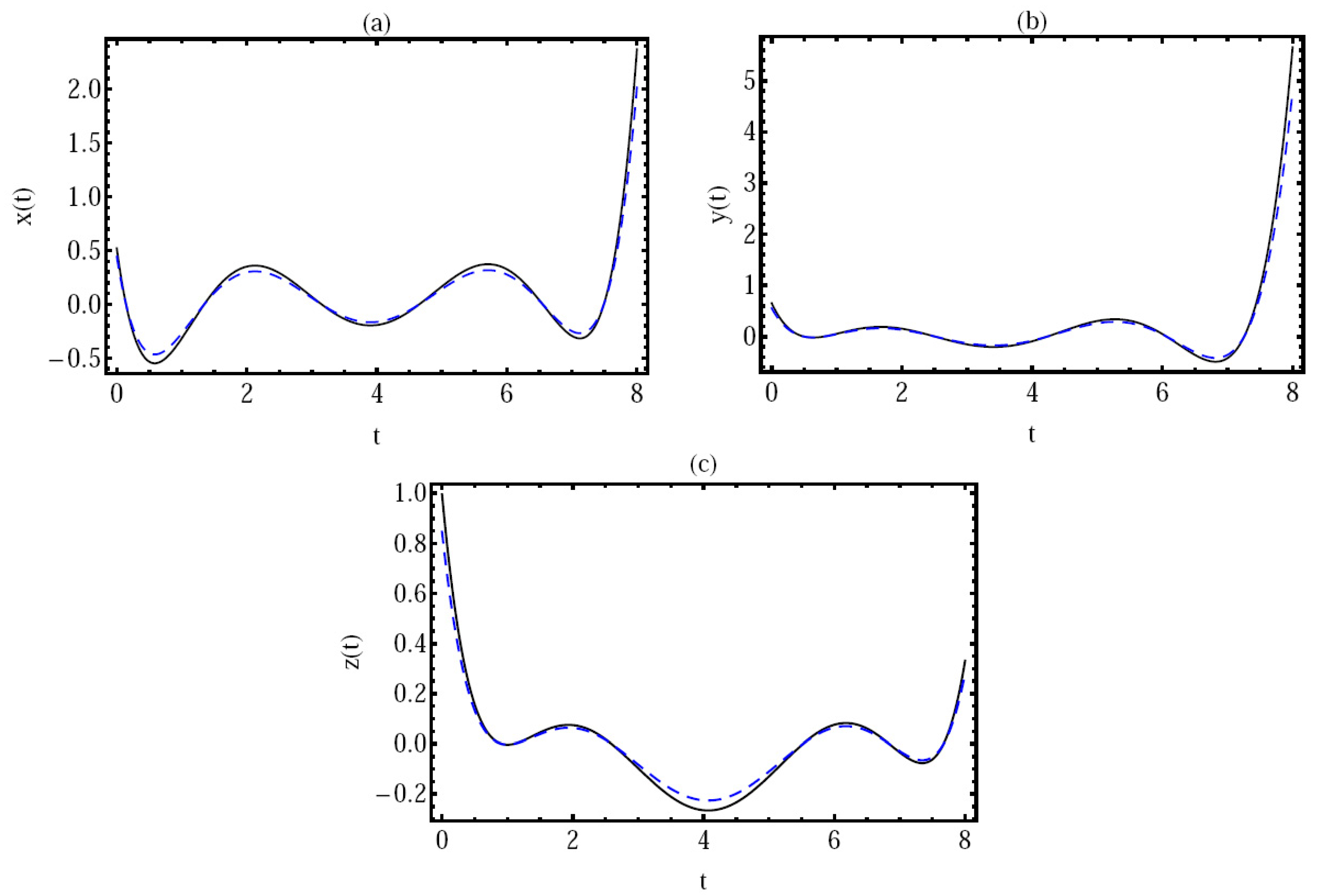
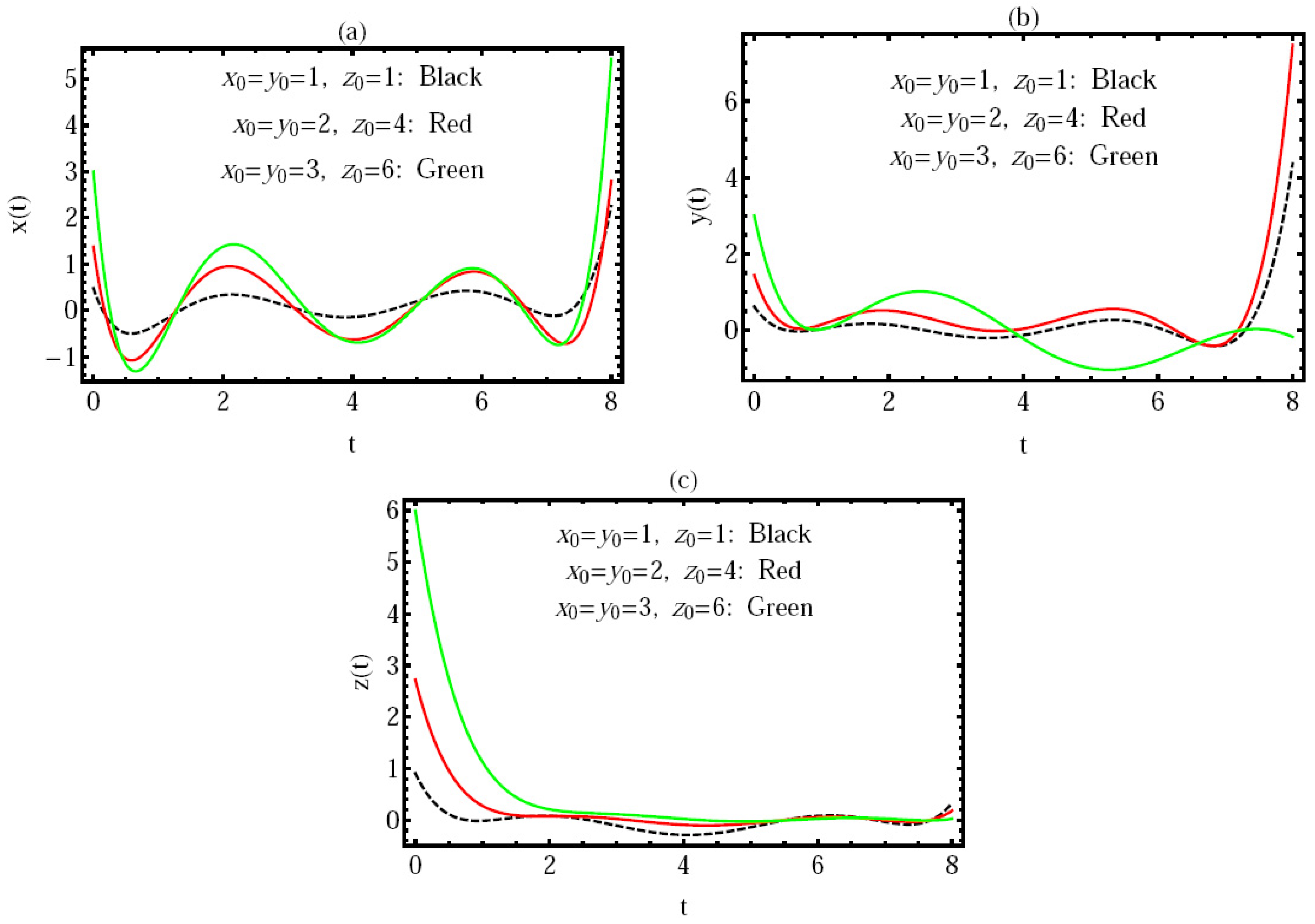
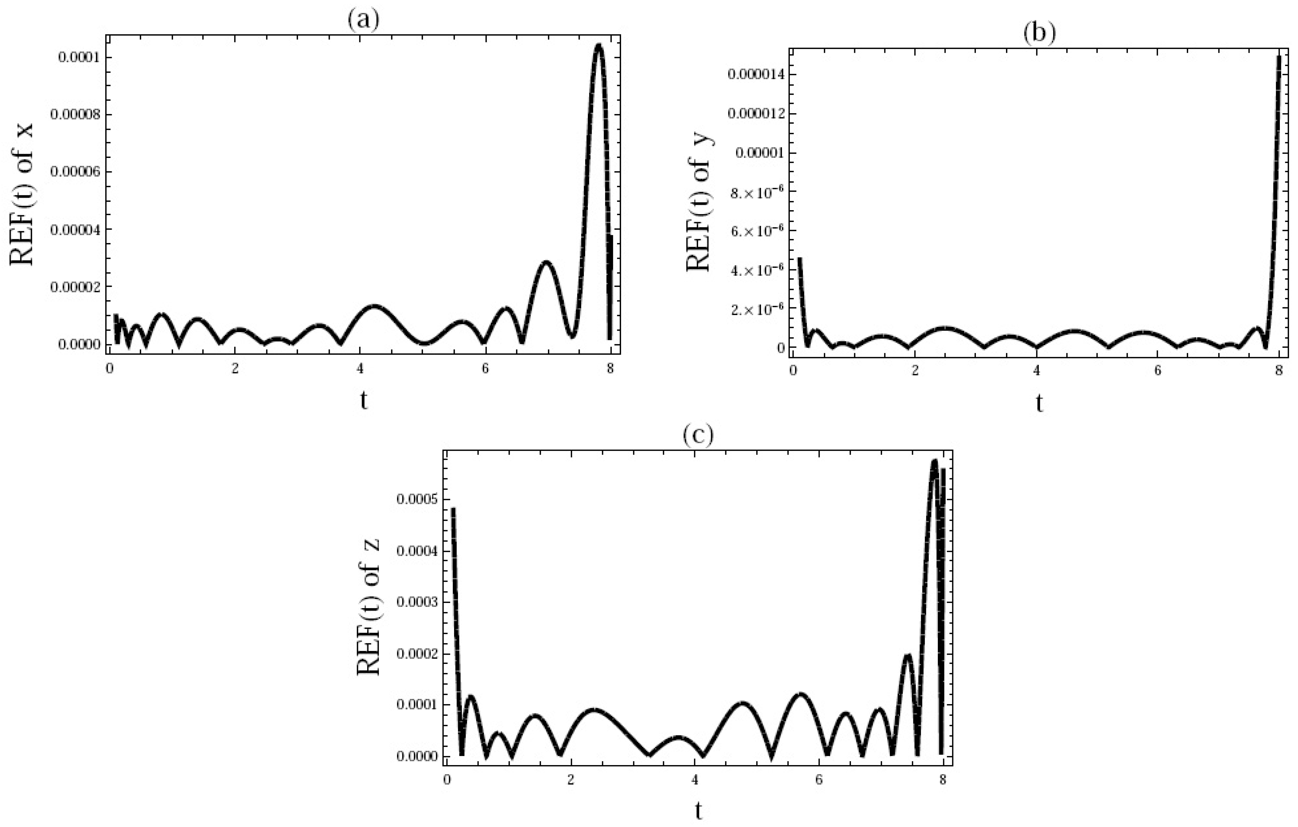
4. Numerical Simulation

Here, in this section, we present a numerical test example to verify the accuracy and the quality of the presented scheme. With this aim in view, we consider the systems (1) to (4) with different values of the parameters ${\lambda }_j(j=1,\dots ,7)$, as well as the initial conditions for $x_0,$$y_0$ and $z_0.$ Figure 1, Figure 2, Figure 3 and Figure 4 present the numerical simulation for the studied model by employing the technique that we have used in this paper.

In Figure 1, we present the behavior of the approximate solution by the proposed method (dotted line) and the fourth-order Runge–Kutta method (continuous line) in the interval ($0,8$) with the initial conditions $x_0=0.5,$$y_0=1$ and $z_0=1$ and with the parameters given by the following:

$${\lambda }_1={\lambda }_2={\lambda }_3={\lambda }_4=1,{\lambda }_5=2,{\lambda }_6=3\mathrm{and}{\lambda }_7=2.7.$$

In Figure 2, we present the behavior of the approximate solution via distinct values of the initial conditions in the interval ($0,8$) and with the parameters given by the following:

$${\lambda }_1={\lambda }_2={\lambda }_3={\lambda }_4=1,{\lambda }_5=2,{\lambda }_6=3\mathrm{and}{\lambda }_7=2.7.$$

In this situation, we take the following three cases:

i. 

$x_0=y_0=1,z_0=2$; (a) for the solution $x\left(t\right)$;

ii. 

$x_0=y_0=2,z_0=4$; (b) for the solution $y\left(t\right)$;

iii. 

$x_0=y_0=3,z_0=6$; (c) for the solution $z\left(t\right)$.

In Figure 3, we present the behavior of the approximate solution via distinct values of the parameters ${\lambda }_i(i=1,\dots ,7)$ together with $x_0=y_0=1$ and $z_0=2$ in the interval ($0,8$). In this situation, we take the following three cases:

i. 

${\lambda }_1={\lambda }_2={\lambda }_3={\lambda }_4=2,{\lambda }_5={\lambda }_6=1,{\lambda }_7=3$ (a);

ii. 

${\lambda }_1={\lambda }_2={\lambda }_3={\lambda }_4=3,{\lambda }_5={\lambda }_6=2,{\lambda }_7=4$ (b);

iii. 

${\lambda }_1={\lambda }_2={\lambda }_3={\lambda }_4=4,{\lambda }_5={\lambda }_6=3,{\lambda }_7=5$ (c).

In addition, in Figure 4, the residual error function (REF) is introduced at the initial conditions $x_0=y_0=1,$ and $z_0=2$, with the parameters given by the following:

$${\lambda }_1={\lambda }_2={\lambda }_3={\lambda }_4=1,{\lambda }_5=2,{\lambda }_6=3\mathrm{and}{\lambda }_7=2.7.$$

From these results, we can note that the behavior of the numerical solution depends on the values in the initial conditions and the included parameters ${\lambda }_j(j=1,\dots ,7)$. This confirms that the used method has been implemented in a good way for solving the proposed problem.

In order to validate our numerical solutions, we present a comparison of the REF in

Table 1. Comparison of the REF between FEOM and RK4 method.

	Relative Error—Present FEOM:			Relative Error—RK4:
$\mathit{t}$	$\mathit{x}\left(\mathit{t}\right)$	$\mathit{y}\left(\mathit{t}\right)$	$\mathit{z}\left(\mathit{t}\right)$	$\mathit{x}\left(\mathit{t}\right)$	$\mathit{y}\left(\mathit{t}\right)$	$\mathit{z}\left(\mathit{t}\right)$
0	3.15972 $\times {10}^{-9}$	4.85231 $\times {10}^{-8}$	5.98745 $\times {10}^{-8}$	3.12345 $\times {10}^{-7}$	1.65482 $\times {10}^{-7}$	2.35479 $\times {10}^{-7}$
1	3.75361 $\times {10}^{-8}$	4.98765 $\times {10}^{-7}$	1.85317 $\times {10}^{-7}$	0.96325 $\times {10}^{-7}$	2.74123 $\times {10}^{-7}$	1.85213 $\times {10}^{-7}$
2	2.85264 $\times {10}^{-8}$	0.05217 $\times {10}^{-8}$	1.85214 $\times {10}^{-8}$	6.36547 $\times {10}^{-6}$	2.96542 $\times {10}^{-7}$	9.85471 $\times {10}^{-7}$
3	2.12358 $\times {10}^{-8}$	4.98541 $\times {10}^{-8}$	3.65412 $\times {10}^{-9}$	9.75612 $\times {10}^{-7}$	2.95423 $\times {10}^{-6}$	1.95423 $\times {10}^{-6}$
4	4.32546 $\times {10}^{-8}$	6.02546 $\times {10}^{-9}$	5.85642 $\times {10}^{-8}$	9.95423 $\times {10}^{-7}$	5.35491 $\times {10}^{-7}$	1.32564 $\times {10}^{-7}$
5	7.85214 $\times {10}^{-8}$	0.32541 $\times {10}^{-7}$	6.65482 $\times {10}^{-8}$	3.02587 $\times {10}^{-7}$	3.65821 $\times {10}^{-7}$	9.78523 $\times {10}^{-7}$
6	1.12597 $\times {10}^{-8}$	2.32587 $\times {10}^{-8}$	5.95421 $\times {10}^{-7}$	0.65478 $\times {10}^{-6}$	1.32587 $\times {10}^{-6}$	4.58241 $\times {10}^{-7}$
7	8.65874 $\times {10}^{-9}$	2.32541 $\times {10}^{-8}$	6.96325 $\times {10}^{-8}$	4.74185 $\times {10}^{-7}$	3.00254 $\times {10}^{-6}$	1.21504 $\times {10}^{-6}$
8	1.25846 $\times {10}^{-8}$	3.24680 $\times {10}^{-8}$	5.25813 $\times {10}^{-9}$	7.89240 $\times {10}^{-7}$	9.11005 $\times {10}^{-7}$	1.90412 $\times {10}^{-7}$

at the initial conditions $x_0=y_0=2,$ and $z_0=3$, and with the parameters given by the following:

$${\lambda }_1={\lambda }_2={\lambda }_3={\lambda }_4=2,{\lambda }_5=0.8,{\lambda }_6=3\mathrm{and}{\lambda }_7=1.7.$$

This comparison shows the thoroughness of the proposed method in this article.

5. Conclusions

The proposed model is solved numerically by employing the finite element optimization method (FEOM). The resulting numerical solutions for the studied problem confirm that the presented technique is quite suitable to study this problem effectively. We can confirm also that, if we add extra terms from the series of the approximate solution, the errors will decrease. Finally, the numerical solutions with different values of the order n of approximation and the residual error function are computed to illustrate the validity of the proposed technique. The derived results also show that the given procedure provides an efficient tool to investigate the numerical solution for such models. On the other hand, in capturing this numerical analysis, our work may provide stronger physical meanings for performing future theoretical and computational analysis on this subject. All numerical results in this paper were obtained by using the Mathematica software.

References

1. Ali, M.R.; Hadhoud, A.R.; Srivastava, H. Solution of fractional Volterra-Fredholm integro-differential equations under mixed boundary conditions by using the HOBW method. Adv. Differ. Equ. 2019, 2019, 115. [Google Scholar] [CrossRef] [Green Version]
2. Homeier, H.H.; Srivastava, H.M.; Masjed-Jamei, M.; Moalemi, Z. Some weighted quadrature methods based upon the mean value theorems. Math. Methods Appl. Sci. 2021, 44, 3840–3856. [Google Scholar] [CrossRef]
3. Khader, M.M.; Sharma, R.P. Evaluating the unsteady MHD micropolar fluid flow past stretching/shirking sheet with heat source and thermal radiation: Implementing fourth order predictor-corrector FDM. Math. Comput. Simulat. 2021, 181, 333–350. [Google Scholar] [CrossRef]
4. Srivastava, H.M.; Iqbal, J.; Arif, M.; Khan, A.; Gasimov, Y.S.; Chinram, R. A new application of Gauss quadrature method for solving systems of nonlinear equations. Symmetry 2021, 13, 432. [Google Scholar] [CrossRef]
5. Srivastava, H.M.; Saad, K.M.; Khader, M.M. An efficient spectral collocation method for the dynamic simulation of the fractional epidemiological model of the Ebola virus. Chaos Solitons Fractals 2020, 140, 110174. [Google Scholar] [CrossRef] [PubMed]
6. Kilbas, A.A.; Srivastava, H.M.; Trujillo, J.J. Theory and Applications of Fractional Differential Equations. North-Holland Mathematical Studies; Elsevier (North-Holland) Science Publishers: Amsterdam, The Netherlands; London, UK; New York, NY, USA, 2006; Volume 204. [Google Scholar]
7. Garvie, M.R.; Burkardt, J.; Morgan, J. Simple finite element methods for approximating predator-prey dynamics in two dimensions using Matlab. Bull. Math. Biol. 2015, 77, 548–578. [Google Scholar] [CrossRef] [PubMed]
8. Khader, M.M.; Abualnaja, K.M. Galerkin-FEM for obtaining the numerical solution of the linear fractional Klein-Gordon equation. J. Appl. Anal. Comput. 2019, 9, 261–270. [Google Scholar] [CrossRef]
9. Bougoffa, L.; Khanfer, A. On the solutions of the generalized Lotka-Volterra system. In Proceedings of the ITM Web of Conferences, Moscow, Russia, 28–29 November 2019; pp. 1–6. [Google Scholar]
10. Atangana, A.; Gómez-Aguilar, J.F. A new derivative with normal distribution kernel: Theory, methods and applications. Phys. A Statist. Mech. Appl. 2017, 476, 1–14. [Google Scholar] [CrossRef]
11. Ghanbari, B.; Günerhan, H.; Srivastava, H.M. An application of the Atangana-Baleanu fractional derivative in mathematical biology: A three-species predator-prey model. Chaos Solitons Fractals 2020, 138, 109919. [Google Scholar] [CrossRef]
12. Bhargava, R.; Sharma, S.; Takhar, H.S.; Beg, O.A.; Bhargava, P. Numerical solutions for micropolar transport phenomena over a nonlinear stretching sheet. Nonlinear Anal. Model. Cont. 2007, 12, 45–63. [Google Scholar] [CrossRef]
13. Bathe, K.J. Finite Element Procedures; Prentice Hall, Pearson Education Incorporated: New York, NY, USA, 2006. [Google Scholar]
14. Lin, Y.-Y.; Lo, S.-P. Finite element modeling for chemical mechanical polishing process under different back pressures. J. Mater. Process. Technol. 2003, 140, 646–652. [Google Scholar] [CrossRef]
15. Hansbo, A.; Hansbo, P. A finite element method for the simulation of strong and weak discontinuities in solid mechanics. Comput. Methods Appl. Mech. Eng. 2004, 139, 3523–3540. [Google Scholar] [CrossRef]
16. Rana, P.; Bhargava, R. Flow and heat transfer of a nanofluid over a nonlinearly stretching sheet: A numerical study. Commun. Nonlinear Sci. Numer. Simulat. 2012, 17, 212–226. [Google Scholar] [CrossRef]
Figure 1. Behavior of the approximate solution by the proposed method (dots line) and the RK4 (continuous line).
Fractalfract 05 00056 g001
Figure 2. Behavior of the approximate solution via different values of x 0 , y 0 and z 0 .
Fractalfract 05 00056 g002
Figure 3. Behavior of the approximate solution via different values of the parameters λ j ( j = 1 , , 7 ) .
Fractalfract 05 00056 g003aFractalfract 05 00056 g003b
Figure 4. The REF of the solutions.
Fractalfract 05 00056 g004