A Grey System Approach for Estimating the Hölderian Regularity with an Application to Algerian Well Log Data

Abstract

The Hölderian regularity is an important mathematical feature of a signal, connected with the physical nature of the measured parameter. Many algorithms have been proposed in literature for estimating the local Hölder exponent value, but all of them lead to biased estimates. This paper attempts to apply the grey system theory (GST) on the raw signal for improving the accuracy of Hölderian regularity estimation. First, synthetic logs data are generated by the successive random additions (SRA) method with different types of Hölder functions. The application on these simulated signals shows that the Hölder functions estimated by the GST are more precise than those derived from the raw data. Additionally, noisy signals are considered for the same experiment, and more accurate regularity is obtained using signals processed using GST. Second, the proposed technique is implemented on well log data measured at an Algerian exploration borehole. It is demonstrated that the regularity determined from the well logs analyzed by the GST is more reliable than that inferred from the raw data. In addition, the obtained Hölder functions almost reflect the lithological discontinuities encountered by the well. To conclude, the GST is a powerful tool for enhancing the estimation of the Hölderian regularity of signals.

1. Introduction

The Hölderian regularity is a robust property of physical signals. The understanding of its time/space variations allows to extract meaningful information related to the physical nature of the analyzed signal.

To describe physical signals exhibiting spatial (or time)-dependent regularity, many stochastic fractal models have been suggested. The most generalized model is the multifractional Brownian motion (mBm), introduced by Peltier and Lévy-Véhel [1]. Its applications have gained several field research areas: image processing [2], traffic phenomena [3,4], and geophysics [5,6,7,8,9,10,11,12,13].

However, the precise estimation of local regularity function of the mBm process is still difficult. This study aims to propose a technique based on grey system theory (GST) to enhance the accuracy of quantifying the local regularity of mBm paths. The suggested technique will be first tested on synthetic mBm paths, and next it will be applied on P- and S-wave velocity logs data measured at the KTB main borehole.

The GST is a concept first introduced by Deng [14]. Since then, it has gained an increasing interest in many research fields thanks to its suitability for analyzing systems whose parameters are partially known. In contrast with the conventional statistical techniques, the grey model needs limited data to predict the behavior of unknown systems. The GST is widely used to establish a forecasting model, to minimize randomness in time series and to increase the regularity of data [15,16,17]. Recently, the grey system theory has been combined with fractal estimation methods for improving results in the prediction or classification issues. In this context, Wu et al. [18] proposed an improved fractal model to forecast mine slope deformation by using the GST. They showed that the proposed method can make a more accurate prediction than the fractal model, additionally with high computational efficiency. Huang et al. [19] proposed a new method, grey detrended fluctuation analysis (GDFA), for calculating the fractal scaling exponent by combining grey system theory with grey detrended fluctuation analysis (DFA). They show that the fractal scaling exponent calculated using the proposed method has good antinoise ability. Chen et al. [20] proposed a different approach based on dual improved generalized fractal box-counting for improving traditional fractal box-counting dimension algorithm in subtle feature extraction of radiation source signals. Zhang et al. [21] considered the problem of signal feature extraction and classifier design under low SNR environment by proposing a method that first evaluates the multifractal dimension of nine modulated communication signals, and then an improved grey relation algorithm is used to recognize the extracted subtle characteristics. However, there are not works in literature combining GST and multifractal models.

In geophysics, the GST has been already applied on seismic datasets in order to minimize data randomness and increase data regularity, and thus to compute a meaningful fractal scaling exponent-based attribute that provides valuable information related to the distribution of sedimentary facies [19]. In this research, the GST technique is implemented for the first time on well log data (P-wave seismic velocity, bulk density, gamma ray, and photoelectric absorption factor). Well log data are complex to interpret since they are normally affected by noise (see, for example, [22]).

Hölderian regularity analysis has been performed on well logs for studying local subsurface heterogeneities [8,9,10,11,12,13,23,24,25,26,27,28,29]. It has been used for performing a lithological segmentation by identifying layer boundaries and fault contacts [8,9,10,11,12,13,23], detecting the reservoir fluids [24], characterizing the reservoir [25], accelerating the well-to-well correlation procedure by providing an automated technique [26], studying the distribution of lithological facies and fluid presence in reservoirs [27], delineating stratigraphic patterns [28], and for the identification of the reservoir fluid nature [29].

The major drawback of this analysis is that the suggested algorithms fail to accurately estimate the regularity functions. In this view, the GST is introduced to achieve best Hölder exponent estimates.

2. Background

2.1. Local Hölderian Regularity

The Hölder exponent is defined for a stochastic process X, whose trajectories are continuous but nowhere differentiable, by Peltier and Lévy-Véhel [1]:

$${\alpha }_X\left(z_0\right)=\sup \left\{\alpha ,\lim \underset{h\to 0}{\sup }\frac{\left|X\left(z_0+h\right)-X\left(z_0\right)\right|}{|h{|}^{\alpha }}=0\right\}.$$

(1)

This coefficient describes the local regularity strength of a signal. From a geometrical point of view, that means that the increments X(z) − X(z₀) in the neighborhood of z₀ are included by a Hölderian envelope defined by ${\left|X\left(z\right)-X\left(z_0\right)\right|}^{{\alpha }_X\left(z_0\right)}$. The higher ${\alpha }_X\left(z_0\right)$ value corresponds to a smoother signal at z₀, and conversely.

2.2. Multifractional Brownian Motion

The mBm is defined as [1]:

$$W_{H\left(t\right)}\left(t\right)=G\left(H\left(t\right)\right)\left\{\begin{array}{c}{{\displaystyle \int }}_{-\infty }^0[{(t-s)}^{H\left(t\right)-\frac{1}{2}}-(-s{)}^{H\left(t\right)-\frac{1}{2}}]dB\left(s\right)\\ +{{\displaystyle \int }}_0^t[(t-s{)}^{H\left(t\right)-1/2}]dB\left(s\right)\end{array}\right\},$$

(2)

where $H:\left[0,\infty [\to ]0,1\right[$ is required to be a Hölder function of order $0<\eta \le 1$ to guarantee the continuity of the motion. In the case of the Hurst function, $H\left(t\right)$ is constant, and $W_{H\left(t\right)}\left(t\right)$ is reduced to a simple fractional Brownian motion (fBm).

In contrast with fBm, the pointwise Hölder exponent of $W_{H\left(t\right)}\left(t\right), {\alpha }_W=\left\{{\alpha }_W\left(t\right),t\in R\right\}$ is expressed as a function of the location. For each t, this exponent equals with probability one to $H\left(t\right)$ [1,30,31,32]:

$${\alpha }_{W_{H\left(t\right)}}\left(t\right)=H\left(t\right)$$

2.3. Local Estimation of the Hölderian Regularity

Peltier and Lévy-Véhel [33] suggested an algorithm to estimate the local Hölder function H(z) at the point $z=i/\left(n-1\right)$, given by

$$\hat{H}\left(i\right)=-\frac{\log \left[\sqrt{\pi /2}{S}_{k,n}\left(i\right)\right]}{\log \left(n-1\right)},$$

(3)

with $S_{k,n}\left(i\right)$, the local growth of the increment process, defined by 002C

$$S_{k,n}\left(i\right)=\frac{m}{n-1}{\sum }_{j\in \left[i-\frac{k}{2}, i+\frac{k}{2}\right]}\mid X(j+1)-X\left(j\right)\mid ,1<k<n,$$

(4)

where n is the total number of signal samples, k is a fixed window size, and m is the largest integer not exceeding n/k.

2.4. Grey System Theory (GST)

In GST, GM (n,m) designates a grey model where n and m correspond to the order of the difference equation and the number of variables, respectively. Among the existing models, the most popular is GM (1,m) corresponding to first-order differential equation model of the m-type variable. Therefore, the GM (1,1) indicates the first-order differential equation model of a variable that is widely used in predictions because of its computational efficiency.

The calculation procedure of the GM (1,1) model are as follows [14,15,16,17]:

(1)

Data standardization

The first required step of calculation is to standardize the signal values since all the amplitude data should be positive.

$$X_{\left(i\right)}^{\left(0\right)}=\left(x_{\left(i\right)}^{\left(0\right)}-\min (x^{\left(0\right)})\right)/\left(\max (x^{\left(0\right)})-\min (x^{\left(0\right)})\right)/\left(\max (x^{\left(0\right)})-\min (x^{\left(0\right)})\right)$$

where $\min \left(x^{\left(0\right)}\right)\mathrm{and}\max \left(x^{\left(0\right)}\right)$are the minimum and maximum of sequence $x^{\left(0\right)}$, respectively.

(2)

Modeling of the GM (1,1) is as follows:

(a)

Selecting a subsequence denoted by

$$X_{\left(i\right)}^{\left(0\right)}=\left(X_{\left(1\right)}^{\left(0\right)},X_{\left(2\right)}^{\left(0\right)},\dots ,X_{\left(N\right)}^{\left(0\right)}\right),i=1,2,\dots ,N-3.$$

The GM (1,1) requires a sequence with a length $N\ge 4$.

(b)

Constructing an accumulation generation for the subsequence

$$X^{\left(1\right)}=\left(X_{\left(1\right)}^{\left(1\right)},X_{\left(2\right)}^{\left(1\right)},\dots ,X_{\left(N\right)}^{\left(1\right)}\right),$$

(5)

where $X_{\left(1\right)}^{\left(1\right)},=X_{\left(0\right)}^{\left(1\right)}$ and $X_{\left(i\right)}^{\left(1\right)}={{\displaystyle \sum }}_{k=1}^i{X}_{\left(k\right)}^{\left(0\right)},i=2,\dots ,N$

Then, the GM (1,1) is built using Sequence (5):

$$\frac{d{X}^{\left(1\right)}}{dt}+a{X}^{\left(1\right)}=u$$

(6)

where $a$ and $u$ are fitting parameters. The column $\hat{a}={[a,u]}^T$ is determined by the least squares method:

$$\hat{a}={\left(B^{T}B\right)}^{-1}{B}^T{Y}_N$$

(7)

where

$$B=\left[\begin{array}{cc}-\frac{1}{2}\left\{X_{\left(1\right)}^{\left(1\right)}+X_{\left(2\right)}^{\left(1\right)}\right\}& 1\\ -\frac{1}{2}\left\{X_{\left(2\right)}^{\left(1\right)}+X_{\left(3\right)}^{\left(1\right)}\right\}& 1\\ \dots .& \\ -\frac{1}{2}\left\{X_{\left(N-1\right)}^{\left(1\right)}+X_{\left(N\right)}^{\left(1\right)}\right\}& 1\end{array}\right],$$

and $Y_N={\left(X_{\left(2\right)}^{\left(0\right)},X_{\left(3\right)}^{\left(0\right)},\dots ,X_{\left(N\right)}^{\left(0\right)}\right)}^T,B^T$ is the transposed matrix of $B$.

(c)

Replacing $\hat{a}$ in Equation (6), the grey model can be expressed by

$${\hat{X}}_{\left(t\right)}^{\left(1\right)}=\left(X_{\left(1\right)}^{\left(1\right)}-\frac{u}{a}\right)e^{-at}+\frac{u}{a},t=2,3,\dots ,N,$$

(8)

where the function ${\hat{X}}^{\left(1\right)}$ is fitted to the signal accumulated series $X^{\left(1\right)}$.

(d)

Differentiating ${\hat{X}}_{\left(t\right)}^{\left(1\right)}$ to reduce ${\hat{X}}_{\left(t\right)}^{\left(0\right)}$

$${\hat{X}}_{\left(t+1\right)}^{\left(0\right)}=-a\left(X_{\left(1\right)}^{\left(0\right)}-\frac{u}{a}\right)e^{-at}$$

(9)

or simply computing ${\hat{X}}_{\left(t\right)}^{\left(0\right)}$ by the subtraction

$${\hat{X}}_{\left(t+1\right)}^{\left(0\right)}={\hat{X}}_{\left(t+1\right)}^{\left(1\right)}-{\hat{X}}_{\left(t\right)}^{\left(1\right)}.$$

(10)

(e)

Calculating the deviation (grey model error) between the accumulated sequence and the fitting function

$$e_{\left(t\right)}=X_{\left(t\right)}^{\left(0\right)}-{\hat{X}}_{\left(t\right)}^{\left(0\right)}.$$

(11)

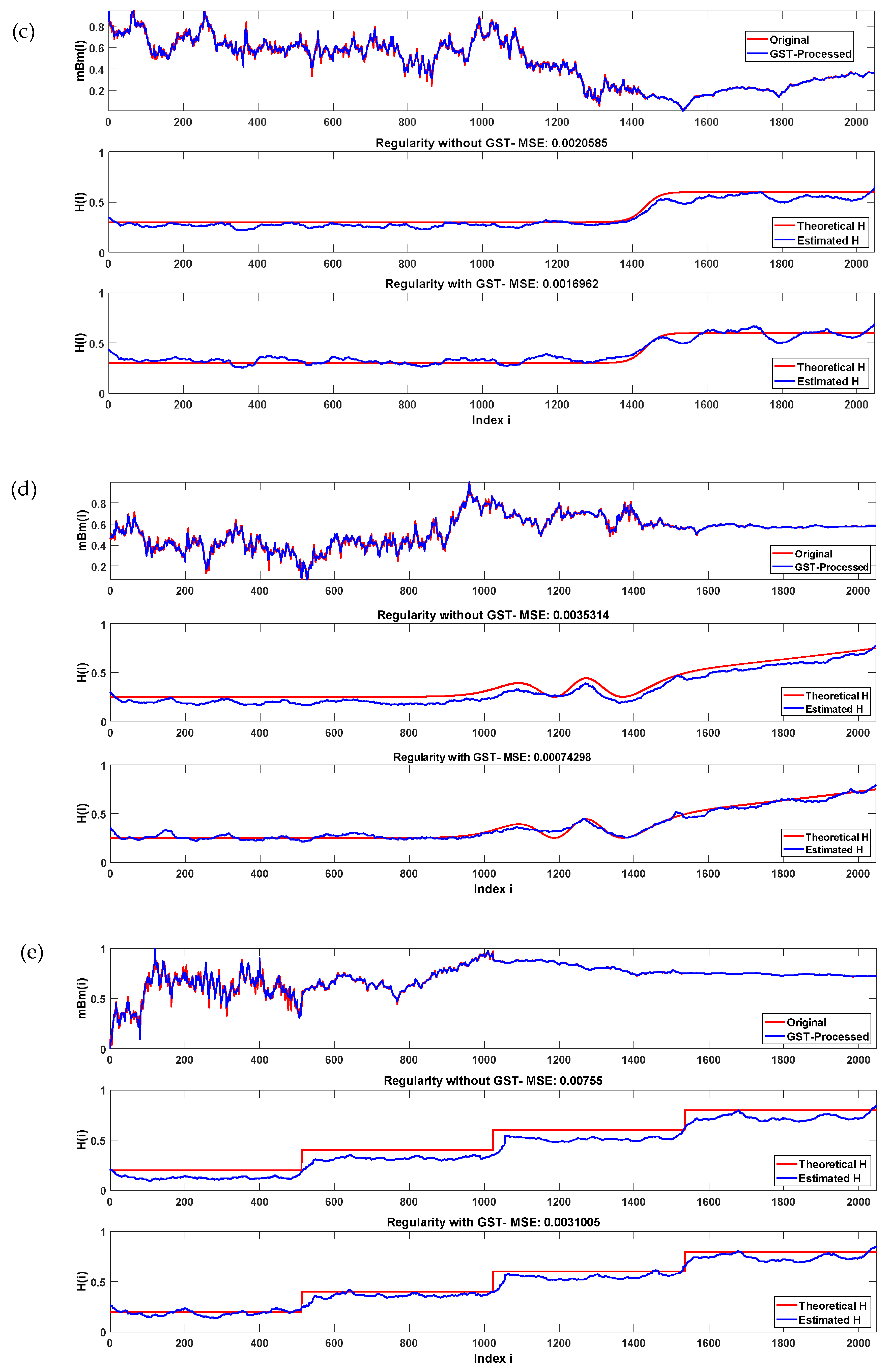
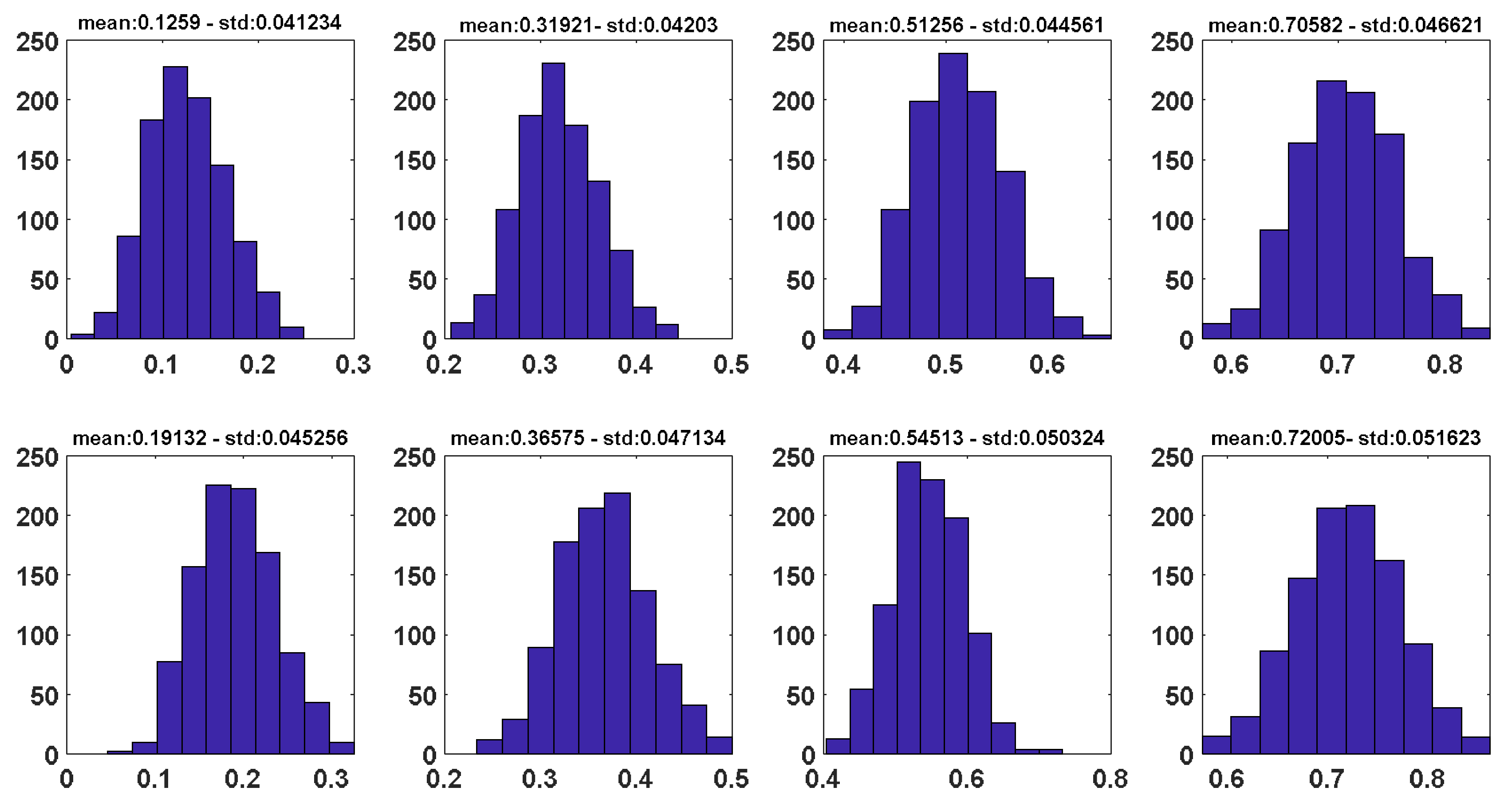
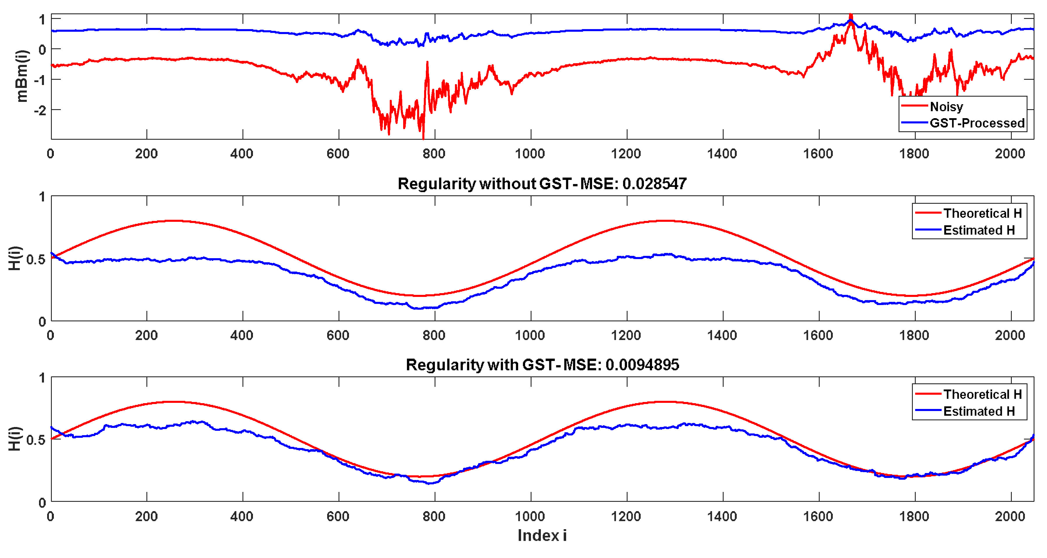
3. Application to Simulated Data

First, the grey system technique is implemented on simulated sonic logs data. These logs are considered as multifractional Brownian motions (mBms) simulated using the procedure proposed by Peltier and Lévy-Véhel [1]. The idea consists of generating N fractional Brownian motions (fBms) B_H(i) with the Hurst parameters $H\left(i\right),i=1,\dots ,N$, and then constructing the mBm path W_H(i) by setting

$$W_{H\left(i\right)}\left(i\right)=B_{H\left(i\right)}\left(i\right),i=1,\dots ,N.$$

(12)

In our applications, the fBms are simulated using the successive random additions (SRA) algorithm [34].

Five types of Hölder functions, linear $H_1$, periodic $H_2$, logistic $H_3,$synthetic $H_4$, and stairs $H_5$, are used to create $\mathrm{mBm}$ paths. They are defined as follows:

$$\begin{array}{c}{H}_1\left(t\right)=0.2+0.6t,\hfill \\ H_2\left(t\right)=0.5+0.3sin\left(4\pi t\right),\hfill \\ H_3\left(t\right)=0.3+\frac{0.3}{1+e^{-100\left(t-7\right)}} ,\hfill \\ H_4\left(t\right)=0.25+0.25t^2{\displaystyle (}1-cos\left(\frac{5\pi }{1+e^{-20\left(t-0.6\right)}}\right){\displaystyle )},\hfill \end{array}$$

$$H_5\left(t\right)=\{\begin{array}{c}0.2, i=1,\dots ,\frac{N}{4}\\ 0.4, i=\frac{N}{4}+1,\dots ,\frac{N}{2}\\ 0.6, i=\frac{N}{2}+1,\dots ,\frac{3N}{2}\\ 0.8, i=\frac{3N}{2}+1,\dots ,N\end{array} , t=\frac{i-1}{N}$$

In the following, for each type of regularity, a local Hölder function is computed, using the algorithm detailed in Section 2.3, from the raw mBm path and the mBm path processed by the GST theory. The obtained results are presented in Figure 1. As it can be noted, the mean square error (MSE) corresponding to the raw standardized mBm is larger than that related to the mBm path processed by GST.

Then, the convergence of the suggested algorithm is evaluated on the basis of 1000 realizations of the mBm paths created using the Hölder function H₅. Histograms of Hölder exponent values derived from the standardized raw mBm path (first line) and the mBm path processed by GST (second line) are illustrated in Figure 2. The first, second, third, and fourth columns are related to fixed positions whose indexes are i = N/8, 3N/8, 5N/8, and 7N/8 (N = 2048) which correspond to the theoretical Hölder exponent values: 0.2, 0.4, 0.6, and 0.8, respectively. It can be seen that the resulted histograms approximately follow a Gaussian distribution with small values of standard deviations. Note also that, for a given position, the mean of the Hölder exponent values derived from the mBm paths processed with the GST are closer to the theoretical H values than those which resulted in the standardized raw mBm paths. That confirms, again, the accuracy of the suggested method for the estimation of the local regularity functions.

The sensitivity of the proposed technique to noise level is demonstrated on simulated mBm paths. Here, the theoretical Hölder function considered in simulating mBm paths is a staircase (piecewise) function with nine pieces (stairs) presenting H values from 0.1 to 0.9 with an increment of 0.1. In each piece (stair), a fixed position is chosen on the simulated mBm path.

One thousand realizations of random noise are performed. For each realization, amounts of random noise are added to the noise-free mBm path to give signal-to-noise ratios (SNRs) of different values. In the following, SNR is defined as the ratio of signal power to the noise power (expressed in decibels).

For a given realization, the noisy mBm path is processed using GST. Then, the local H(t) is computed for both noisy and GST-processed mBm paths.

For a fixed SNR value, the H mean values of the noisy and GST-processed mBm paths at the nine fixed positions on mBm paths are obtained by averaging, over the total realizations number, the H values of regularity functions obtained from these mBm paths, respectively, at these positions.

From Figure 3, it can be noted that, for all of the fixed positions associated with different theoretical H values (varying from 0.1 to 0.9), the GST-based method enhances the accuracy of the estimated regularity of the noisy mBm paths for all the considered noise levels. As expected, for all of the considered positions, the Hmean values of the GST-processed mBm paths are increasingly closer to the corresponding theoretical H value as SNR reaches high values.

For illustration, an application of the proposed method to a realization of an mBm path, simulated with a periodic function, is presented in Figure 4. As can be noted, the function H(t) estimated using GST is more accurate than that obtained from the noisy mBm path, and presents the least error estimation value.

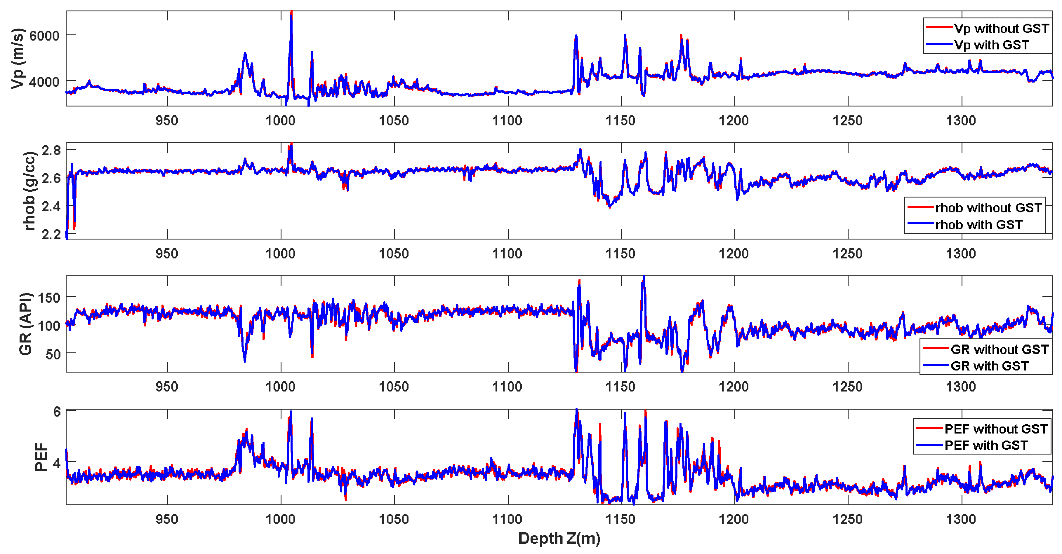
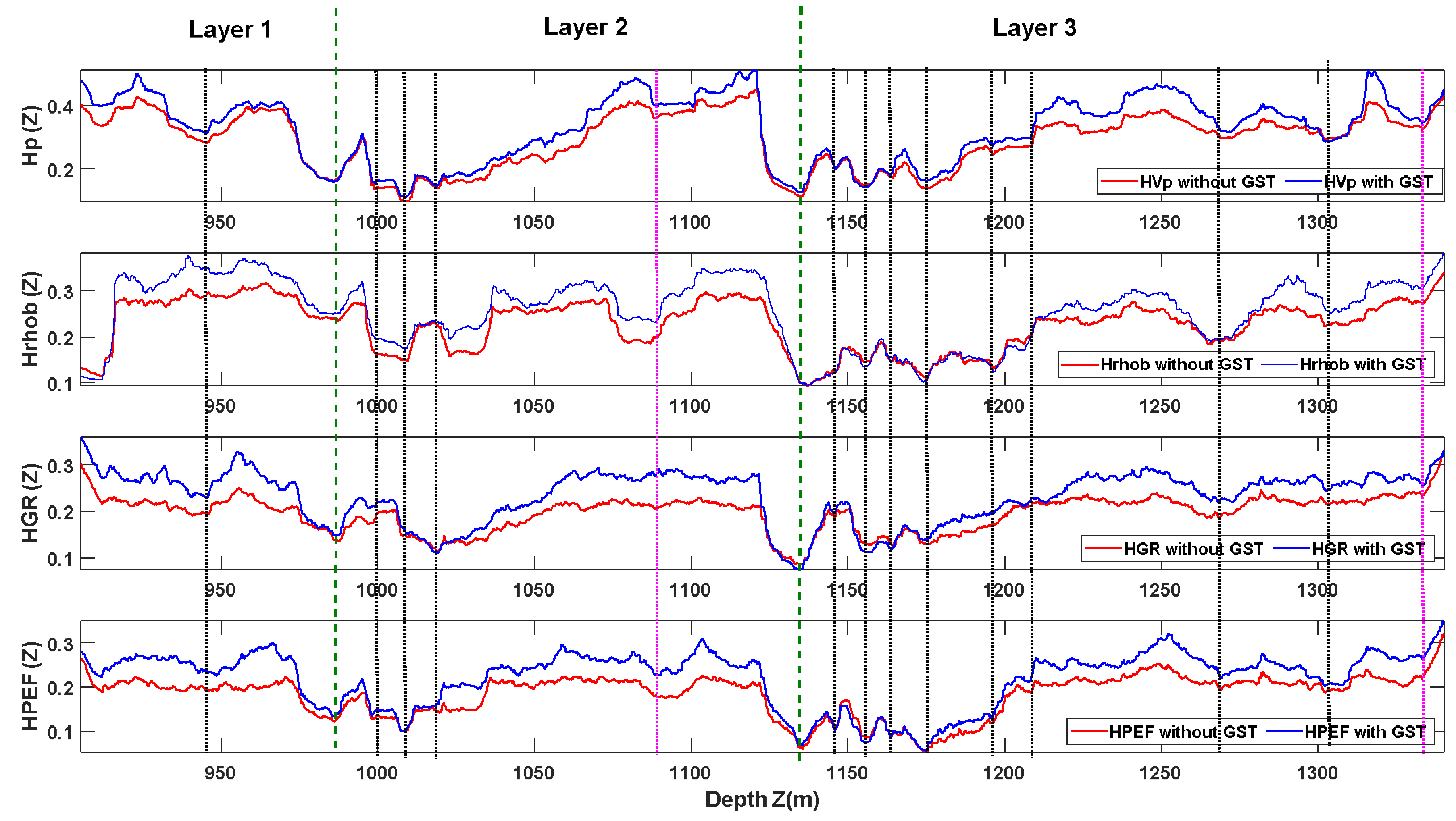
4. Application to Algerian Well Log Data

In this section, the aforementioned technique is implemented on well log data recorded in an Algerian exploration well located in southwestern Algeria. The analyzed logs are P-wave seismic velocity (Vp, m/s), bulk density (rhob, g/cm³), gamma ray (GR, API), and photoelectric absorption factor (PEF). The sampling depth of all the measurements is 0.1524 m.

From a lithological point of view, the investigated depth interval (905.256–1340 m) covers the lower Devonian reservoir is described as follows [35]:

• Layer L1 (905–981 m): shale.
• Layer L2 (981–1133 m): alternation of sandstone and shale, with limestone layers.
• Layer L3 (1133–1340 m): sandstone.

Figure 5 presents the raw and the GST-processed log data. The local Hölder exponent logs from well logs are calculated using the algorithms detailed in Section 2, from the raw data (in red) and data processed by the GST (in blue) (Figure 6). As can be observed, the lithological discontinuities, which are either layer boundaries or thin rock beds occurring within the studied depth intervals, are marked on the regularity profiles by sudden variations of H value.

Note, also, that the regularity logs computed using GST are more precise than those obtained from the raw logs, and lead to a more accurate lithological segmentation.

In addition, the correlation coefficients between the computed regularity logs are increased after application of GST on the investigated well logs (

Table 1. Correlation coefficients between the regularity profiles derived from the analyzed well logs (without GST | with GST).

	HVp	HGR	Hrhob	HPEF
HVp	1.00|1.00	0.84|0.88	0.61|0.65	0.80|0.84
HGR		1.00|1.00	0.57|0.62	0.73|0.76
Hrhob			1.00|1.00	0.83|0.84
HPEF				1.00|1.00

).

It can be noted that on the regularity profiles derived from the “porosity-dependent” logs, almost all the lithological discontinuities, which are either layer boundaries or thin rock beds occurring within the studied depth intervals, are marked by jumps in H value.

It is worthy to underline that for Vs log, the H logs obtained by both regularity estimation techniques (without and with GST) are matching across the studied depth intervals except for 700–900 m, 1650–1750 m, 2100–2200 m, 2650–2750 m, and 3050–3200 m. However, for Vp log, the regularity log obtained by the velocity log processed by GST presents relatively similar H values to those derived from the raw velocity data across almost all the investigated depth range, except within the depth interval of 2100–2200 m. The obtained results show that the GST allows to highlight local heterogeneities that cannot be seen from the regularity logs estimated from the raw velocity logs. Therefore, the regularity estimation obtained from the velocity well logs processed by the GST is more reliable than that yielded from the raw log data.

5. Conclusions

This study presents a new approach for accurately estimating Hölderian regularity using grey system theory (GST). The application on synthetic logs with different Hölder functions, simulated by the SRA method, shows that the regularity estimated from logs processed by the GST is more precise than that derived from the raw logs, even in the presence of noise. In addition, the suggested technique was implemented on Algerian exploration well log data. The estimated Hölder exponent logs allowed us to perform a lithological segmentation.

References

1. Peltier, R.F.; Lévy-Véhel, J. Multifractional Brownian Motion: Definition and preliminary results. Tech. Rep. INRIA RR 1995, 1, 2645. [Google Scholar]
2. Bicego, M.; Trudda, A. 2D shape classification using multifractional brownian motion. Lect. Notes Comput. Sci. 2010, 5342, 906–916. [Google Scholar]
3. Li, M.; Lim, S.C.; Hu, B.-J.; Feng, H. Towards describing multi-fractality of traffic using local Hurst function. Lect. Notes Comput. Sci. 2007, 4488, 1012–1020. [Google Scholar]
4. Silva, M.; Rocha, F.G. Traffic modeling for communications networks: A multifractal approach based on few parameters. J. Frankl. Inst. 2021, 358, 2161–2177. [Google Scholar] [CrossRef]
5. Wanliss, J. Fractal properties of SYM-H during quiet and active times. J. Geophys. Res. 2005, 110, 12. [Google Scholar] [CrossRef]
6. Wanliss, J.A.; Cersosimo, D.O. Scaling properties of high latitude magnetic field data during different magnetospheric conditions. Int. Conf. Substorms 2006, 8, 325–329. [Google Scholar]
7. Cersosimo, D.O.; Wanliss, J.A. Initial studies of high latitude magnetic field data during different magnetospheric conditions. Earth Planets Space 2007, 59, 39–43. [Google Scholar] [CrossRef] [Green Version]
8. Gaci, S.; Zaourar, N. A new approach for the investigation of the local regularity of borehole wire-line logs. J. Hydrocarb. Mines Environ. Res. 2010, 1, 6–13. [Google Scholar]
9. Gaci, S.; Zaourar, N.; Hamoudi, M.; Holschneider, M. Local regularity analysis of strata heterogeneities from sonic logs. Nonlin. Process. Geophys. 2010, 17, 455–466. [Google Scholar] [CrossRef] [Green Version]
10. Gaci, S.; Zaourar, N. Heterogeneities characterization from velocity logs using multifractional Brownian motion. Arab. J. Geosci. 2011, 4, 535–541. [Google Scholar] [CrossRef]
11. Gaci, S.; Zaourar, N. Two-Dimensional Multifractional Brownian Motion—Based Investigation of Heterogeneities from a Core Image. In Advances in Data, Methods, Models and Their Applications in Geoscience; InTech Ed.: London, UK, 2011. [Google Scholar]
12. Gaci, S.; Zaourar, N.; Briqueu, L.; Hamoudi, M. Regularity Analysis of Airborne Natural Gamma Ray Data Measured in the Hoggar Area (Algeria). In Advances in Data, Methods, Models and Their Applications in Geoscience; InTech Ed.: London, UK, 2011. [Google Scholar]
13. Gaci, S.; Zaourar, N.; Briqueu, L.; Holschneider, M. Regularity analysis applied to sonic logs data: A case study from KTB borehole site. Arab. J. Geosci. 2011, 4, 221–227. [Google Scholar] [CrossRef]
14. Deng, J. Control problems of grey system. Syst. Control. Lett. 1982, 1, 288–294. [Google Scholar]
15. Deng, J.L. The Primary Methods of Grey System Theory; Huazhong Institute of Technology Press: Wuhan, China, 1987; pp. 1–20. [Google Scholar]
16. Deng, J.L. Grey Theory; Huangzhong University of Science and Technology Press: Wuhan, China, 2002; pp. 1–15. [Google Scholar]
17. Liu, S.F.; Lin, Y. Grey Systems: Theory and Application; Springer: London, UK, 2006; pp. 1–78. [Google Scholar]
18. Wu, H.; Dong, Y.; Shi, W.; Clarke, K.C.; Miao, Z.; Zhang, J.; Chen, X. An improved fractal prediction model for forecasting mine slope deformation using GM (1, 1). Struct. Health Monit. 2015, 14, 502–512. [Google Scholar] [CrossRef] [Green Version]
19. Huang, Y.; Geng, J.; Guo, T. New seismic attribute: Fractal scaling exponent based on gray detrended fluctuation analysis. Appl. Geophys. 2015, 12, 343–352. [Google Scholar] [CrossRef]
20. Chen, X.; Li, J.; Han, H.; Ying, Y. Improving the signal subtle feature extraction performance based on dual improved fractal box dimension eigenvectors. R. Soc. Open Sci. 2018, 5, 180087. [Google Scholar] [CrossRef] [Green Version]
21. Zhang, Z.; Li, Y.; Qi, L. Research on multifractal dimension and improved gray relation theory for intelligent satellite signal recognition. Wirel. Netw. 2019, 1–9. [Google Scholar] [CrossRef] [Green Version]
22. Honório, B.; Drummond, R.; Vidal, A.; Sanchetta, A.; Leite, E. Well log denoising and geological enhancement based on discrete wavelet transform and hybrid thresholding. Energy Explor. Exploit. 2012, 30, 417–433. [Google Scholar] [CrossRef] [Green Version]
23. Fedi, M.; Fiore, D.; La Manna, M. Regularity Analysis Applied to Well Log Data. In Fractal Behaviour of the Earth System; Springer: Berlin/Heidelberg, Germany, 2005; pp. 63–82. [Google Scholar]
24. Khan, M.M.; Ahmad Fadzil, M.H. Singularity spectrum analysis of windowed seismograms. In Proceedings of the 8th International Conference on Frontiers of Information Technology—FIT ’10, Islamabad, Pakistan, 21–23 December 2010. [Google Scholar] [CrossRef]
25. Subhakar, D.; Chandrasekhar, E. Reservoir characterization using multifractal detrended fluctuation analysis of geophysical well-log data. Phys. A Stat. Mech. Its Appl. 2016, 445, 57–65. [Google Scholar] [CrossRef]
26. Partovi, S.M.A.; Sadeghnejad, S. Fractal parameters and well-logs investigation using automated well-to-well correlation. Comput. Geosci. 2017, 103, 59–69. [Google Scholar] [CrossRef]
27. Amoura, S.; Gaci, S.; Bounif, M.; Boussa, L. On characterizing heterogeneities from velocity logs using Hölderian regularity analysis: A case study from Algerian tight Devonian reservoirs. J. Appl. Geophys. 2019, 170. [Google Scholar] [CrossRef]
28. Prajapati, R.; Singh, U.K. Delineation of stratigraphic pattern using combined application of wavelet-Fourier transform and fractal dimension: A case study over Cambay Basin, India. Mar. Pet. Geol. 2020, 120, 104562. [Google Scholar] [CrossRef]
29. Boulassel, A.; Zaourar, N.; Gaci, S.; Boudella, A. A new multifractal analysis-based for identifying the reservoir fluid nature. J. Appl. Geophys. 2021, 185, 104185. [Google Scholar] [CrossRef]
30. Benassi, A.; Jaffard, S.; Roux, D. Gaussian processes and pseudodifferential elliptic operators. Rev. Mat. Iberoam. 1997, 13, 19–81. [Google Scholar] [CrossRef] [Green Version]
31. Ayache, A.; Taqqu, M.S. Multifractional process with random exponent. Publ. Mat. 2005, 49, 459–486. [Google Scholar] [CrossRef] [Green Version]
32. Ayache, A.; Jaffard, S.; Taqqu, M.S. Wavelet construction of generalized multifractional processes. Rev. Mat. Iberoam. 2007, 23, 327–370. [Google Scholar] [CrossRef] [Green Version]
33. Peltier, R.F.; Lévy-Véhel, J. A new method for estimating the parameter of fractional brownian motion. Tech. Rep. INRIA 1994, 1, 2396. [Google Scholar]
34. Turcotte, D.L. Fractals and Chaos in Geology and Geophysics; Cambridge University Press: Cambridge, UK, 1997; p. 398. [Google Scholar]
35. Sonatrach. Internal Technical Report of Southwestern Algeria Exploration Assets; Internal Publisher: Boumerdes, Algeria, 2007; p. 100. [Google Scholar]
Figure 1. Results obtained from mBm paths simulated with five types of Hölder function H(t): (a) linear; (b) periodic; (c) logistic; (d) synthetic; (e) stairs. Each figure consists of three panels, described as follows. The first panel represents the simulated mBm paths: standardized (in red) and processed by GST (in blue), the second panel shows the local Hölder exponent function estimated from the standardized mBm path (blue line) and the theoretical Hölder function (red line), and the third panel illustrates the local Hölder exponent function estimated from the mBm path processed by GST (blue line) and the theoretical Hölder function (red line).
Fractalfract 05 00086 g001aFractalfract 05 00086 g001b
Figure 2. Histograms of Hölder exponent values obtained from the standardized raw mBm path (1st line) and the mBm path processed by GST (2nd line). The histograms are resulted from 1000 realizations of mBm paths simulated with a stair-type Hölder function. The 1st, 2nd, 3rd, and 4th lines correspond to fixed positions i = N/8, 3N/8, 5N/8, and7N/8, whose theoretical Hölder exponent values are 0.2, 0.4, 0.6, and 0.8, respectively.
Fractalfract 05 00086 g002
Figure 3. Estimated Hmean value versus SNR value at the nine fixed positions, obtained from noisy mBm paths (in red) and GST-processed mBm paths (in blue). The Hmean values are obtained by averaging H values at the fixed positions resulted from 1000 realizations of mBm paths.
Fractalfract 05 00086 g003
Figure 4. Results obtained from a realization of mBm path simulated with a periodic Hölder function H(t) (SNR = 40). This figure consists of three panels, described as follows. The first panel presents the noisy mBm paths (in red) and the standardized and processed by GST (in blue), the second panel shows the local Hölder exponent function estimated from the noisy mBm path (blue line) and the theoretical Hölder function (red line), and the third panel illustrates the local Hölder exponent function estimated from the mBm path processed by GST (blue line) and the theoretical Hölder function (red line).
Fractalfract 05 00086 g004
Figure 5. Physical properties measured within the depth interval (905–1340 m) in borehole W1: the raw data (in red) and the data processed by the GST (in blue) [35].
Fractalfract 05 00086 g005
Figure 6. Regularity profiles obtained from the physical measurements of Figure 5. Dashed lines: layer boundaries (in green), limestone beds (in black), and shale beds (in magenta) (the layer boundaries in dashed lines are taken from [35]). The H logs are computed using the algorithm detailed in Section 2.3, from the raw data (in red) and data processed by the GST (in blue). Note that the local extrema of the H logs correspond to the lithological discontinuities.
Fractalfract 05 00086 g006