1. Introduction
In this paper, we will develop a multigrid method to numerically solve, highly efficiently, the tempered fractional diffusion equation. Multigrid is known to be an efficient and powerful numerical technique, particularly, for solving elliptic partial differential equations (PDEs). The convergence rate is usually independent of the mesh size [
1,
2]. Different methodological enhancements have been considered to generalize the range of applicability of the multigrid method, such as nontrivial smoothing methods, for example, in [
3,
4], coarsening and interpolation, like in [
5,
6], convection dominated problems [
7], and so on, each time enlarging the range of robust and efficient multigrid applications, see also [
8].
Recently, multigrid methods have also been applied to solving fractional diffusion equations (FDE) in the literature [
9,
10,
11,
12,
13]. Fractional diffusion equations are governed by their long range interactions, so that, after discretization, full matrices result. These full matrices may possess a favorable structure, like a Toeplitz matrix structure, which is beneficial regarding efficient matrix-vector multiplication. Pang and Sun [
9], for example, developed multigrid methods where the coarse grid operator retained the Toeplitz-like structure, by means of the Meerschaet–Tadjeran method. Hamid et al. constructed multigrid methods for a two-dimensional FDE problem, which was discretized by means of a CN-WSGD scheme, and they confirmed that multigrid methods performed better than classical preconditioners based on multilevel circulant matrices, in [
13]. Gu, et al. [
14] reformulated the classical time-stepping schemes as a kind of parallel-in-time (PinT) methods for both one- and two-dimensional space fractional diffusion equations and the fast Krylov subspace method with tau preconditioners is used to solve the resulting discretized linear systems.
It is well-known that a fractional derivative can be employed to accurately describe memory properties and hereditary effects of materials and processes. Differential equations with fractional operators are nowadays commonly applied in different fields of science and engineering, for example, in physics [
15,
16,
17,
18], hydrology [
19,
20,
21,
22], biology [
23,
24], or even finance [
25,
26,
27,
28]. Fractional derivatives also have a natural application when studying anomalous diffusion (for an extensive review, we refer to [
29]). In another setting, Lévy flight models are used to mathematically describe the super-diffusion phenomenon, whose jumps have infinite moments in complex systems. So-called tempered fractional operators were introduced to describe probability density functions related to the positions of particles, by applying an exponential tempering of the probability of large jumps occurring in these Lévy flights [
30]. These tempered derivatives have applications in physics [
31,
32,
33], ground water hydrology [
34], and even in finance [
35,
36].
A recent significant research effort on discretization methods for differential equations with tempered fractional derivatives has resulted in accurate finite element techniques [
37], finite differences [
31,
33,
38], and also spectral methods [
32,
39,
40]. For example, Cartea and Del-Castillo-Negrete [
35] defined a finite difference scheme to price exotic options under Lévy processes. Zhang et al. [
36] presented a second-order discretization for the tempered fractional Black–Scholes equation and analyzed the stability and convergence properties of it. Li and Deng [
31] defined higher-order discretizations based on a weighted and shifted Grünwald type approximation for the tempered fractional derivative. They also provided stability and convergence results for a second-order discretization of the tempered fractional diffusion equation. Zhao et al. [
41] designed the first-order fully implicit and semi-implicit schemes for the nonlinear tempered fractional diffusion equation with variable coefficients, where the stabilities and convergences of the two numerical schemes are proved under several assumptions. Then the PinT implementation of the fully implicit scheme is given and the resulting nonlinear system is solved by using the fast preconditioned iterative method.
In [
42], we developed the third-order discretizations based on the weighted and shifted Grünwald type difference (WSGD) for the tempered fractional derivatives. We also analyzed the stability and convergence properties for the tempered fractional diffusion equation, and proved that the third-order accurate scheme is unconditionally stable for a large ranges of problem parameters. A third-order scheme for the tempered Black–Scholes equation is also proposed and tested numerically. In this paper, we focus on the multigrid solution method for the tempered fractional diffusion and the fractional Black–Scholes equation, discretized by means of the second and third order CN-WSGD schemes we proposed before. Numerical results confirm that the proposed method is accurate and efficient.
The paper is organized as follows. In
Section 2, we will provide the discretization details for the tempered fractional diffusion equation.
Section 3.1 and
Section 3.2 describe the components of the multigrid method for the second-order and the third-order discrete schemes for the fractional diffusion equation. A contribution of this paper is the multigrid convergence analysis for these discrete schemes in this section. In
Section 4, we then present some numerical results to confirm the accuracy and efficiency of the proposed methods. Moreover, we also solve the fractional Black–Scholes equation in this section. Finally, we summarize our findings in the last section.
2. Numerical Schemes for the Tempered Fractional Diffusion Equation
We consider the following tempered fractional diffusion equation
where
,
is the source term,
with
,
and
The Riemann–Liouville tempered fractional derivatives, that we encounter in this equation, are defined as follows.
Definition 1 (See [31]).For , let be -times continuously differentiable on with its nth derivative integrable on any subinterval of , and Then, the left Riemann–Liouville tempered fractional derivative of order α is defined asthe right Riemann–Liouville tempered fractional derivative of order α is defined aswhere ’a’ and ’b’ can be extended to and ∞, respectively. We will construct a high-order scheme based on the tempered-WSGD operators for the tempered fractional derivative in space. The following results are developed for the tempered fractional operators in [
31,
42].
Remark 1. In this paper, we consider a well-defined function on a bounded interval , and the function will be zero extended for or , so that , and , and their Fourier transforms belong to . The α-th order left and right Riemann–Liouville tempered fractional derivatives of at grid point x can then be approximated by tempered-WSGD operators and , as followssee [31,42] for details. The second- and third-order operators are given in Section 2.1 and Section 2.2. Let the equidistant time partition,
, and spatial grid,
, be defined, where
and
. Using the high-order tempered-WSGD operators
and
(as explained in Remark 1), high-order scheme for the first-order spatial derivative with
, and a Crank–Nicolson discretization in time, the numerical scheme for (
1) reads
where
represents the solution of (
1) at the point
and
Rewriting gives us
Denote by
the solution of the numerical scheme for (
1) at point
. The numerical scheme can now be written as
We will use the following notations, for vector
. Further,
,
,
, and
The corresponding matrix form of (
6) then reads
where
and
2.1. Second-Order Discrete Scheme for the Tempered Fractional Diffusion Equation
We first present the second-order scheme for the tempered fractional diffusion Equation (
1). Here, the second-order operators are defined as follows,
where
with
satisfying the following conditions,
and the weights
are given by
We will present the second-order scheme for the tempered fractional diffusion equation in detail here. Using the tempered-WSGD operators,
and
for the tempered fractional derivatives, and the second-order scheme for the first-order spatial derivative, the numerical scheme can now be written as,
The corresponding matrix form of (
16) then reads
with
,
as defined in (
9), (
11) when
,
,
and
The stability and convergence of the second-order scheme for the tempered fractional diffusion Equation (
1), when
and
are constants have already been presented in [
31]. In a similar way, we can derive and prove the following theorem, based on the lemma below.
Lemma 1 (From [31]).For and , ifthen the weight coefficients and satisfy the following properties, - 1.
, , ,
- 2.
,
- 3.
, ,
Theorem 1. For , and , if , the numerical scheme (16) is stable forandDenoting and , moreover, it is found that 2.2. Third-Order Discrete Scheme for the Tempered Fractional Diffusion Equation
In this work, we also consider the third-order operators. They are defined as
and
where
with
satisfying the following conditions
The weights,
are found to be
Using the tempered-WSGD operators,
and
, for the tempered fractional derivatives, and the fourth-order scheme for the first-order spatial derivative, we find the following numerical discretization for (
1)
The matrix form now looks as follows
with
as defined in (
9), (
11) with
,
and
with
We have already discussed the stability and convergence of the third-order scheme for the tempered fractional diffusion Equation (
1) when
and
are constants in the paper [
42]. Before we introduce the stability and convergence of the third-order scheme (
25), we define the functions
and the generating function,
We obtain the stability for the numerical scheme (
25), based on the theorem below.
Lemma 2 (From [42]).Let the matrices and be given via the numerical scheme (7). For and , if we can find (analytically, or with the help of numerical techniques) values of for which the generating functions of are negative, then the eigenvalues of the matrix are negative too. In a similar way as in [
42], we have the following theorem.
Theorem 2. If, for , the generating functions given in (31), are negative, the numerical scheme (25) is stable. Theorem 3. Assuming function to be the solution of Equation (1) on a bounded interval , which can be zero extended for or , so that , and and its Fourier transform also belong to . Let’s denote by and . With solutions and of Equations (5) when and (25), respectively, we have, for , if , , It is our aim in this paper to solve the resulting discrete equations by means of a multigrid technique. The challenge here is, of course, the occurance of the nonlocality of these discretization schemes for the tempered fractional derivatives.
3. Multigrid Method for Tempered Fractional Diffusion Equation
In this subsection, we provide a multigrid method (see, for example in [
8]) to solve the presented linear systems originating from the discretized fractional diffusion equations. Actually, the classical multigrid setting will be employed here, based on the direct coarse grid discretization. The corresponding two-grid algorithmic description is the following:
- 1.
Pre-smoothing:
Compute
by applying
steps of a smoothing procedure to
- 2.
Coarse-grid correction:
Define the residual: ,
Restrict the residual (fine-to-coarse grid transfer): ,
Solve ,
Interpolate the correction (coarse-to-fine grid transfer): ,
Compute a new approximation: .
- 3.
Post-smoothing:
Compute
by applying
steps of a smoothing procedure to
For the above description, the notation is as follows:
denote the number of smoothing steps. We will use .
The classical fine-to-coarse restriction operator
is employed,
The scaled transpose of the restriction is the coarse-to-fine interpolation operator, i.e., .
The fine grid operator
and the coarse grid operator
are defined as in Equations (
18) or (
28). Obviously, the coefficient matrix possess the Toeplitz-like structure.
The recursive generalization of this classical two-grid scheme towards multiple grids is well-known.
For the tempered fractional diffusion equation, we will be using the damped Jacobi iteration as the smoother. Here we use
Then
We can easily generalize the classical Jacobi iteration by introducing a relaxation parameter
, in the standard way, i.e.,
where
represents the main diagonal of matrix
. The smoother then becomes,
Remark 2. For general full matrices, a matrix-vector multiplication is an expensive task. However, in the present context with the fractional diffusion equations, we can benefit from the choices made within the discretization and regarding the multigrid components. The overall computational complexity of the multigrid method here is therefore O() at each time step, despite the fact that we’re dealing with a full matrix. In this paper, the resulting coefficient matrix which contains three Toeplitz matrices possesses a Toeplitz-like structure. It is however nontrivial to use fast Toeplitz solvers directly when the coefficients would depend on the spatial position, i.e., .
3.1. Multigrid Convergence Analysis for Second-Order Tempered Fractional Diffusion Scheme
Here, we will analyze the convergence of the multigrid method for the second-order discrete scheme. To simplify the analysis, we assume that
. Then we have
. We denote by
with
. Then, we find that
is a symmetric Toeplitz matrix, of the following form,
where
.
We need the following lemmas regarding the properties of our matrix, in order to prove multigrid convergence.
Lemma 3 (From [31]).Using the notation, For , and , if , then the matrix,is diagonally dominant and all eigenvalues of are negative. Moreover, if a matrix is real-valued, symmetric, strictly diagonally dominant or irreducibly diagonally dominant, with positive diagonal entries, then it is positive [
31].
We have the following lemma regarding our matrix .
Lemma 4. For and , if , the matrix defined in (18) is diagonally dominant and all eigenvalues of are positive. Proof. From Lemma 1, we obtain,
Therefore, we have the following result for the
ith row of the matrix
It can seen that the matrix
is strictly diagonally dominant for
. From Lemma (3), we then conclude that
is a symmetric, positive definite matrix. □
We will use the following inner products,
Here is the Euclidean inner product.
Theorem 4 (From [43]).For a symmetric, positive definite matrix , suppose that the damping parameter ω, in the damped Jacobi smoother, in (36), is properly chosen, to fulfillwhere denotes the spectral radius of the matrix. Then, in (36) satisfies The inequality (
42) is the well-known smoothing property [
2]. We find that
, when
satisfies (
41). As
is symmetric, positive definite and diagonally dominant, we have
hence
Here we choose
which satisfies (
41).
For the two-grid method (TGM), the correction operator is given by
Therefore, the convergence factor of the TGM reads
. For convenience, we consider here the case that
and
.
Theorem 5 (From [43]).Let be symmetric and positive definite and let be chosen such that satisfies the smoothing condition (42), i.e.,Suppose that has full rank and that there exists a scalar , such thatThen, and the convergence factor of the TGM satisfies In other words, we just need to find a suitable
-value to satisfy (
46) and then we find that the convergence of TGM is independent of
N. Let
be the
one-dimensional discrete Laplacian matrix. Then
is also a symmetric positive definite Toeplitz matrix.
Lemma 5. For and , if , we denote . Then is symmetric positive definite.
Proof. Since both
and
are symmetric Toeplitz,
is also symmetric Toeplitz. We have
where
,
and
For the
k-th row, we then obtain that
Hence,
is strictly diagonally dominant, and we know that
is positive since
. □
From Lemma 5, it’s easy to see that
Now we are ready to provide the proof for the TGM convergence, in the following theorem.
Theorem 6. Suppose that is defined in (18) and such that satisfies the smoothing condition (42). The convergence factor of the TGM satisfies Proof. .
Let
. Then we have,
It suggests that
From Lemma 5, we obtain
To satisfy (
45), we here take
From Lemma 3, we have
Combining (
54) and (
55) with
, we have
, and
Based on Theorem 5, we obtain
□
Remark 3. It can be seen that the TGM converges linearly from Theorem 6 when is defined in (18) and . In fact, the TGM will also be stable when but satisfies . The numerical examples in Section 4 also show cases like this. 3.2. Multigrid Convergence for the Third-Order Tempered Fractional Diffusion Discretization
In this subsection, we will repeat the analysis of the multigrid convergence, but now for third-order accurate schemes for the tempered fractional diffusion equation.
To simplify the multigrid analysis of the third-order scheme, we assume
, and we denote by
with
. We then find that
is a symmetric Toeplitz matrix of the following form,
where
.
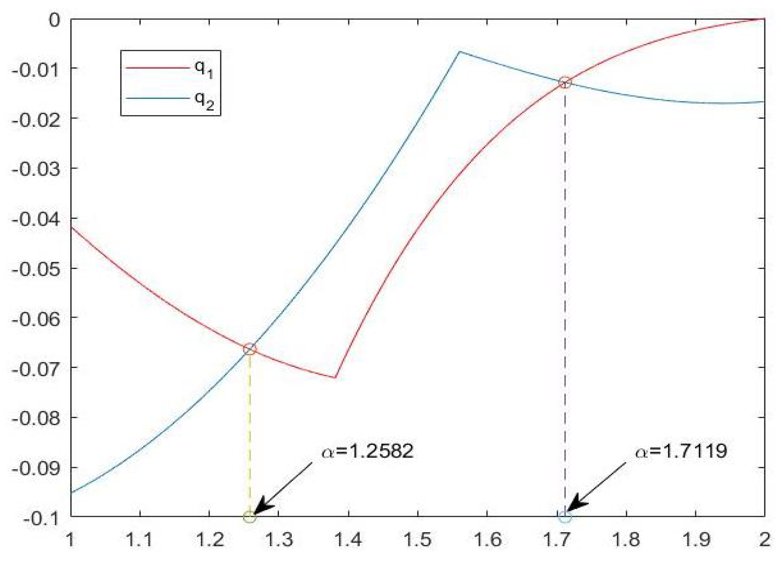
For
, we denote
and
where
.
The impact of varying
on
and
is graphically illustrated in
Figure 1. Particularly, it can be observed that when
,
and
.
Again, we will be looking into the matrix properties for the third-order discretization. For this, we will be using the following lemmas and theorems.
Theorem 7 (From [42]).For , and , the following properties are satisfied, Lemma 6 (From [42]).Let the matrices and be given by (7) when . For and , let be the generating function of . If , we have and is negative. For , we obtain the following result, which is similar to Lemma 1.
Lemma 7. For , , and , the matrix is diagonally dominant and all eigenvalues of are positive.
Proof. From Theorem 7, we obtain
Therefore, we find the following result for the
i-th row of matrix
It can seen that matrix
is strictly diagonally dominant, for
. From Lemma 3, we conclude that
is a symmetric, positive definite matrix. □
Using the same inner products as for the second-order case, i.e.,
with
the Euclidean inner product, and also using
, which satisfies (
41) for the third-order scheme (
25), we have, similar to Lemma 5, the following lemma
Lemma 8. For , we denote . Then is symmetric, positive definite, when .
We thus obtain the following theorem regarding the TGM convergence.
Theorem 8. Suppose that is defined as in (58) and such that satisfies the smoothing condition (42). The convergence factor of the TGM then satisfies Proof. The definition of
and
are the same as in Theorem 6, with
. We have the following result, which is similar to (
51)
This result suggests that
From Lemma 8, we obtain
To satisfy (
45), we will here use
With Lemma 6, we find
Combining (
67) and (
68), with
, gives us
, and,
Based on Theorem 5, we thus obtain
□
5. Conclusions
In this paper, we analyzed a classical multigrid method for second- and third-order numerical schemes for the tempered fractional diffusion equation. We have detailed the classical multigrid components, like the damped Jacobi smoothing iteration, and the direct coarse grid approximation, which is based on the second- and third-order discrete schemes. A focus of this paper was the multigrid convergence analysis, which was based on the properties of the occurring discretization matrices.
Moreover, we have also shown that the multigrid method converged very well for the tempered fractional Black–Scholes equation.
Obviously, the numerical schemes presented in this paper are computationally highly accurate and efficient.


