Comparison of Two Different Analytical Forms of Response for Fractional Oscillation Equation

Abstract

The impulse response of the fractional oscillation equation was investigated, where the damping term was characterized by means of the Riemann–Liouville fractional derivative with the order $\alpha$ satisfying $0\le \alpha \le 2$. Two different analytical forms of the response were obtained by using the two different methods of inverse Laplace transform. The first analytical form is a series composed of positive powers of t, which converges rapidly for a small t. The second form is a sum of a damped harmonic oscillation with negative exponential amplitude and a decayed function in the form of an infinite integral, where the infinite integral converges rapidly for a large t. Furthermore, the Gauss–Laguerre quadrature formula was used for numerical calculation of the infinite integral to generate an analytical approximation to the response. The asymptotic behaviours for a small t and large t were obtained from the two forms of response. The second form provides more details for the response and is applicable for a larger range of t. The results include that of the integer-order cases, $\alpha =$ 0, 1 and 2.

1. Introduction

From the middle of the last century, the theory of fractional calculus and its applications have attracted much attention and stimulated scholars’ interest. Currently, fractional calculus has been applied to different science and engineering fields to describe memory phenomena, intermediate processes, hereditary properties, and complex phenomena [1,2,3,4,5,6,7,8,9]. In particular, fractional calculus has been applied to the mathematical modelling of viscoelastic materials. For some viscoelastic materials, the stress–strain relation can be more accurately described by introducing fractional derivatives [3,4,5,10,11,12].

Scott-Blair [10] introduced the fractional derivative to characterize a viscoelastic body whose mechanical properties are intermediate between a pure elastic solid (Hooke model) and a pure viscous fluid (Newton model). Such a fractional element was called a spring-pot in [12] or the Scott-Blair model in [3]. If an oscillator connects with such viscoelastic material, then the resistance term may be built up resorting to the fractional derivative, called a fractional oscillator. In [13], relaxation, creep, dissipation, and hysteresis resulting from a six-parameter fractional constitutive model were considered.

Fractional oscillation was considered by Bagley and Torvik [14], Beyer and Kempfle [15], and others [16,17,18,19,20]. In [14], a fractional equation describing the in-plane oscillations of a rigid plate immersed in a Newtonian fluid was established. In [15], the uniqueness and causality for the solution of the fractional oscillation equation were explored with the help of the Fourier transformation and frequency domain analysis. Achar et al. [16] studied the fractional oscillation equation in the form of the fractional integral. We notice that the fractional oscillation equation considered in [16] is a two-term-equation without the second order derivative. In [17], oscillator equations derived from the relaxation kernel and the creep kernel were considered based on the fractional calculus Kelvin–Voight model, Maxwell model, and standard linear solid model, respectively. In [17,18,19], the Bromwich’s integral formula of inverse Laplace transform and the residue theorem were used for the solutions of fractional oscillation equations. In [20], three classes of fractional oscillators with the Weyl fractional derivative were investigated. In [21], the stability of the linear fractional oscillator with the Caputo fractional derivative was explored based on the stability switch. For detailed discussions of fractional oscillator systems and their applications, readers may refer to the recent monograph [9]. In [22], the viscous inertia described by the fractional derivative was reported. In [23,24], nonlinear oscillators were considered for their dynamical behaviour, resonance phenomena, bifurcation, and chaos. In [25], vibration theory with variable-order fractional forces was proposed.

Next, we recall the definitions of the involved fractional integral and derivative. For additional details, we refer the readers to [1,2,3,4,5,6]. Let $f(t)$ satisfy $f(t)=0$ for $t<0$ and be piecewise continuous on $(0,+\infty )$ and integrable on any finite subinterval of $(0,+\infty )$. Then, the Riemann–Liouville fractional integral of $f(t)$ of order $\nu >0$ is defined as the convolution

$$J_t^{\nu }f(t)=\frac{t^{\nu -1}}{\mathsf{\Gamma }(\nu )}\ast f(t)={\int }_0^t\frac{{(t-u)}^{\nu -1}}{\mathsf{\Gamma }(\nu )}f(u)du,t>0,$$

(1)

where $\mathsf{\Gamma }(·)$ is Euler’s gamma function. The Riemann–Liouville fractional derivative of order $\alpha$ ($m-1<\alpha <m$) is defined as a composition of the mth derivative and $(m-\alpha )$-order integral,

$$D_t^{\alpha }f(t)=\frac{d^m}{d{t}^m}\left(J_t^{m-\alpha }f(t)\right),t>0,m-1<\alpha <m,m\in {\mathbb{N}}^{+}.$$

(2)

Exchanging the order of the derivative and integral in Equation (2) leads to the definition of the Caputo fractional derivative. The Riemann–Liouville fractional derivative has weaker requirements for the function $f(t)$ than the Caputo fractional derivative. In this paper, the Riemann–Liouville fractional derivative is used to model the fractional oscillation. We use the Laplace transform

$$F(s)=\mathcal{L}[f(t)]={\int }_{0^{-}}^{+\infty }f(t)e^{-st}dt.$$

(3)

Then, the Laplace transform of the Riemann–Liouville fractional derivative is $\mathcal{L}\left[D_t^{\alpha }f(t)\right]=s^{\alpha }F(s).$

In this paper, by using two different methods of inversion Laplace transform, we consider the impulse response of the fractional oscillation equation

$$\begin{array}{cc}& m{x}^{″}(t)+c{D}_t^{\alpha }x(t)+kx(t)=\delta (t),m,c,k>0,\end{array}$$

(4)

where $\alpha$ satisfies $0\le \alpha \le 2$, $\delta (t)$ is the Dirac-$\delta$ function, and $x(t)\equiv 0$ when $t<0$. We note that in [11,14], the cases of $\alpha =1/2$ and $\alpha =3/2$ were introduced, respectively.

Applying the Laplace transform to Equation (4) leads to

$$m{s}^{2}X(s)+c{s}^{\alpha }X(s)+kX(s)=1.$$

Solving the transform function, we have

$$X(s)=\frac{1}{m{s}^2+c{s}^{\alpha }+k}.$$

(5)

For the integer-order case $\alpha =1$, using the Laplace transform table, we can obtain the response in three subcases, i.e., overdamping, criticaldamping, and underdamping:

$$x(t;\alpha =1)=\left\{\begin{array}{cc}\frac{2}{\sqrt{c^2-4mk}}{e}^{-\frac{c}{2m}t}sinh\left(\frac{\sqrt{c^2-4mk}}{2m}t\right),& c^2-4mk>0,\hfill \\ \frac{t}{m}{e}^{-\frac{c}{2m}t},& c^2-4mk=0,\hfill \\ \frac{2}{\sqrt{4mk-c^2}}{e}^{-\frac{c}{2m}t}sin\left(\frac{\sqrt{4mk-c^2}}{2m}t\right),& c^2-4mk<0.\hfill \end{array}\right.$$

(6)

We note that the three subcases correspond to the Laplace transform $X(s)$ having two real simple poles, one real second-order pole, and a pair of complex conjugate simple poles, respectively, in the s-plane.

For the integer-order cases $\alpha =0$ and $\alpha =2$, making use of the Laplace transform table, the responses are obtained as the periodic oscillations

$$\begin{array}{c}\hfill x(t;\alpha =0)=\frac{1}{\sqrt{m(k+c)}}sin\left(\sqrt{\frac{k+c}{m}}t\right),\end{array}$$

(7)

$$\begin{array}{c}\hfill x(t;\alpha =2)=\frac{1}{\sqrt{(m+c)k}}sin\left(\sqrt{\frac{k}{m+c}}t\right).\end{array}$$

(8)

Starting from Equation (5), we use two different methods of inverse Laplace transform to give two different forms of the response. One is in a series form constituted with positive powers of t and converges rapidly for small t, while another is the sum of a harmonic damped oscillation and a decayed function in the form of an infinite integral, where the infinite integral converges rapidly for a large t and is appropriately evaluated by using the Gauss–Laguerre quadrature formula. The text is organized as follows. In the next section, we present the response rapidly convergent for a small t. In Section 3, we derive the response rapidly convergent for a large t. Section 4 presents our conclusions.

2. Solution Rapidly Convergent for Small t

We decompose the right hand side of Equation (5) to a series of negative powers of s and then use the inversion method term by term. We will apply the expansion formula of power series twice, and such expansions work for such large $\mathrm{Re}(s)$ as specified below. The present method is based on that of the Green’s function for fractional differential equations [4].

First, we can rewrite $X(s)$ in the form

$$X(s)=\frac{1}{s^{\alpha }(m{s}^{2-\alpha }+c)\left(1+\frac{k{s}^{-\alpha }}{m{s}^{2-\alpha }+c}\right)},$$

(9)

and expand the right hand side as

$$\begin{array}{ccc}\hfill X(s)& =& \frac{1}{s^{\alpha }(m{s}^{2-\alpha }+c)}\sum _{j=0}^{+\infty }{(-1)}^j\frac{k^j{s}^{-\alpha j}}{{\left(m{s}^{2-\alpha }+c\right)}^j}.\hfill \end{array}$$

(10)

Sufficient conditions for the above expansion to hold are

$$\begin{array}{c}\hfill \mathrm{Re}(s)>max\left\{1,{\left(\frac{k+c}{m}\right)}^{\frac{1}{2-\alpha }}\right\}\mathrm{if}0\le \alpha <2\mathrm{and}\mathrm{Re}(s)>\sqrt{\frac{k}{m+c}}\mathrm{if}\alpha =2.\end{array}$$

(11)

Furthermore, we rewrite Equation (10) as

$$\begin{array}{ccc}\hfill X(s)& =& \sum _{j=0}^{+\infty }{(-1)}^j\frac{k^j}{m^{j+1}{s}^{2(j+1)}}{\left(1+\frac{c}{m{s}^{2-\alpha }}\right)}^{-(j+1)}.\hfill \end{array}$$

(12)

By using the formula

$${(1+z)}^{-n}=\sum _{l=0}^{+\infty }{(-1)}^l\frac{(n+l-1)!}{l!(n-1)!}{z}^l,|z|<1,n\ge 1,$$

(13)

expanding the right hand side of Equation (12) yields the series of negative powers of s,

$$X(s)=\sum _{j=0}^{+\infty }\frac{{(-k)}^j}{j!}\sum _{l=0}^{+\infty }\frac{{(-c)}^l}{l!}\frac{(j+l)!}{m^{j+l+1}}\frac{1}{s^{2(j+1)+(2-\alpha )l}},$$

(14)

where the expansion holds for s satisfying the conditions

$$\begin{array}{c}\hfill \mathrm{Re}(s)>{\left(\frac{c}{m}\right)}^{\frac{1}{2-\alpha }}\mathrm{if}0\le \alpha <2,\mathrm{and}c<m\mathrm{if}\alpha =2.\end{array}$$

(15)

Now, taking the inverse Laplace transform to Equation (14) term by term, we obtain the response in the series form constituted with positive powers of t,

$$x(t)=\sum _{j=0}^{+\infty }\frac{{(-k)}^j}{j!}\sum _{l=0}^{+\infty }\frac{{(-c)}^l}{l!}\frac{(j+l)!}{m^{j+l+1}}\frac{t^{2j+1+(2-\alpha )l}}{\mathsf{\Gamma }(2j+2+(2-\alpha )l)}.$$

(16)

By setting $n=j+l$, Equation (16) has the form

$$x(t)=\sum _{n=0}^{+\infty }\sum _{j=0}^n\frac{n!{(-k)}^j{(-c)}^{n-j}}{j!(n-j)!m^{n+1}}\frac{t^{2j+1+(2-\alpha )(n-j)}}{\mathsf{\Gamma }(2j+2+(2-\alpha )(n-j))}.$$

(17)

Here, the series converges rapidly for a small t, and the response has the asymptotic behaviour

$$x(t)\sim \frac{t}{m},t\to 0.$$

(18)

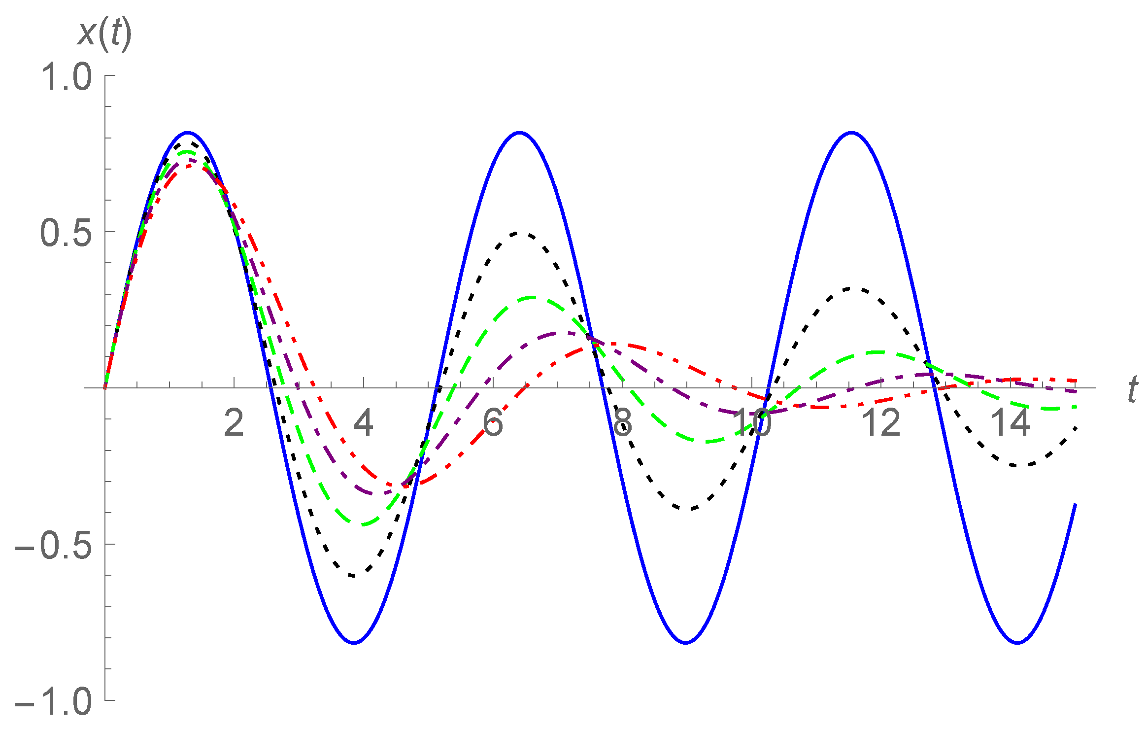
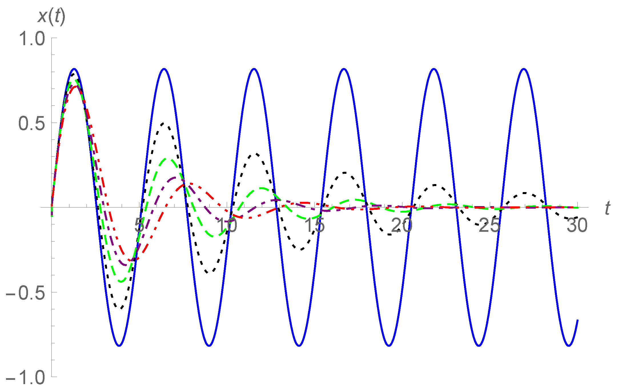
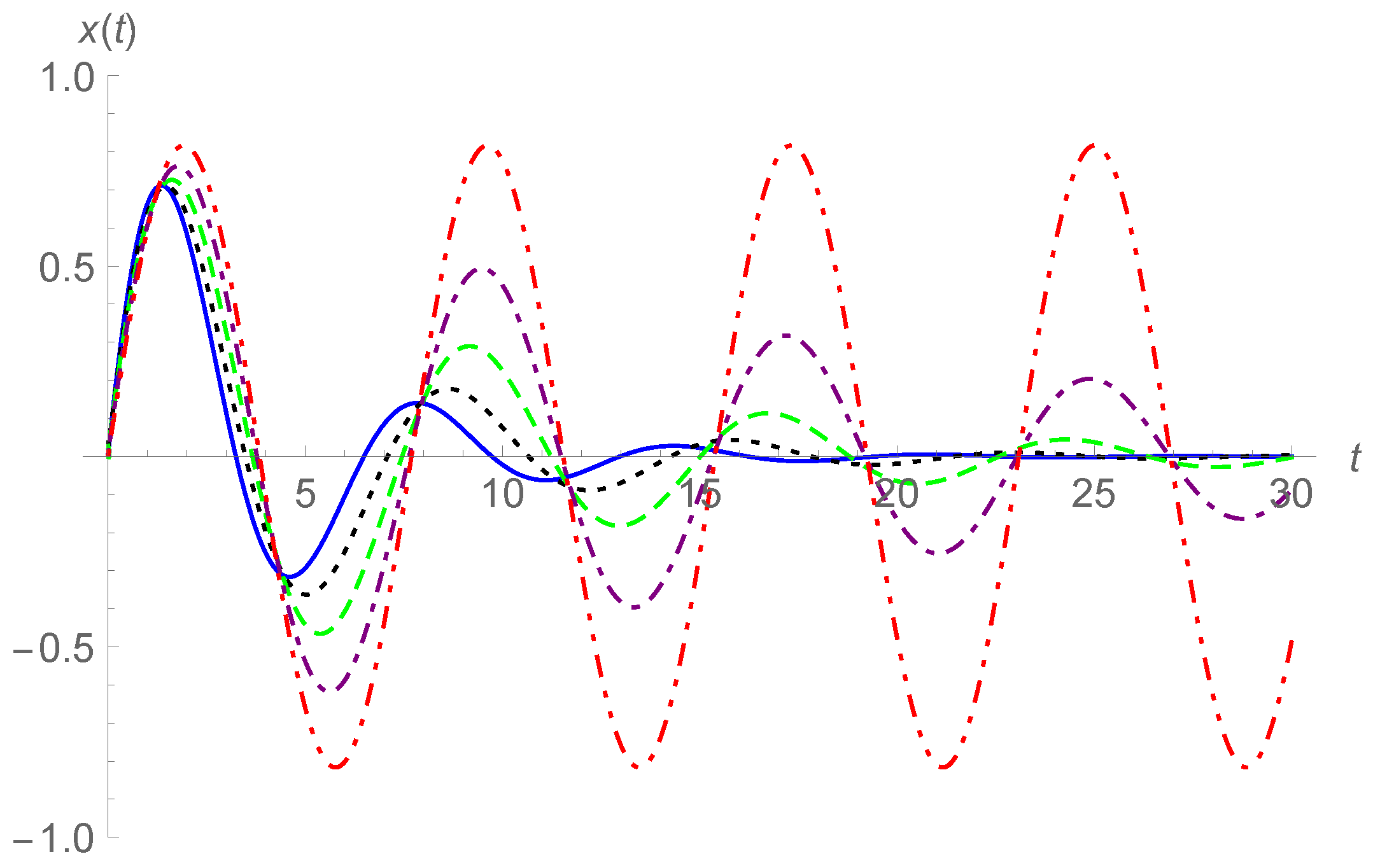
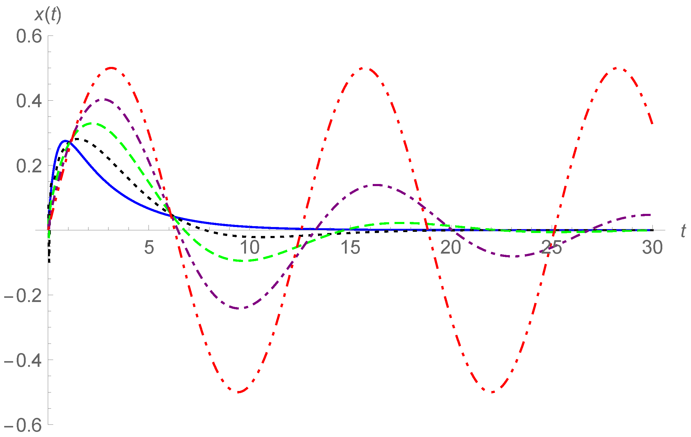
By taking $m=k=1$ and the sum of $n=0$ through $n=80$ in Equation (17), the curves of $x(t)$ are plotted in Figure 1 and Figure 2 for $c=0.5$ and different values of $\alpha$, and in Figure 3 for $c=3$ and $\alpha =0,0.25,0.5,0.75$, and 1. In Figure 1 and Figure 2, the ranges of t are limited in $0\le t\le 15$, and in Figure 3, the range is $0\le t\le 9$. For extended ranges of t, divergent curves may be observed. In addition, we did not plot curves of $c=3$ and $1<\alpha <2$ since in this case, convergence of the series slows down, especially for the case of $\alpha$ approaching 2.

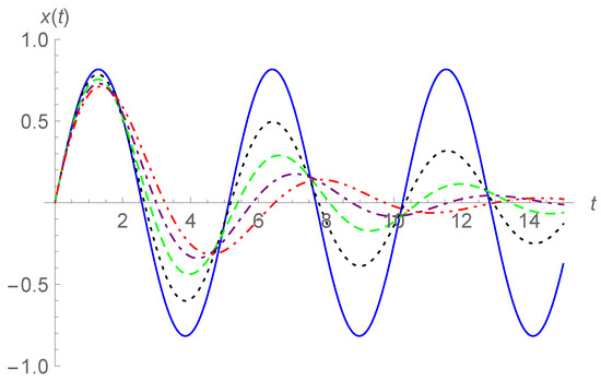
Figure 1. Curves of $x(t)$ for $m=k=1,c=0.5$ and for $\alpha =$0 (solid line), 0.25 (dotted line), 0.5 (dashed line), 0.75 (dotted-dashed line), and 1 (dotted-dotted-dashed line).

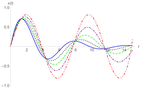
Figure 2. Curves of $x(t)$ for $m=k=1,c=0.5$ and for $\alpha =$1 (solid line), 1.25 (dotted line), 1.5 (dashed line), 1.75 (dotted-dashed line), and 2 (dotted-dotted-dashed line).

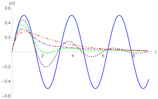
Figure 3. Curves of $x(t)$ for $m=k=1,c=3$ and for $\alpha =$0 (solid line), 0.25 (dotted line), 0.5 (dashed line), 0.75 (dotted-dashed line), and 1 (dotted-dotted-dashed line).

We notice that the formula for the Mittag–Leffler function

$$\frac{d^j}{d{z}^j}\left(z^j{E}_{\alpha ,\beta }(z)\right)=\sum _{l=0}^{+\infty }\frac{(j+l)!}{l!}\frac{z^l}{\mathsf{\Gamma }(\alpha l+\beta )},$$

(19)

where the two-parameter Mittag–Leffler function is defined as

$$E_{\alpha ,\beta }(z)=\sum _{l=0}^{+\infty }\frac{z^l}{\mathsf{\Gamma }(\alpha l+\beta )},\alpha >0,\beta >0.$$

(20)

Thus, the response (16) may be expressed as

$$x(t)=\sum _{j=0}^{+\infty }\frac{{(-k)}^j{t}^{2j+1}}{j!m^{j+1}}{g}_j\left(-\frac{c{t}^{2-\alpha }}{m}\right),\mathrm{where}{g}_j(z)=\frac{d^j}{d{z}^j}\left(z^j{E}_{2-\alpha ,2j+2}(z)\right).$$

(21)

The Integer-Order Cases

When $\alpha =1$, the response in Equation (17) can be expressed by using the Kummer hypergeometric function

$$\begin{array}{ccc}\hfill x(t;\alpha =1)& =& \sum _{n=0}^{+\infty }\frac{t}{(n+1)!m}{\left(-\frac{ct}{m}\right)}^n{}_1{F}_1\left(-n;2+n;\frac{-kt}{c}\right).\hfill \end{array}$$

(22)

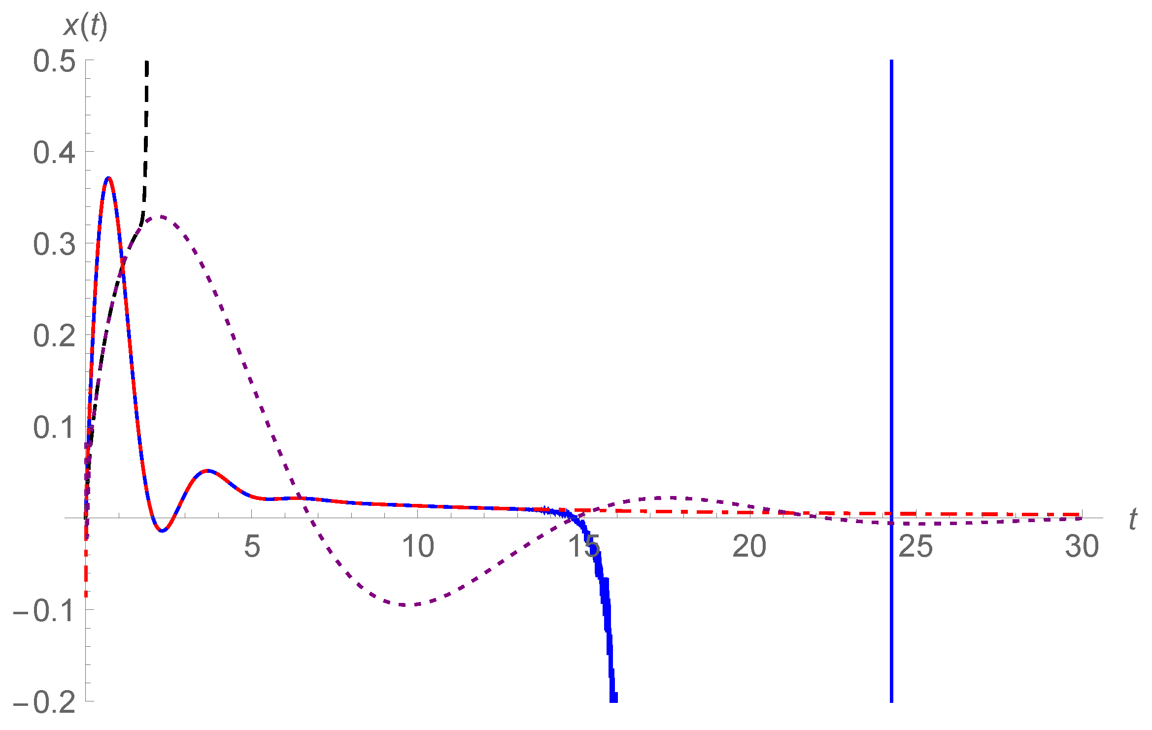
Here, we obtain the united series expressions for the three subcases, overdamping, criticaldamping, and underdamping, by exploiting the Kummer hypergeometric function. In Figure 4, the sum of the first 81 terms in Equation (22) is used to generate the curves of $x(t;\alpha =1)$, where c = 3, 2, and 1 correspond to overdamping, criticaldamping, and underdamping, respectively.

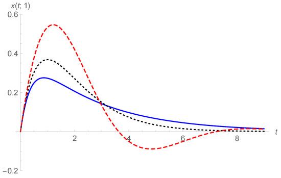
Figure 4. Curves of $x(t;\alpha =1)$ for $m=k=1$ and $c=3$ (solid line), $c=2$ (dotted line), and $c=1$ (dashed line).

For the case $\alpha =0$, upon using the binomial theorem, Equation (17) becomes

$$\begin{array}{ccc}\hfill x(t)& =& \sum _{n=0}^{+\infty }\sum _{j=0}^n\frac{n!}{j!(n-j)!}{\left(\frac{k}{c}\right)}^j\frac{{(-c)}^n{t}^{2n+1}}{m^{n+1}(2n+1)!}\hfill \\ & =& \sum _{n=0}^{+\infty }\frac{{(-1)}^n{(k+c)}^n{t}^{2n+1}}{m^{n+1}(2n+1)!}\hfill \\ & =& \frac{1}{\sqrt{m(k+c)}}sin\left(\sqrt{\frac{k+c}{m}}t\right),\hfill \end{array}$$

(23)

which is consistent with Equation (7).

For the case $\alpha =2$, Equation (16) is convergent under the condition $c<m$, and upon using the series expansion (13), it is reduced to the periodic oscillation as in Equation (8):

$$\begin{array}{ccc}\hfill x(t)& =& \sum _{j=0}^{+\infty }\frac{{(-k)}^j}{j!}\sum _{l=0}^{\infty }\frac{(l+j)!}{l!}{\left(-\frac{c}{m}\right)}^l\frac{t^{2j+1}}{m^{j+1}(2j+1)!}\hfill \\ & =& \sum _{j=0}^{+\infty }{(-1)}^j\frac{k^j{t}^{2j+1}}{{(m+c)}^{j+1}(2j+1)!}\hfill \\ & =& \frac{1}{\sqrt{(m+c)k}}sin\left(\sqrt{\frac{k}{m+c}}t\right).\hfill \end{array}$$

(24)

3. Solution Rapidly Convergent for Large t

We pursue the inverse Laplace transform of Equation (5) by using the complex inversion integral formula, alias Bromwich’s integral formula,

$$x(t)=\frac{1}{2\pi \mathrm{i}}{\int }_{\mathrm{Br}}X(s)e^{st}ds=\frac{1}{2\pi \mathrm{i}}{\int }_{\mathrm{Br}}\frac{1}{m{s}^2+c{s}^{\alpha }+k}{e}^{st}ds.$$

(25)

In the above formula, Br denotes the Bromwich path, namely the straight line from $s=\sigma -\mathrm{i}\infty$ to $s=\sigma +\mathrm{i}\infty$, where $\sigma$ is chosen so that all the singularities of the integrand lie to the left of the line.

For the non-integer case, the original point $s=0$ is a branch point of the integrand. We make a branch cut along the negative real axis and consider the problem on the principal Riemann surface. In addition, for the non-integer case, the Laplace transform $X(s)$ always has a pair of conjugated simple poles with a negative real part, i.e., the characteristic equation $m{s}^2+c{s}^{\alpha }+k=0$ has a pair of conjugated complex roots only if $m,c,k>0$ [18,19]. We denote the conjugated complex roots by $s_{1,2}=a\pm b\mathrm{i}$, where $a<0$ and $b>0$.

Due to the residue theorem and Jordan’s lemma, we can rewrite the right hand side of Equation (25) as the sum of residues plus a Hankel contour integral, i.e.,

$$x(t)=x_1(t)+x_2(t),$$

(26)

where

$$x_1(t)=\sum _{j=1}^2\mathrm{Res}\left[\frac{e^{st}}{m{s}^2+c{s}^{\alpha }+k},s_j\right],x_2(t)=\frac{1}{2\pi \mathrm{i}}{\int }_{\mathrm{Ha}}\frac{e^{st}}{m{s}^2+c{s}^{\alpha }+k}ds,$$

(27)

where Ha denotes the Hankel path, a loop which starts from $-\infty$ along the lower side of the negative real axis, encircles the origin counterclockwise, and ends at $-\infty$ along the upper side of the negative real axis.

Calculating the residues in Equation (27), we obtain

$$\begin{array}{ccc}\hfill x_1(t)& =& \frac{e^{s_{1}t}}{2m{s}_1+\alpha c{s}_1^{\alpha -1}}+\frac{e^{s_{2}t}}{2m{s}_2+\alpha c{s}_2^{\alpha -1}}.\hfill \end{array}$$

Considering the relation $s_1=\overline{s_2}$, we have

$$\begin{array}{ccc}\hfill x_1(t)& =& 2\mathrm{Re}\left(\frac{e^{s_{1}t}}{2m{s}_1+\alpha c{s}_1^{\alpha -1}}\right),\hfill \end{array}$$

(28)

where $\mathrm{Re}(·)$ denotes the real part. Utilizing the relation $m{s}_1^2+c{s}_1^{\alpha }+k=0,$ we rewrite Equation (28) as

$$\begin{array}{c}\hfill x_1(t)=2\mathrm{Re}\left(\frac{s_1{e}^{s_{1}t}}{2m{s}_1^2+\alpha c{s}_1^{\alpha }}\right)=2\mathrm{Re}\left(\frac{s_1{e}^{s_{1}t}}{2m{s}_1^2-\alpha k-\alpha m{s}_1^2}\right).\end{array}$$

(29)

Substituting $s_1=a+b\mathrm{i}$, using the equality $e^{\mathrm{i}bt}=cos(bt)+\mathrm{i}sin(bt)$, and then extracting the real part, we obtain

$$x_1(t)=e^{at}(Asin(bt)+Bcos(bt)),$$

(30)

where

$$\begin{array}{ccc}\hfill A& =& \frac{2bm(2-\alpha )(a^2+b^2)+2\alpha bk}{{(m(2-\alpha )(a^2-b^2)-\alpha k)}^2+4a^2{b}^2{m}^2{(2-\alpha )}^2},\hfill \end{array}$$

(31)

$$\begin{array}{ccc}\hfill B& =& \frac{2am(2-\alpha )(a^2+b^2)-2\alpha ak}{{(m(2-\alpha )(a^2-b^2)-\alpha k)}^2+4a^2{b}^2{m}^2{(2-\alpha )}^2}.\hfill \end{array}$$

(32)

Obviously, in the fractional case, $x_1(t)$ represents a harmonic damped oscillation. We note that for the case of $\alpha =1$ and $c^2-4mk\ge 0$, $x_1(t)$ must be replaced by the expressions in (6).

For $x_2(t)$, the Hankel path integral may be divided into three parts:

$$\begin{array}{ccc}\hfill x_2(t)& =& \frac{1}{2\pi \mathrm{i}}\left({\int }_{s=r{e}^{\mathrm{i}\pi }(0:\infty )}\frac{e^{st}}{m{s}^2+c{s}^{\alpha }+k}ds+{\int }_{s=r{e}^{-\mathrm{i}\pi }(\infty :0)}\frac{e^{st}}{m{s}^2+c{s}^{\alpha }+k}\right.\hfill \\ & & \left.+\underset{\epsilon \to 0^{+}}{lim}{\int }_{C(\epsilon )}\frac{e^{st}}{m{s}^2+c{s}^{\alpha }+k}ds\right),\hfill \end{array}$$

(33)

where the integral paths are explained as follows: in the first integral, the path is from $s=0$ to ∞ along the upper side of the negative real axis; in the second integral, the path is from $s=\infty$ to 0 along the lower side of the negative real axis; and in the third integral, the path is the small circle counterclockwise:

$$C(\epsilon ):s=\epsilon e^{\mathrm{i}\theta },\epsilon >0,-\pi <\theta <\pi .$$

(34)

It is easy to prove that

$$\begin{array}{c}\hfill \underset{\epsilon \to 0^{+}}{lim}{\int }_{C(\epsilon )}\frac{e^{st}}{m{s}^2+c{s}^{\alpha }+k}ds=\underset{\epsilon \to 0^{+}}{lim}{\int }_{-\pi }^{\pi }\frac{e^{\epsilon t{e}^{\mathrm{i}\theta }}}{m{\epsilon }^2{e}^{\mathrm{i}2\theta }+c{\epsilon }^{\alpha }{e}^{\mathrm{i}\alpha \theta }+k}\epsilon e^{\mathrm{i}\theta }\mathrm{i}d\theta =0.\end{array}$$

(35)

Consequently, we obtain

$$\begin{array}{ccc}\hfill x_2(t)& =& \frac{-1}{2\pi \mathrm{i}}{\int }_0^{+\infty }\left(\frac{e^{-rt}}{m{r}^2+c{r}^{\alpha }{e}^{\mathrm{i}\pi \alpha }+k}-\frac{e^{-rt}}{m{r}^2+c{r}^{\alpha }{e}^{-\mathrm{i}\pi \alpha }+k}\right)dr.\hfill \end{array}$$

Considering the two terms in brackets are conjugated we have

$$\begin{array}{ccc}\hfill x_2(t)& =& \frac{-1}{\pi }{\int }_0^{+\infty }\mathrm{Im}\left(\frac{e^{-rt}}{m{r}^2+c{r}^{\alpha }{e}^{\mathrm{i}\pi \alpha }+k}\right)dr,\hfill \end{array}$$

(36)

where $\mathrm{Im}(·)$ denotes the imaginary part. Calculating the imaginary part leads to

$$\begin{array}{c}\hfill x_2(t)=x_2(t;\alpha )=\frac{csin(\pi \alpha )}{\pi }{\int }_0^{+\infty }q(r,\alpha )e^{-rt}dr,\end{array}$$

(37)

where

$$\begin{array}{c}\hfill q(r,\alpha )=\frac{r^{\alpha }}{{(m{r}^2+k+c{r}^{\alpha }cos(\pi \alpha ))}^2+{(c{r}^{\alpha }sin(\pi \alpha ))}^2}.\end{array}$$

(38)

The infinite integral in Equation (37) converges rapidly for a large t due to the negative exponential function $e^{-rt}$ in the integrand. It is easy to conclude from Equations (37) and (38) that when $0<\alpha <1$, $x_2(t)$ is positive and decreases monotonically and approaches to zero as $t\to +\infty$, and when $\alpha >1$, $x_2(t)$ is negative and increases monotonically and approaches to zero as $t\to +\infty$. When $0<\alpha <1$, $x_2(t)$ is completely monotone, i.e., ${(-1)}^n{x}_2^{(n)}(t)\ge 0$ for all $n=0,1,2,\dots$. When $1<\alpha <2$, $-x_2(t)$ is completely monotone.

We notice that the infinite integral in Equation (37) is in the Laplace pattern, and $q(r)$ has the asymptotic expression

$$q(r,\alpha )\sim \frac{1}{k^2}{r}^{\alpha },r\to 0.$$

(39)

Thus, the asymptotic behaviour of $x_2(t)$ is obtained upon using the Watson lemma

$$x_2(t)\sim \frac{csin(\pi \alpha )}{\pi k^2}\frac{\mathsf{\Gamma }(\alpha +1)}{t^{\alpha +1}},t\to +\infty .$$

(40)

Hence, the response $x(t)=x_1(t)+x_2(t)$ is a superposition of a damped oscillation dying out in a negative exponent rate and a monotonic restoration decaying in a negative power rate,

$$x(t)=x_1(t)+\frac{csin(\pi \alpha )}{\pi }{\int }_0^{+\infty }q\left(r,\alpha \right)e^{-rt}dr.$$

(41)

The derivatives of $x(t)$ have almost the same formations. Therefore, considering that the negative exponent function is an infinitesimal of higher order than the negative power function as $t\to +\infty$, it is deduced that the response $x(t)=x_1(t)+x_2(t)$ has the same asymptotic behaviour as $x_2(t)$, and $x(t)$ evolves from initially probably oscillating to decreasing monotonically and approaching zero for the case $0<\alpha <1$, while increasing monotonically and approaching zero for the case $1<\alpha <2$.

Although the infinite integral in Equation (37) can be directly computed by using MATLAB or MATHEMATICA, we prefer to introduce a sort of quadrature formula. In Equation (37), the infinite integral in the Laplace pattern is appropriate for numerical calculation by using the Gauss–Laguerre quadrature formula. In fact, introducing the new integration variable $u=rt$, Equation (37) can be rewritten in the form

$$\begin{array}{c}\hfill x_2(t)=\frac{csin(\pi \alpha )}{\pi t}{\int }_0^{+\infty }q\left(\frac{u}{t},\alpha \right)e^{-u}du.\end{array}$$

(42)

Thus, applying the Gauss–Laguerre quadrature formula, we have

$$\begin{array}{c}\hfill x_2(t)\doteq \frac{csin(\pi \alpha )}{\pi t}\sum _{j=1}^n{w}_{j}q\left(\frac{u_j}{t},\alpha \right),\end{array}$$

(43)

where $u_j$ is the j-th zero of the Laguerre polynomial $L_n(u)$, and the weight $w_j$ is given by

$$w_j=\frac{{(n!)}^2}{u_j{[L_n^{{}^{\prime }}(u_j)]}^2},j=1,2,\dots ,n.$$

(44)

Finally, the solution $x(t)$ can be calculated as the approximate analytical expression

$$\begin{array}{c}\hfill x(t)\doteq x_1(t)+\frac{csin(\pi \alpha )}{\pi t}\sum _{j=1}^n{w}_{j}q\left(\frac{u_j}{t},\alpha \right).\end{array}$$

(45)

The Integer-Order Cases

For the integer-order case $\alpha =1$, 2, or 3; $x_2(t)=0$; and there is only the contribution from residues, $x_1(t)$, for the solution $x(t)$. Now, we specialize $x_1(t)$ in Equation (30). If $\alpha =1$, we have $a=-\frac{c}{2m},b=\frac{\sqrt{4mk-c^2}}{2m}.$ Substituting them into Equations (31) and (32), we find that $A=\frac{2}{\sqrt{4mk-c^2}}$ and $B=0$. Thus, from Equation (30), we obtain the underdamping result of the case $\alpha =1$ as in Equation (6). If $\alpha =0,$ then $a=0$ and $b=\sqrt{\frac{k+c}{m}}$. It follows from Equations (31) and (32) that $A=\frac{1}{mb}$ and $B=0$. From Equation (30), the response in Equation (7) is revealed. If $\alpha =2$, then $a=0$ and $b=\sqrt{\frac{k}{m+c}}$. It follows from Equations (31) and (32) that $A=b/k$ and $B=0$. From Equation (30), the response degenerates to that in Equation (8).

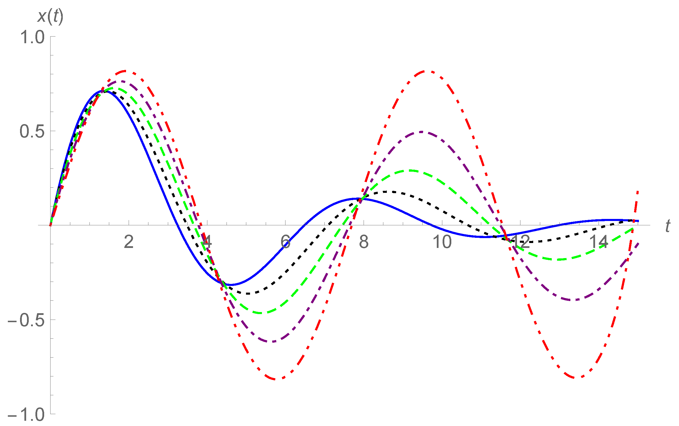
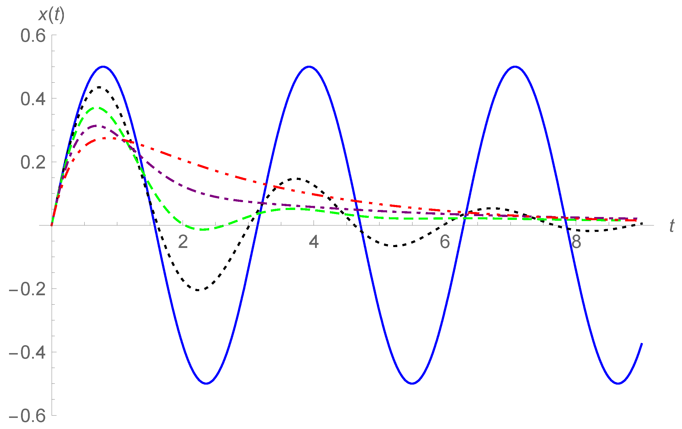
By taking $m=k=1$ and $n=50$ in Equation (45), the curves of $x(t)$ are plotted in Figure 5 and Figure 6 for $c=0.5$ and in Figure 7 and Figure 8 for $c=3$. Here, larger ranges of t are shown than in Figure 1, Figure 2 and Figure 3. In Figure 5 and Figure 6, the responses are the underdamping case for $\alpha =1$, while in Figure 7 and Figure 8, the responses are the overdamping case for $\alpha =1$. Finally, in order to compare intuitionally the two analytical forms in Equations (17) and (45), we plot their corresponding response curves together. We take $m=k=1$, $\alpha =0.5$ and 1.5, and the curves of $x(t)$ are plotted in Figure 9 for $c=0.5$, while in Figure 10 for $c=3$. The series in Equation (17) is approximated by the sum of the first 81 terms, while in Equation (45), we take $n=50$. The analytical form in Equation (45) gives effective results on the whole displayed interval $0<t<30$ in Figure 9 and Figure 10 by red dotted-dashed lines and purple dotted lines, while the analytical form in Equation (17) outputs effective curves for $t<25$ in Figure 9, and for even smaller intervals in Figure 10.

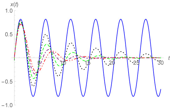
Figure 5. Curves of $x(t)$ for $m=k=1,c=0.5$, and for $\alpha =$0 (solid line), 0.25 (dotted line), 0.5 (dashed line), 0.75 (dotted-dashed line), and 1 (dotted-dotted-dashed line).

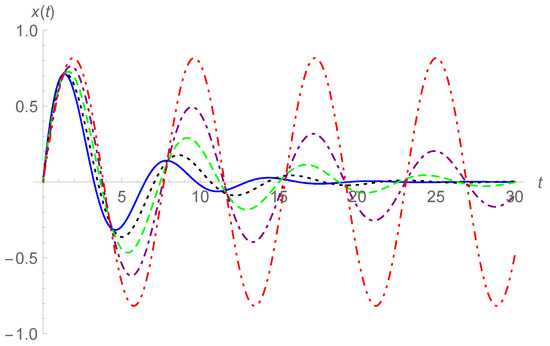
Figure 6. Curves of $x(t)$ for $m=k=1,c=0.5$, and for $\alpha =$1 (solid line), 1.25 (dotted line), 1.5 (dashed line), 1.75 (dotted-dashed line), and 2 (dotted-dotted-dashed line).

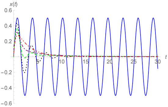
Figure 7. Curves of $x(t)$ for $m=k=1,c=3$, and for $\alpha =$0 (solid line), 0.25 (dotted line), 0.5 (dashed line), 0.75 (dotted-dashed line), and 1 (dotted-dotted-dashed line).

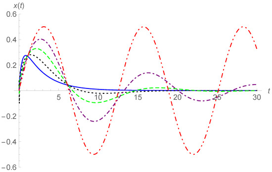
Figure 8. Curves of $x(t)$ for $m=k=1,c=3$, and for $\alpha =$1 (solid line), $\alpha =$1.25 (dotted line), 1.5 (dashed line), 1.75 (dotted-dashed line), and 2 (dotted-dotted-dashed line).

Figure 9. Curves of $x(t)$ for $m=k=1,c=0.5$ and for $\alpha =0.5$ (solid and dotted-dashed lines) and 1.5 (dashed and dotted lines), where solid and dashed lines are from Equation (17), dotted-dashed and dotted lines from Equation (45).

Figure 10. Curves of $x(t)$ for $m=k=1,c=3$, and for $\alpha =0.5$ (solid and dotted-dashed lines) and 1.5 (dashed and dotted lines), where solid and dashed lines are from Equation (17), and dotted-dashed and dotted lines from Equation (45).

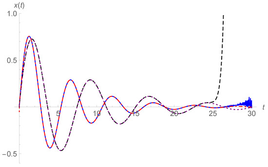
4. Conclusions

We have investigated the impulse response of the fractional oscillation equation, where the damping term is characterized by means of the Riemann–Liouville fractional derivative with the order $\alpha$ satisfying $0\le \alpha \le 2$. Two different forms of the response are obtained by using the two different methods of inverse Laplace transform, i.e., (i) expanding into a series of a negative power of s in the Laplace domain and then inverting the series term by term and (ii) using the complex inversion integral formula, residue theorem, Jordan’s lemma, and Gauss–Laguerre quadrature formula. Method (i) leads to a series solution composed of positive powers of t, which converges rapidly for a small t, while method (ii) derives a sum of a damped harmonic oscillation with negative exponential amplitude and a decayed function in the form of an infinite integral, where the infinite integral converges rapidly for a large t. Furthermore, due to the infinite integral in the Laplace pattern, the Gauss–Laguerre quadrature formula is appropriate for a numerical calculation to generate an analytical approximation to the response. The asymptotic behaviours for a small t and large t are also obtained from the two forms of response. The results include that of the integer-order cases, $\alpha =$ 0, 1, and 2.

References

- Miller, K.S.; Ross, B. An Introduction to the Fractional Calculus and Fractional Differential Equations; Wiley: New York, NY, USA, 1993. [Google Scholar]
- Kiryakova, V. Generalized Fractional Calculus and Applications (Pitman Res. Notes in Math. Ser., Vol. 301); Longman Scientific & Technical and John Wiley & Sons, Inc.: Harlow, UK; New York, NY, USA, 1994. [Google Scholar]
- Mainardi, F. Fractional Calculus and Waves in Linear Viscoelasticity; Imperial College: London, UK, 2010. [Google Scholar]
- Podlubny, I. Fractional Differential Equations; Academic: San Diego, CA, USA, 1999. [Google Scholar]
- Klafter, J.; Lim, S.C.; Metzler, R. (Eds.) Fractional Dynamics: Recent Advances; World Scientific: Singapore, 2011. [Google Scholar]
- Kilbas, A.A.; Srivastava, H.M.; Trujillo, J.J. Theory and Applications of Fractional Differential Equations; Elsevier: Amsterdam, The Netherlands, 2006. [Google Scholar]
- West, B.J. Fractional Calculus View of Complexity—Tomorrow’s Science; CRC Press/Taylor & Francis Group: Boca Raton, CO, USA; London, UK; New York, NY, USA, 2016. [Google Scholar]
- Monje, C.A.; Chen, Y.Q.; Vinagre, B.M.; Xue, D.; Feliu, V. Fractional-Order Systems and Controls, Fundamentals and Applications; Springer: London, UK, 2010. [Google Scholar]
- Li, M. Theory of Fractional Engineering Vibrations; De Gruyter: Berlin, Germany; Boston, MA, USA, 2021. [Google Scholar]
- Scott-Blair, G.W. Survey of General and Applied Rheology; Pitman: London, UK, 1949. [Google Scholar]
- Bagley, R.L.; Torvik, P.J. A generalized derivative model for an elastomer damper. Shock Vib. Bull. 1979, 49, 135–143. [Google Scholar]
- Koeller, R.C. Applications of fractional calculus to the theory of viscoelasticity. J. Appl. Mech. 1984, 51, 299–307. [Google Scholar] [CrossRef]
- Duan, J.S.; Hu, D.C.; Chen, Y.Q. Simultaneous characterization of relaxation, creep, dissipation, and hysteresis by fractional-order constitutive models. Fractal Fract. 2021, 5, 36. [Google Scholar] [CrossRef]
- Bagley, R.L.; Torvik, P.J. On the appearance of the fractional derivative in the behavior of real materials. J. Appl. Mech. 1984, 51, 294–298. [Google Scholar]
- Beyer, H.; Kempfle, S. Definition of physically consistent damping laws with fractional derivatives. ZAMM-J. Appl. Math. Mech. 1995, 75, 623–635. [Google Scholar] [CrossRef]
- Achar, B.N.N.; Hanneken, J.W.; Clarke, T. Response characteristics of a fractional oscillator. Physica A 2002, 309, 275–288. [Google Scholar] [CrossRef]
- Rossikhin, Y.A.; Shitikova, M.V. Applications of fractional calculus to dynamic problems of linear and nonlinear hereditary mechanisms of solids. Appl. Mech. Rev. 1997, 50, 15–67. [Google Scholar] [CrossRef]
- Naber, M. Linear fractionally damped oscillator. Int. J. Differ. Equ. 2010, 2010, 197020. [Google Scholar] [CrossRef] [PubMed] [Green Version]
- Liu, L.L.; Duan, J.S. A detailed analysis for the fundamental solution of fractional vibration equation. Open Math. 2015, 13, 826–838. [Google Scholar] [CrossRef] [Green Version]
- Li, M. Three classes of fractional oscillators. Symmetry 2018, 10, 40. [Google Scholar] [CrossRef] [Green Version]
- Wang, Z.H.; Hu, H.Y. Stability of a linear oscillator with damping force of the fractional-order derivative. Sci. China Ser. G 2010, 53, 345–352. [Google Scholar] [CrossRef]
- Li, Y.; Duan, J.S. The periodic response of a fractional oscillator with a spring-pot and an inerter-pot. J. Mech. 2021, 37, 108–117. [Google Scholar] [CrossRef]
- Zhang, W.; Liao, S.K.; Shimizu, N. Dynamic behaviors of nonlinear fractional-order differential oscillator. J. Mech. Sci. Tech. 2009, 23, 1058–1064. [Google Scholar] [CrossRef]
- Shen, Y.; Yang, S.; Xing, H.; Gao, G. Primary resonance of Duffing oscillator with fractional-order derivative. Commun. Nonlinear Sci. Numer. Simul. 2012, 17, 3092–3100. [Google Scholar] [CrossRef]
- Li, M. Theory of vibrators with variable-order fractional forces. arXiv 2021, arXiv:2107.02340. [Google Scholar]
Publisher’s Note: MDPI stays neutral with regard to jurisdictional claims in published maps and institutional affiliations. |
© 2021 by the authors. Licensee MDPI, Basel, Switzerland. This article is an open access article distributed under the terms and conditions of the Creative Commons Attribution (CC BY) license (https://creativecommons.org/licenses/by/4.0/).