Monotone Iterative and Upper–Lower Solution Techniques for Solving the Nonlinear ψ−Caputo Fractional Boundary Value Problem

Abstract

The objective of this paper is to study the existence of extremal solutions for nonlinear boundary value problems of fractional differential equations involving the $\mathsf{\psi }-$Caputo derivative ${}^C{\mathbb{D}}_{a^{+}}^{\sigma ;\mathsf{\psi }}\varrho \left(\mathrm{t}\right)=\mathcal{V}(\mathrm{t},\varrho \left(\mathrm{t}\right))$ under integral boundary conditions $\varrho \left(a\right)=\lambda {\mathbb{I}}^{\nu ;\mathsf{\psi }}\varrho \left(\eta \right)+\delta$. Our main results are obtained by applying the monotone iterative technique combined with the method of upper and lower solutions. Further, we consider three cases for ${\mathsf{\psi }}^{*}\left(\mathrm{t}\right)$ as $\mathrm{t}$, Caputo, $2^{\mathrm{t}}$, $\sqrt{\mathrm{t}}$, and Katugampola (for $\rho =0.5)$ derivatives and examine the validity of the acquired outcomes with the help of two different particular examples.

1. Introduction

The notion of fractional calculus refers to the last three centuries and it can be described as the generalization of classical calculus to orders of integration and differentiation that are not necessarily integers. Many researchers have used fractional calculus in different scientific areas [1,2,3,4].

In the literature, various definitions of the fractional-order derivative have been suggested. The oldest and the most famous ones advocate for the use of the Riemann–Liouville and Caputo settings. One of the most recent definitions of a fractional derivative was delivered by Kilbas et al., where the fractional differentiation of a function with respect to another function in the sense of Riemann–Liouville was introduced [5]. They further defined appropriate weighted spaces and studied some of their properties by using the corresponding fractional integral. In [6], Almaida defined the following new fractional derivative and integrals of a function with respect to some other function:

$$\begin{array}{cc}\hfill {\mathbb{D}}_{a^{+}}^{\sigma ,{\mathsf{\psi }}^{*}}\varrho \left(\mathfrak{x}\right)& :={\left(\frac{1}{{{\mathsf{\psi }}^{*}}^{\prime }\left(\xi \right)}\frac{\mathrm{d}}{\mathrm{d}\mathfrak{x}}\right)}^n{\mathbb{I}}_{a^{+}}^{n-\sigma ,{\mathsf{\psi }}^{*}}\varrho \left(\mathfrak{x}\right)\hfill \\ \hfill & ={\left(\frac{1}{{{\mathsf{\psi }}^{*}}^{\prime }\left(\xi \right)}\frac{\mathrm{d}}{\mathrm{d}\mathfrak{x}}\right)}^n{\int }_a^{\mathfrak{x}}\frac{{{\mathsf{\psi }}^{*}}^{\prime }\left(\xi \right)}{\Gamma (n-\sigma )}{\left({\mathsf{\psi }}^{*}\left(\mathfrak{x}\right)-{\mathsf{\psi }}^{*}\left(\xi \right)\right)}^{n-\sigma -1}\varrho \left(\xi \right)\mathrm{d}\xi ,\hfill \end{array}$$

(1)

where $n=\left[\sigma \right]+1$ and 

$${\mathbb{I}}_{a^{+}}^{\sigma ,{\mathsf{\psi }}^{*}}\varrho \left(\mathfrak{x}\right):={\int }_a^{\mathfrak{x}}\frac{{\mathsf{\psi }}^{\prime }\left(\xi \right)}{\Gamma \left(\sigma \right)}{\left({\mathsf{\psi }}^{*}\left(\mathfrak{x}\right)-{\mathsf{\psi }}^{*}\left(\xi \right)\right)}^{\sigma -1}\varrho \left(\xi \right)\mathrm{d}\xi ,$$

(2)

respectively. He called the fractional derivative the $\mathsf{\psi }-$Caputo fractional operator. In the above definitions, we get the Riemann–Liouville and Hadamard fractional operators whenever we consider ${\mathsf{\psi }}^{*}\left(\mathfrak{x}\right)=\mathfrak{x}$ or ${\mathsf{\psi }}^{*}\left(\mathfrak{x}\right)=ln\mathfrak{x}$, respectively. Many researchers used this $\mathsf{\psi }-$Caputo fractional derivative (see [7,8,9,10,11,12,13] and the references therein). Abdo et al., in [14], investigated the BVP for a fractional differential equation (FDE) involving ${\mathsf{\psi }}^{*}$ operator and was given as

$${\mathbb{D}}_{{\mathrm{t}}_1^{+}}^{n-\sigma ,{\mathsf{\psi }}^{*}}\varrho \left(\mathrm{t}\right)=\mathcal{V}(\mathrm{t},\varrho \left(\mathrm{t}\right)),\mathrm{t}\in ı=:[{\mathrm{t}}_1,{\mathrm{t}}_2],$$

${\varrho }_{{\mathsf{\psi }}^{*}}^{\left[k\right]}\left({\mathrm{t}}_1\right)={\varrho }_{{\mathrm{t}}_1}^k,(k=0,1,2,\cdots ,n-2)$, ${\varrho }_{{\mathsf{\psi }}^{*}}^{[n-1]}\left({\mathrm{t}}_2\right)={\varrho }_{{\mathrm{t}}_2}$. For more details on the development of the theory of fractional differential equations, one can refer to [15,16,17,18,19,20]. In order to establish existence theory, researchers have used diverse techniques of nonlinear analysis consisting of fixed-point theory, hybrid fixed-point theory, topological degree theory, and measure of noncompactness [21,22,23,24]. However, the use of the monotone iterative technique ($\mathbb{MIT}$) along with the method of upper and lower solutions (u-l solutions) for solving a BVP involving the operator remains rare.

In the present paper, we are interested in the $\mathbb{MIT}$ blended with the method of upper and lower solutions to prove the existence of extremal solutions for the following BVP of an FDE involving the operator

$$\left\{\begin{array}{c}{}^C{\mathbb{D}}_{{\mathrm{t}}_1^{+}}^{\sigma ;{\mathsf{\psi }}^{*}}\varrho \left(\mathrm{t}\right)=\mathcal{V}(\mathrm{t},\varrho \left(\mathrm{t}\right)),\mathrm{t}\in ı,\hfill \\ \varrho \left({\mathrm{t}}_1\right)=\lambda {\mathbb{I}}^{\nu ;{\mathsf{\psi }}^{*}}\varrho \left(\eta \right)+\delta ,\hfill \end{array}\right.$$

(3)

where ${}^C{\mathbb{D}}^{\sigma ;{\mathsf{\psi }}^{*}}$ is the operator (1) of order $0<\sigma ,\nu \le 1$, ${\mathbb{I}}^{\sigma ;{\mathsf{\psi }}^{*}}$ is the operator (2), the function $\mathcal{V}:[{\mathrm{t}}_1,{\mathrm{t}}_2]\times \mathbb{R}\to \mathbb{R}$ is continuous, $\lambda$ and $\delta$ are real constants, and $\eta \in ({\mathrm{t}}_1,{\mathrm{t}}_2)$. It is worth mentioning that the $\mathbb{MIT}$ is efficiently used in the literature to investigate the existence of extremal solutions to many applied problems of nonlinear equations [25,26,27,28,29,30,31,32,33,34,35,36,37,38].

The rest of this paper is organized as follows. In Section 2, we recall some preliminary concepts, definitions, and lemmas that will act as prerequisites to proving the main results. The main results are stated and proved in Section 3. Finally, we give numerical examples to illustrate the correctness of the outcome.

2. Preliminaries

Let $\sigma >0$. The left-sided $\mathsf{\psi }-$Riemann–Liouville fractional integral (l-s-$\mathsf{\psi }$-RLfi) of order $\sigma$ for an integrable function $\varrho :ı\to \mathbb{R}$ with respect to another function ${\mathsf{\psi }}^{*}:ı\to \mathbb{R}$, which is an increasing differentiable function such that ${{\mathsf{\psi }}^{*}}^{\prime }\left(\mathrm{t}\right)\ne 0,(\forall \mathrm{t}\in ı)$, is defined as follows:

$${\mathbb{I}}_{{\mathrm{t}}_1^{+}}^{\sigma ;{\mathsf{\psi }}^{*}}\varrho \left(\mathrm{t}\right)=\frac{1}{\Gamma \left(\sigma \right)}{\int }_{{\mathrm{t}}_1}^{\mathrm{t}}{{\mathsf{\psi }}^{*}}^{\prime }\left(\xi \right){\left({\mathsf{\psi }}^{*}\left({\mathrm{t}}_1\right)-{\mathsf{\psi }}^{*}\left(\xi \right)\right)}^{\sigma -1}\varrho \left(\xi \right)\mathrm{d}\xi ,$$

(4)

where $\Gamma$ is the classical Euler Gamma function [5,6]. Appendix A Algorithm A1 shows the MATLAB lines for the calculation of the l-s-$\mathsf{\psi }$-RLfi. Let $n\in \mathbb{N}$ and ${\mathsf{\psi }}^{*}$, $\varrho \in C^n(ı,\mathbb{R})$ be two functions such that ${\mathsf{\psi }}^{*}$ is increasing and ${{\mathsf{\psi }}^{*}}^{\prime }\left(\mathrm{t}\right)\ne 0,(\forall \mathrm{t}\in ı)$. The left-sided $\mathsf{\psi }-$Riemann–Liouville fractional derivative (l-s-$\mathsf{\psi }$-RLfd) of a function $\varrho$ of order $\sigma$ is defined by

$$\begin{array}{cc}\hfill {\mathbb{D}}_{{\mathrm{t}}_1^{+}}^{\sigma ;{\mathsf{\psi }}^{*}}\varrho \left(\mathrm{t}\right)& ={\left(\frac{1}{{{\mathsf{\psi }}^{*}}^{\prime }\left(\mathrm{t}\right)}\frac{\mathrm{d}}{\mathrm{d}\mathrm{t}}\right)}^n{\mathbb{I}}_{{\mathrm{t}}_1^{+}}^{n-\sigma ;{\mathsf{\psi }}^{*}}\varrho \left(\mathrm{t}\right)\hfill \\ \hfill & =\frac{1}{\Gamma (n-\sigma )}{\left(\frac{1}{{{\mathsf{\psi }}^{*}}^{\prime }\left(\mathrm{t}\right)}\frac{\mathrm{d}}{\mathrm{d}\mathrm{t}}\right)}^n{\int }_{{\mathrm{t}}_1}^{\mathrm{t}}{{\mathsf{\psi }}^{*}}^{\prime }\left(\xi \right){({\mathsf{\psi }}^{*}\left(\mathrm{t}\right)-{\mathsf{\psi }}^{*}\left(\xi \right))}^{n-\sigma -1}\varrho \left(\xi \right)\mathrm{d}\xi ,\hfill \end{array}$$

(5)

where $n=\left[\sigma \right]+1$ [6]. Appendix A Algorithm A2 shows the MATLAB lines for the calculation of the l-s-$\mathsf{\psi }$-RLfd. In addition, the left-sided $\mathsf{\psi }-$Caputo fractional derivative (l-s-$\mathsf{\psi }$-Cfd) of a function $\varrho$ of order $\sigma$ is defined by

$$\begin{array}{cc}\hfill {}^C{\mathbb{D}}_{{\mathrm{t}}_1^{+}}^{\sigma ;{\mathsf{\psi }}^{*}}\varrho \left(\mathrm{t}\right)& ={\mathbb{I}}_{{\mathrm{t}}_1^{+}}^{n-\sigma ;{\mathsf{\psi }}^{*}}{\left(\frac{1}{{{\mathsf{\psi }}^{*}}^{\prime }\left(\mathrm{t}\right)}\frac{\mathrm{d}}{\mathrm{d}\mathrm{t}}\right)}^n\varrho \left(\mathrm{t}\right),\hfill \end{array}$$

where ${\mathsf{\psi }}^{*},\varrho \in C^n(ı,\mathbb{R})$ are two functions such that ${\mathsf{\psi }}^{*}$ is increasing, ${{\mathsf{\psi }}^{*}}^{\prime }\left(\mathrm{t}\right)\ne 0,(\forall \mathrm{t}\in ı)$, and $n=\left[\sigma \right]+1$ and $n=\sigma$ whenever $\sigma \notin \mathbb{N}$ and $\sigma \in \mathbb{N}$, respectively [6]. To simplify the notation, we use:

$${\varrho }_{{\mathsf{\psi }}^{*}}^{\left[n\right]}\left(\mathrm{t}\right)={\left(\frac{1}{{{\mathsf{\psi }}^{*}}^{\prime }\left(\mathrm{t}\right)}\frac{\mathrm{d}}{\mathrm{d}\mathrm{t}}\right)}^n\varrho \left(\mathrm{t}\right).$$

So,

$${}^C{\mathbb{D}}_{{\mathrm{t}}_1^{+}}^{\sigma ;{\mathsf{\psi }}^{*}}\varrho \left(\mathrm{t}\right)=\left\{\begin{array}{cc}{\displaystyle \frac{1}{\Gamma (n-\sigma )}{\int }_{\mathrm{t}}^{\mathrm{t}}{{\mathsf{\psi }}^{*}}^{\prime }\left(\xi \right){({\mathsf{\psi }}^{*}\left(\mathrm{t}\right)-{\mathsf{\psi }}^{*}\left(\xi \right))}^{n-\sigma -1}{\varrho }_{{\mathsf{\psi }}^{*}}^{\left[n\right]}\left(\xi \right)\mathrm{d}\xi ,}\hfill & \sigma \notin \mathbb{N},\hfill \\ {\varrho }_{{\mathsf{\psi }}^{*}}^{\left[n\right]}\left(\mathrm{t}\right),\hfill & \sigma \in \mathbb{N}.\hfill \end{array}\right.$$

(6)

Appendix A Algorithm A3 shows the MATLAB lines for the calculation of ${}^C{\mathbb{D}}_{{\mathrm{t}}_1^{+}}^{\sigma ;{\mathsf{\psi }}^{*}}\varrho \left(\mathrm{t}\right)$. If $\varrho \in C^n(ı,\mathbb{R})$, then the $\mathsf{\psi }$Cfd of order $\sigma$ of $\varrho$ is determined as ([6], Theorem 3):

$${}^C{\mathbb{D}}_{{\mathrm{t}}_1^{+}}^{\sigma ;{\mathsf{\psi }}^{*}}\varrho \left(t\right)={\mathbb{D}}_{{\mathrm{t}}_1^{+}}^{\sigma ;{\mathsf{\psi }}^{*}}\left[\varrho \left(\mathrm{t}\right)-\sum _{k=0}^{n-1}\frac{{\varrho }_{{\mathsf{\psi }}^{*}}^{\left[k\right]}\left({\mathrm{t}}_1\right)}{k!}{({\mathsf{\psi }}^{*}\left(\mathrm{t}\right)-{\mathsf{\psi }}^{*}\left({\mathrm{t}}_1\right))}^k\right].$$

(7)

Lemma 1

([8]). Let $\sigma ,\nu >0,$ and $\varrho \in L^1(ı,\mathbb{R})$. Then, ${\mathbb{I}}_{{\mathrm{t}}_1^{+}}^{\sigma ;{\mathsf{\psi }}^{*}}{\mathbb{I}}_{{\mathrm{t}}_1^{+}}^{\sigma ;{\mathsf{\psi }}^{*}}\varrho \left(\mathrm{t}\right)={\mathbb{I}}_{{\mathrm{t}}_1^{+}}^{\sigma +\nu ;{\mathsf{\psi }}^{*}}\varrho \left(\mathrm{t}\right),(\mathrm{t}\in ı)$. In particular, if $\varrho \in C(ı,\mathbb{R})$, then ${\mathbb{I}}_{{\mathrm{t}}_1^{+}}^{\sigma ;{\mathsf{\psi }}^{*}}{\mathbb{I}}_{{\mathrm{t}}_1^{+}}^{\nu ;{\mathsf{\psi }}^{*}}\varrho \left(\mathrm{t}\right)={\mathbb{I}}_{{\mathrm{t}}^{+}}^{\sigma +\nu ;{\mathsf{\psi }}^{*}}\varrho \left(\mathrm{t}\right),(\forall \mathrm{t}\in ı)$.

Lemma 2

([8]). Let $\sigma >0$. If $\varrho \in C(ı,\mathbb{R})$, then ${}^C{\mathbb{D}}_{{\mathfrak{t}}_1^{+}}^{\sigma ;{\mathsf{\psi }}^{*}}{\mathbb{I}}_{{\mathfrak{t}}^{+}}^{\sigma ;{\mathsf{\psi }}^{*}}\varrho \left(\mathfrak{t}\right)=\varrho \left(\mathfrak{t}\right),(\mathfrak{t}\in ı)$, and

$${\mathbb{I}}_{{\mathfrak{t}}_1^{+}}^{\sigma ;{\mathsf{\psi }}^{*}}\left({}^C{\mathbb{D}}_{{\mathfrak{t}}_1^{+}}^{\sigma ;{\mathsf{\psi }}^{*}}\right)\varrho \left(\mathfrak{t}\right)=\varrho \left(\mathfrak{t}\right)-\sum _{k=0}^{n-1}\frac{{\varrho }_{{\mathsf{\psi }}^{*}}^{\left[k\right]}\left({\mathfrak{t}}_1\right)}{k!}{\left[{\mathsf{\psi }}^{*}\left(\mathfrak{t}\right)-{\mathsf{\psi }}^{*}\left({\mathfrak{t}}_1\right)\right]}^k,(\mathfrak{t}\in ı),$$

(8)

whenever $\varrho \in C^n(ı,\mathbb{R})$, $n-1<\sigma <n$.

Lemma 3

([5,8]). Let $\mathfrak{t}>{\mathfrak{t}}_1,\sigma \ge 0,$ and $\nu >0.$ Then,

(1) 

${\mathbb{I}}_{{\mathfrak{t}}_1^{+}}^{\sigma ;{\mathsf{\psi }}^{*}}{({\mathsf{\psi }}^{*}\left(\mathfrak{t}\right)-{\mathsf{\psi }}^{*}\left({\mathfrak{t}}_1\right))}^{\nu -1}=\frac{\Gamma \left(\nu \right)}{\Gamma (\nu +\sigma )}{({\mathsf{\psi }}^{*}\left(\mathfrak{t}\right)-{\mathsf{\psi }}^{*}\left({\mathfrak{t}}_1\right))}^{\nu +\sigma -1}$;

(2) 

${}^C{\mathbb{D}}_{{\mathfrak{t}}_1^{+}}^{\sigma ;{\mathsf{\psi }}^{*}}{({\mathsf{\psi }}^{*}\left(\mathfrak{t}\right)-{\mathsf{\psi }}^{*}\left({\mathfrak{t}}_1\right))}^{\nu -1}=\frac{\Gamma \left(\nu \right)}{\Gamma (\nu -\sigma )}{({\mathsf{\psi }}^{*}\left(\mathfrak{t}\right)-{\mathsf{\psi }}^{*}\left({\mathfrak{t}}_1\right))}^{\nu -\sigma -1}$;

(3) 

${}^C{\mathbb{D}}_{{\mathfrak{t}}_1^{+}}^{\sigma ;{\mathsf{\psi }}^{*}}{({\mathsf{\psi }}^{*}\left(\mathfrak{t}\right)-{\mathsf{\psi }}^{*}\left({\mathfrak{t}}_1\right))}^k=0,(\forall k\in \{0,\cdots ,n-1\})$ and $n\in \mathbb{N}$.

3. Main Results

First, we start the following key fixed-point theorem.

Theorem 1

([16,17]). Consider $ı\subset \mathcal{O}$ of an ordered Banach space $\mathfrak{B}$ and a nondecreasing mapping $\mathfrak{u}:ı\to ı$. If each sequence $\left[\mathfrak{u}{\varrho }_n\right]\subset \mathfrak{u}\left(ı\right)$ converges whenever $\left[{\varrho }_n\right]$ is a monotone sequence in ı, then the sequence of the $\mathfrak{u}$-iteration of ${\mathfrak{t}}_1$ converges to the least fixed point ${\varrho }_{*}$ of $\mathfrak{u}$, and the sequence of the $\mathfrak{u}$-iteration of ${\mathrm{t}}_2$ converges to the greatest fixed point ${\varrho }_{*}$ of $\mathfrak{u}$. Moreover, ${\varrho }_{*}=min\{\mathrm{t}\in ı:\mathrm{t}\ge \mathfrak{u}\mathrm{t}\}$, and  ${\varrho }_{*}=max\{\mathrm{t}\in ı:\mathrm{t}\le \mathfrak{u}\mathrm{t}\}.$

In fact, a function $\varrho \in C(ı,\mathbb{R})$ is said to be a solution of Equation (3) if $\varrho$ satisfies the equation ${}^C{\mathbb{D}}_{{\mathrm{t}}_1^{+}}^{\sigma ;{\mathsf{\psi }}^{*}}\varrho \left(\mathrm{t}\right)=\mathcal{V}(\mathrm{t},\varrho \left(\mathrm{t}\right)),(\forall \mathrm{t}\in ı)$ and the condition $\varrho \left(0\right)=\lambda {\mathbb{I}}_{{\mathrm{t}}_1}^{\sigma ;{\mathsf{\psi }}^{*}}\varrho \left(\eta \right)+\delta$. Now, we prove the the next key lemma of a solution for problem (3).

Lemma 4.

Let $\mathrm{y}\in C(ı,\mathbb{R})$ and $\sigma \in (n-1,n],(n\in \mathbb{N})$; the linear fractional initial value problem

$$\left\{\begin{array}{cc}{}^C{\mathbb{D}}_{{\mathrm{t}}_1}^{\sigma ;{\mathsf{\psi }}^{*}}\varrho \left(\mathrm{t}\right)=\mathrm{y}\left(\mathrm{t}\right),\hfill & \mathrm{t}\in ı,\hfill \\ \varrho \left({\mathrm{t}}_1\right)=\lambda {\mathbb{I}}_{{\mathrm{t}}_1}^{\nu ;{\mathsf{\psi }}^{*}}\varrho \left(\eta \right)+\delta ,\hfill \end{array}\right.$$

(9)

has the following unique solution:

$$\begin{array}{cc}\hfill \varrho \left(\mathrm{t}\right)& ={\mathbb{I}}_{{\mathrm{t}}_1}^{\sigma ;{\mathsf{\psi }}^{*}}\mathrm{y}\left(\mathrm{t}\right)+\frac{1}{\Lambda }\left(\lambda {\mathbb{I}}_{{\mathrm{t}}_1}^{\sigma +\nu ;{\mathsf{\psi }}^{*}}\mathrm{y}\left(\eta \right)+\delta \right)\hfill \\ \hfill & =\frac{1}{\Gamma \left(\sigma \right)}{\int }_{{\mathrm{t}}_1}^{\mathrm{t}}{{\mathsf{\psi }}^{*}}^{\prime }\left(\xi \right){({\mathsf{\psi }}^{*}\left(\mathrm{t}\right)-{\mathsf{\psi }}^{*}\left(\xi \right))}^{\sigma -1}\mathrm{y}\left(\xi \right)\mathrm{d}\xi \hfill \\ \hfill & +\frac{1}{\Lambda }\left[\frac{\lambda }{\Gamma \left(\sigma \right)}{\int }_{{\mathrm{t}}_1}^{\eta }{{\mathsf{\psi }}^{*}}^{\prime }\left(\xi \right){({\mathsf{\psi }}^{*}\left(\eta \right)-{\mathsf{\psi }}^{*}\left(\xi \right))}^{\sigma -1}\mathrm{y}\left(\eta \right)\mathrm{d}\xi +\delta \right],\hfill \end{array}$$

(10)

where $\Lambda =1-\frac{\lambda }{\Gamma (\nu +1)}{({\mathsf{\psi }}^{*}\left(\eta \right)-{\mathsf{\psi }}^{*}\left({\mathrm{t}}_1\right))}^{\nu }.$

Proof. 

Assume that $\varrho$ satisfies (9). Then, Lemma 2 implies that

$$\varrho \left(\mathrm{t}\right)={\mathbb{I}}^{\sigma }\mathrm{y}\left(\mathrm{t}\right)+c_1.$$

(11)

The condition of problem (9) implies that $\varrho \left(0\right)=c_1$ and

$${\mathbb{I}}^{\nu }\varrho \left(0\right)={\mathbb{I}}^{\sigma +\nu }\sigma \left(\eta \right)+c_1\frac{{({\mathsf{\psi }}^{*}\left(\eta \right)-{\mathsf{\psi }}^{*}\left({\mathrm{t}}_1\right))}^{\nu }}{\Gamma (\nu +1)}.$$

Thus,

$$c_1\left(1-\frac{\lambda }{\Gamma (\nu +1)}{({\mathsf{\psi }}^{*}\left(\eta \right)-{\mathsf{\psi }}^{*}\left({\mathrm{t}}_1\right))}^{\nu }\right)=\lambda {\mathbb{I}}^{\sigma +\nu ;{\mathsf{\psi }}^{*}}\mathrm{y}\left(\eta \right)+\delta .$$

Consequently,

$$c_1=\frac{1}{\Lambda }\left(\lambda {\mathbb{I}}^{\sigma +\nu ;{\mathsf{\psi }}^{*}}\mathrm{y}\left(\eta \right)+\delta \right).$$

Finally, we obtain the solution (10):

$$\varrho \left(\mathrm{t}\right)={\mathbb{I}}_{{\mathrm{t}}_1}^{\sigma ;{\mathsf{\psi }}^{*}}\mathrm{y}\left(\mathrm{t}\right)+\frac{1}{\Lambda }\left(\lambda {\mathbb{I}}_{{\mathrm{t}}_1}^{\sigma +\nu ;{\mathsf{\psi }}^{*}}\sigma \left(\eta \right)+\delta \right),$$

which completes the proof.    □

Lemma 5

(Comparison result). Let $\varrho \in C(ı,\mathbb{R})$ satisfy the following inequalities:

$$\left\{\begin{array}{cc}{}^C{\mathbb{D}}_{{\mathrm{t}}_1}^{\sigma ;{\mathsf{\psi }}^{*}}\varrho \left(\mathrm{t}\right)\ge 0,\hfill & \mathrm{t}\in ı,\hfill \\ \varrho \left(0\right)\ge \lambda {\mathbb{I}}^{\nu ;{\mathsf{\psi }}^{*}}\varrho \left(\eta \right).\hfill \end{array}\right.$$

(12)

Then, $\varrho \left(\mathrm{t}\right)\ge 0,\forall \mathrm{t}\in ı$, where $0<\sigma \le 1$ is fixed.

Proof. 

Lemma 4 implies that the problem (9) has the following unique solution:

$$\varrho \left(\mathrm{t}\right)={\mathbb{I}}_{{\mathrm{t}}_1^{+}}^{\sigma ;{\mathsf{\psi }}^{*}}(y\left(\mathrm{t}\right)+\frac{1}{\Lambda }\left(\lambda {\mathbb{I}}_{{\mathrm{t}}_1}^{\sigma +\nu ;{\mathsf{\psi }}^{*}}\mathrm{y}\left(\eta \right)+\delta \right).$$

(13)

Moreover, Lemma 5 follows from (13).    □

Definition 1.

A function ${\underline{\varrho }}_0\in C(ı,\mathbb{R})$ and ${\overline{\varrho }}_0\in C(\mathrm{J},\mathbb{R})$ is said to be a lower solution (l-solution) and upper solution (u-solution) of problem (3) if it satisfies

$$\left\{\begin{array}{c}{}^C{\mathbb{D}}_{{\mathrm{t}}_1^{+}}^{\sigma ;{\mathsf{\psi }}^{*}}{\underline{\varrho }}_0\left(\mathrm{t}\right)\ge \mathcal{V}(\mathrm{t},{\underline{\varrho }}_0),\hfill \\ {\underline{\varrho }}_0\left(0\right)\ge \lambda {\mathbb{I}}^{\nu ;{\mathsf{\psi }}^{*}}{\underline{\varrho }}_0\left(\eta \right)+\delta ,\hfill \end{array}\right.\left\{\begin{array}{c}{}^C{\mathbb{D}}_{{\mathrm{t}}_1}^{\sigma ;{\mathsf{\psi }}^{*}}{\overline{\varrho }}_0\left(\mathrm{t}\right)\le \mathcal{V}(\mathrm{t},{\overline{\varrho }}_0),\hfill \\ {\overline{\varrho }}_0\left(0\right)\le \lambda {\mathbb{I}}^{\nu ;{\mathsf{\psi }}^{*}}{\overline{\varrho }}_0\left(\eta \right)+\delta ,\hfill \end{array}\right.$$

(14)

$\forall \mathrm{t}\in ı$, respectively.

Theorem 2.

Consider the function $\mathcal{V}\in C(ı\times \mathbb{R},\mathbb{R})$ and the following assumptions:

(H1)

$\exists {\underline{\varrho }}_0$, ${\overline{\varrho }}_0\in C(ı,\mathbb{R})$ such that ${\underline{\varrho }}_0$ and ${\overline{\varrho }}_0$ are the l-solution and u-solution of problem (3), respectively, with ${\underline{\varrho }}_0\left(\mathrm{t}\right)\le {\overline{\varrho }}_0\left(\mathrm{t}\right),(\forall \mathrm{t}\in ı)$;

(H2)

∃ a function $\mathcal{V}\in C(ı,\mathbb{R})$ such that $\mathcal{V}(\mathrm{t},\overline{\varrho })-\mathcal{V}(\mathrm{t},\underline{\varrho })\ge 0$, for ${\underline{\varrho }}_0\le \underline{\varrho }\le \overline{\varrho }\le {\overline{\varrho }}_0$;

(H3)

$\lambda >0$ and $\lambda {({\mathsf{\psi }}^{*}\left(\eta \right)-{\mathsf{\psi }}^{*}\left({\mathrm{t}}_1\right))}^{\nu }<\Gamma (\nu +1)$.

Then, there exist monotone iterative sequences ($mis$) $\left\{{\underline{\varrho }}_n\right\}$ and $\left\{{\overline{\varrho }}_n\right\}$ that converge uniformly on the interval ı to the extremal solutions ${\underline{\varrho }}_{*},{\overline{\varrho }}^{*}\in [{\underline{\varrho }}_0,{\overline{\varrho }}_0]$, respectively, of BVP (3), where

$${\underline{\varrho }}_0\le {\underline{\varrho }}_1\le \cdots \le {\underline{\varrho }}_n\le \cdots \le {\underline{\varrho }}_{*}\le {\overline{\varrho }}^{*}\le \cdots \le {\overline{\varrho }}_n\le \cdots \le {\overline{\varrho }}_1\le {\overline{\varrho }}_0.$$

Proof. 

First, for any ${\underline{\varrho }}_0\left(\mathrm{t}\right)$, ${\overline{\varrho }}_0\left(\mathrm{t}\right)\in C(ı,\mathbb{R})$, we consider the BVPs of fractional order

$$\left\{\begin{array}{c}{}^C{\mathbb{D}}_{{\mathrm{t}}_1}^{\sigma ;{\mathsf{\psi }}^{*}}{\underline{\varrho }}_{n+1}\left(\mathrm{t}\right)=\mathcal{V}(\mathrm{t},{\underline{\varrho }}_n\left(\mathrm{t}\right)),\hfill \\ {\underline{\varrho }}_{n+1}\left(0\right)=\lambda {\mathbb{I}}^{\nu ;{\mathsf{\psi }}^{*}}{\underline{\varrho }}_n\left(\eta \right)+\delta ,\hfill \end{array}\right.$$

(15)

and

$$\left\{\begin{array}{c}{}^C{\mathbb{D}}_{{\mathrm{t}}_1^{+}}^{\sigma ;{\mathsf{\psi }}^{*}}{\overline{\varrho }}_{n+1}\left(\mathrm{t}\right)=\mathcal{V}(\mathrm{t},{\overline{\varrho }}_n\left(\mathrm{t}\right)),\hfill \\ {\overline{\varrho }}_{n+1}\left(0\right)=\lambda {\mathbb{I}}^{\nu ;{\mathsf{\psi }}^{*}}{\overline{\varrho }}_n\left(\eta \right)+\delta ,\hfill \end{array}\right.$$

(16)

$\forall \mathrm{t}\in ı$. Now, Lemma 4 implies that (15) and (16) have the following unique solutions:

$${\underline{\varrho }}_{n+1}\left(\mathrm{t}\right)={\mathbb{I}}_{{\mathrm{t}}_1^{+}}^{\sigma ;{\mathsf{\psi }}^{*}}\mathcal{V}(\mathrm{t},{\underline{\varrho }}_n\left(\mathrm{t}\right))+\frac{1}{\Lambda }\left(\lambda {\mathbb{I}}_{{\mathrm{t}}_1^{+}}^{\sigma +\nu ;{\mathsf{\psi }}^{*}}\mathcal{V}(\eta ,{\underline{\varrho }}_n\left(\eta \right))+\delta \right),$$

(17)

and

$${\overline{\varrho }}_{n+1}\left(\mathrm{t}\right)={\mathbb{I}}_{{\mathrm{t}}_1^{+}}^{\sigma ;{\mathsf{\psi }}^{*}}\mathcal{V}(\mathrm{t},{\overline{\varrho }}_n\left(\mathrm{t}\right))+\frac{1}{\Lambda }\left(\lambda {\mathbb{I}}_{{\mathrm{t}}_1^{+}}^{\sigma +\nu ;{\mathsf{\psi }}^{*}}\mathcal{V}(\eta ,{\overline{\varrho }}_n\left(\eta \right))+\delta \right),$$

(18)

for $\mathrm{t}\in ı$. Then, we structure the proof as follows. For any $\hslash \in [{\underline{\varrho }}_0,{\overline{\varrho }}_0]$, define an operator $\mathcal{F}$ with $\mathcal{F}(\hslash )=\underline{\varrho }(\hslash )$. As a first step, we show that the operator $\mathcal{F}:[{\underline{\varrho }}_0,{\overline{\varrho }}_0]\to [{\underline{\varrho }}_0,{\overline{\varrho }}_0]$. Let ${\underline{\varrho }}_1=\mathcal{F}{\underline{\varrho }}_0$, $v_1=\mathcal{F}{v}_0$. Then, ${\underline{\varrho }}_1$, ${\overline{\varrho }}_1$ are well defined and satisfy

$$\left\{\begin{array}{cc}{}^c{\mathbb{D}}_{{\mathrm{t}}_1^{+}}^{\sigma ;{\mathsf{\psi }}^{*}}{\underline{\varrho }}_1\left(\mathrm{t}\right)=\mathcal{V}(\mathrm{t},{\underline{\varrho }}_0\left(\mathrm{t}\right)),\hfill & \mathrm{t}\in ı,\hfill \\ {\underline{\varrho }}_1\left({\mathrm{t}}_1\right)=\lambda {\mathbb{I}}^{\nu ;{\mathsf{\psi }}^{*}}{\underline{\varrho }}_0\left(\eta \right)+\delta ,\hfill \end{array}\right.$$

(19)

and

$$\left\{\begin{array}{cc}{}^c{\mathbb{D}}_{{\mathrm{t}}_1^{+}}^{\sigma ;{\mathsf{\psi }}^{*}}{\overline{\varrho }}_1\left(\mathrm{t}\right)=\mathcal{V}(\mathrm{t},\overline{\varrho }{}_0\left(\mathrm{t}\right)),\hfill & \mathrm{t}\in ı,\hfill \\ {\overline{\varrho }}_1\left({\mathrm{t}}_1\right)=\lambda {\mathbb{I}}^{\nu ;{\mathsf{\psi }}^{*}}{\overline{\varrho }}_0\left(\eta \right)+\delta .\hfill \end{array}\right.$$

(20)

We set $\underline{\mu }\left(t\right)={\underline{\varrho }}_1\left(\mathrm{t}\right)-{\underline{\varrho }}_0\left(\mathrm{t}\right)$. From (15) and Definition 1, we get

$${}^c{\mathbb{D}}_{{\mathrm{t}}_1^{+}}^{\sigma ;{\mathsf{\psi }}^{*}}\underline{\mu }\left(\mathrm{t}\right)\ge 0.$$

Again, since $\underline{\mu }\left({\mathrm{t}}_1\right)=\lambda {\mathbb{I}}^{\nu ;{\mathsf{\psi }}^{*}}\underline{\mu }\left(\eta \right)$, by Lemma 5, $\underline{\mu }\left(\mathrm{t}\right)\ge 0,(\forall \mathrm{t}\in ı)$. That is,

$${\underline{\varrho }}_0\left(\mathrm{t}\right)\le \mathcal{F}{\underline{\varrho }}_0\left(\mathrm{t}\right)={\underline{\varrho }}_1\left(\mathrm{t}\right).$$

Similarly, using the definition of the upper solution, we can show that ${\overline{\varrho }}_1=\mathcal{F}{\overline{\varrho }}_0\left(\mathrm{t}\right)\le {\overline{\varrho }}_0\left(\mathrm{t}\right),(\mathrm{t}\in ı)$. Now, let $\overline{\mu }\left(\mathrm{t}\right)={\overline{\varrho }}_1\left(\mathrm{t}\right)-{\underline{\varrho }}_1\left(\mathrm{t}\right)$. From (15), (16), and $\left(H2\right)$, we have

$${}^c{\mathbb{D}}_{{\mathrm{t}}_1^{+}}^{\sigma ;{\mathsf{\psi }}^{*}}\overline{\mu }\left(\mathrm{t}\right)=\mathcal{V}(\mathrm{t},{\overline{\varrho }}_0\left(\mathrm{t}\right))-\mathcal{V}(\mathrm{t},{\underline{\varrho }}_0\left(\mathrm{t}\right))\ge 0.$$

Therefore,

$$\overline{\mu }\left({\mathrm{t}}_1\right)={\overline{\varrho }}_1\left({\mathrm{t}}_1\right)-{\underline{\varrho }}_1\left({\mathrm{t}}_1\right)=\lambda {\mathbb{I}}^{\nu ;{\mathsf{\psi }}^{*}}\overline{\varrho }\left(\eta \right).$$

Moreover, $\overline{\mu }\left(\mathrm{t}\right)\ge 0$ from Lemma 5. Thus, $\mathcal{F}{\underline{\varrho }}_0\le \mathcal{F}{\overline{\varrho }}_0$. This, together with ${\underline{\varrho }}_0\le \mathcal{F}{\underline{\varrho }}_0$ and $\mathcal{F}{\overline{\varrho }}_0\le {\overline{\varrho }}_0$, implies that $\mathcal{F}$ is nondecreasing,

$$\mathcal{F}:[{\underline{\varrho }}_0,{\overline{\varrho }}_0]\to [{\underline{\varrho }}_0,{\overline{\varrho }}_0],$$

and ${\underline{\varrho }}_0\le \mathcal{F}\underline{\varrho }\le {\overline{\varrho }}_0$ for any $\underline{\varrho }\in [{\underline{\varrho }}_0,{\overline{\varrho }}_0]$. In consequence, $\mathcal{F}[{\underline{\varrho }}_0,{\overline{\varrho }}_0]\subset [{\underline{\varrho }}_0,{\overline{\varrho }}_0]$ and

$$\parallel \mathcal{F}\underline{\varrho }\parallel \le max\left\{\parallel {\underline{\varrho }}_0\parallel ,\parallel {\overline{\varrho }}_0\parallel \right\}:=d.$$

Let $\left\{{\underline{\varrho }}_n\right\}$ be an $mis$ in $[{\underline{\varrho }}_0,{\overline{\varrho }}_0]$. Then, ${\underline{\varrho }}_0\le \mathcal{F}{\underline{\varrho }}_n\le {\overline{\varrho }}_0$ and $\parallel \mathcal{F}{\underline{\mu }}_n\parallel \le d$. For any $(\mathrm{t},\varrho )\in ı\times [-d,d]$, there exists a positive constant $L_0$ such that $\left|\mathcal{V}(\mathrm{t},\varrho )\right|\le L_0$. Then, for any ${\mathrm{t}}_1,{\mathrm{t}}_2\in ı$ with ${\mathrm{t}}_1\le {\mathrm{t}}_2,$ we obtain

$$\begin{array}{cc}\hfill \left|\mathcal{F}\varrho \left(\mathrm{t}\right)-\mathcal{F}\varrho \left(\acute{\mathrm{t}}\right)\right|& =|\frac{1}{\Gamma \left(\sigma \right)}{\int }_{{\mathrm{t}}_1}^{\mathrm{t}}{{\mathsf{\psi }}^{*}}^{\prime }\left(\xi \right){\left({\mathsf{\psi }}^{*}\left(\mathrm{t}\right)-{\mathsf{\psi }}^{*}\left(\xi \right)\right)}^{\sigma -1}\mathcal{V}\left(\xi ,\varrho \left(\xi \right)\right)\mathrm{d}\xi \hfill \\ \hfill & -\frac{1}{\Gamma \left(\sigma \right)}{\int }_{{\mathrm{t}}_1}^{\acute{\mathrm{t}}}{{\mathsf{\psi }}^{*}}^{\prime }\left(\xi \right){\left({\mathsf{\psi }}^{*}\left(\acute{\mathrm{t}}\right)-{\mathsf{\psi }}^{*}\left(\xi \right)\right)}^{\sigma -1}\mathcal{V}\left(\xi ,\varrho \left(\xi \right)\right)\mathrm{d}\xi |\hfill \\ \hfill & \le \frac{1}{\Gamma \left(\sigma \right)}\left|{\int }_{{\mathrm{t}}_1}^{\acute{\mathrm{t}}}{{\mathsf{\psi }}^{*}}^{\prime }\left(\xi \right)\right[{\left({\mathsf{\psi }}^{*}\left(\mathrm{t}\right)-{\mathsf{\psi }}^{*}\left(\xi \right)\right)}^{\sigma -1}\hfill \\ \hfill & -{\left({\mathsf{\psi }}^{*}\left(\acute{\mathrm{t}}\right)-{\mathsf{\psi }}^{*}\left(\xi \right)\right)}^{\sigma -1}\left]\mathcal{V}\left(\xi ,\varrho \left(\xi \right)\right)\mathrm{d}\xi \right|\hfill \\ \hfill & +\frac{1}{\Gamma \left(\sigma \right)}\left|{\int }_{\acute{\mathrm{t}}}^{{\mathrm{t}}_1}{{\mathsf{\psi }}^{*}}^{\prime }\left(\xi \right){\left({\mathsf{\psi }}^{*}\left(\mathrm{t}\right)-{\mathsf{\psi }}^{*}\left(\xi \right)\right)}^{\sigma -1}\mathcal{V}\left(\xi ,\varrho \left(\xi \right)\right)\mathrm{d}\xi \right|\hfill \\ \hfill & \le \frac{L_0}{\Gamma (\sigma +1)}|{\left({\mathsf{\psi }}^{*}\left(\mathrm{t}\right)-{\mathsf{\psi }}^{*}\left({\mathrm{t}}_1\right)\right)}^{\sigma }-{\left({\mathsf{\psi }}^{*}\left(\acute{\mathrm{t}}\right)-{\mathsf{\psi }}^{*}\left({\mathrm{t}}_1\right)\right)}^{\sigma }\hfill \\ \hfill & -{\left({\mathsf{\psi }}^{*}\left(\mathrm{t}\right)-{\mathsf{\psi }}^{*}\left(\acute{\mathrm{t}}\right)\right)}^{\sigma }+{\left({\mathsf{\psi }}^{*}\left(\mathrm{t}\right)-{\mathsf{\psi }}^{*}\left(\acute{\mathrm{t}}\right)\right)}^{\sigma }|,\hfill \end{array}$$

which converges to zero as $\acute{\mathrm{t}}\to \mathrm{t}$. Let us observe that for $\mathrm{t},\acute{\mathrm{t}}\in ȷ$,

$$\left|\mathcal{F}\varrho \left(\mathrm{t}\right)-\mathcal{F}\varrho \left(\acute{\mathrm{t}}\right)\right|\to 0,$$

when $\acute{\mathrm{t}}\to \mathrm{t}.$ Thus, $\left\{\mathcal{F}{\varrho }_n\right\}$ is equicontinuous on all ȷ. So, $\mathcal{F}$ is relatively compact on $[{\underline{\varrho }}_0,{\overline{\varrho }}_0]$. Hence, the Arzelá–Ascoli theorem implies that $\mathcal{F}$ is compact on $[{\underline{\varrho }}_0,{\overline{\varrho }}_0]$, and so,

$$\left\{\mathcal{F}{\underline{\varrho }}_n\right\}\subset \mathcal{F}\left(\left|{\underline{\varrho }}_0,{\overline{\varrho }}_0\right|\right),$$

converges. On the other hand, Theorem 1 implies that the sequence of the $\mathcal{F}$-iteration of ${\underline{\varrho }}_0$ and ${\overline{\varrho }}_0$ converges to the least and the greatest fixed points ${\underline{\varrho }}_{*}$ and ${\overline{\varrho }}^{*}$ of $\mathcal{F}$, respectively. This, in turn, implies that problem (3) has extremal solutions ${\underline{\varrho }}_{*},{\overline{\varrho }}^{*}\in [{\underline{\varrho }}_0,{\overline{\varrho }}_0]$, which can be obtained with the corresponding iterative sequences $\left({\underline{\varrho }}_n\right)and\left({\overline{\varrho }}_n\right)$ defined in (17) and (18), respectively. Furthermore, we have

$${\underline{\varrho }}_0\le {\underline{\varrho }}_1\le \cdots \le {\underline{\varrho }}_n\le \cdots \le {\underline{\varrho }}_{*}\le {\overline{\varrho }}^{*}\le \cdots \le {\overline{\varrho }}_n\le \cdots \le {\overline{\varrho }}_1\le {\overline{\varrho }}_0.$$

This completes the proof.    □

4. Some Relevant Examples

Example 1.

Consider the following problem:

$$\left\{\begin{array}{cc}{}^C{\mathbb{D}}_{0^{+}}^{\frac{1}{4},{\mathsf{\psi }}^{*}}\varrho \left(t\right)=2\mathrm{t}-{\varrho }^2\left(\mathrm{t}\right)+1,\hfill & \mathrm{t}\in ı:=[0,1],\hfill \\ \varrho \left(0\right)=\frac{3}{4}{\mathbb{I}}_{0^{+}}^{\frac{1}{2}}\varrho \left(\frac{2}{3}\right)+\frac{1}{2},\hfill \end{array}\right.$$

(21)

where

$$\sigma =\frac{1}{4}\in ı,\nu =\frac{1}{2}\in (0,1],\lambda =\frac{3}{4}>0,\eta =\frac{2}{3}\in (0,1),\delta =\frac{1}{2},{\mathrm{t}}_1=0,{\mathrm{t}}_2=1,$$

and $\mathcal{V}:ı\times \mathbb{R}\to \mathbb{R}$ is given by

$$\mathcal{V}(\mathrm{t},\varrho )=2\mathrm{t}-{\varrho }^2+1,$$

for $\mathrm{t}\in ı$, $\varrho \in \mathbb{R}$. We take ${\underline{\varrho }}_0\left(\mathrm{t}\right)=0$ as the lower solution and ${\overline{\varrho }}_0\left(\mathrm{t}\right)=1+2\mathrm{t}$ as the upper solution of problem (21), and we take ${\underline{\varrho }}_0\le {\overline{\varrho }}_0$ for $\mathrm{t}\in ı$. So, $\left(H1\right)$ of Theorem 2 holds. Now, we consider three cases for ${\mathsf{\psi }}^{*}$:

$${\mathsf{\psi }}_1^{*}\left(\mathrm{t}\right)=\mathrm{t},{\mathsf{\psi }}_2^{*}\left(\mathrm{t}\right)=2^{\mathrm{t}},{\mathsf{\psi }}_3^{*}\left(\mathrm{t}\right)=\sqrt{\mathrm{t}}.$$

Note that ${\mathsf{\psi }}_1^{*}\left(\mathrm{t}\right)=\mathrm{t}$ and ${\mathsf{\psi }}_3^{*}\left(\mathrm{t}\right)=\sqrt{\mathrm{t}}$ give the Caputo and Katugampola (for $\rho =0.5$) derivatives in this example.

With the data provided in Table 1 and  Table 2, we can see from assumption $\left(H3\right)$ that

$$\begin{array}{cc}\hfill \frac{\lambda }{\Gamma (\nu +1)}{({\mathsf{\psi }}^{*}\left(\eta \right)-{\mathsf{\psi }}^{*}\left(a\right))}^{\nu }& =\frac{\frac{3}{4}}{\Gamma \left(\frac{1}{2}+1\right)}{\left({\mathsf{\psi }}^{*}\left(\frac{2}{3}\right)-{\mathsf{\psi }}^{*}\left(0\right)\right)}^{\frac{1}{2}}\hfill \\ \hfill & =\left\{\begin{array}{cc}\frac{\frac{3}{4}}{\Gamma \left(\frac{3}{2}\right)}{\left(\frac{2}{3}\right)}^{\frac{1}{2}}\approx 0.690988<1,\hfill & {\mathsf{\psi }}^{*}\left(\mathrm{t}\right)=\mathrm{t}.\hfill \\ \frac{\frac{3}{4}}{\Gamma \left(\frac{3}{2}\right)}{\left(2^{\frac{2}{3}}-1\right)}^{\frac{1}{2}}\approx 0.648610<1,\hfill & {\mathsf{\psi }}^{*}\left(\mathrm{t}\right)=2^{\mathrm{t}}.\hfill \\ \frac{\frac{3}{4}}{\Gamma \left(\frac{3}{2}\right)}{\left(\sqrt{\frac{2}{3}}\right)}^{\frac{1}{2}}\approx 0.764704<1,\hfill & {\mathsf{\psi }}^{*}\left(\mathrm{t}\right)=\sqrt{\mathrm{t}}.\hfill \end{array}\right.\hfill \end{array}$$

Table 1. Numerical results of ${\underline{\varrho }}_n$ for ${\mathsf{\psi }}^{*}\left(\mathrm{t}\right)=\mathrm{t},2^{\mathrm{t}},\sqrt{\mathrm{t}}$ in Example 1.

		${\underline{\mathit{\varrho }}}_{\mathit{n}}$
$\mathit{n}$	$\mathrm{t}$	${\mathsf{\psi }}^{*}\left(\mathrm{t}\right)=\mathrm{t}$	${\mathsf{\psi }}^{*}\left(\mathrm{t}\right)={\mathbf{2}}^{\mathrm{t}}$	${\mathsf{\psi }}^{*}\left(\mathrm{t}\right)=\sqrt{\mathrm{t}}$
1	$0.00000$	$6.16427$	$1.42292$	$9.07593$
2	$0.06250$	$4.28485$	$1.48618$	$6.19447$
3	$0.12500$	$6.94358$	$2.16988$	$10.07951$
4	$0.18750$	$3.08762$	$1.32280$	$4.40385$
5	$0.25000$	$7.27414$	$2.49829$	$10.38117$
6	$0.31250$	$1.44744$	$0.99029$	$2.03591$
7	$0.37500$	$6.79598$	$2.59341$	$9.54727$
8	$0.43750$	$1.96779$	$1.26042$	$2.73167$
9	$0.50000$	$7.91490$	$3.16083$	$10.95387$
10	$0.56250$	$3.00121$	$0.16361$	$4.18637$
11	$0.62500$	$0.40120$	$0.71785$	$0.62015$
12	$0.68750$	$6.91232$	$3.19814$	$9.34005$
13	$0.75000$	$1.12735$	$0.60722$	$1.66134$
14	$0.81250$	$6.93050$	$3.44249$	$9.21394$
15	$0.87500$	$2.52051$	$0.25975$	$3.59983$
16	$0.93750$	$5.59257$	$3.21189$	$7.26441$
17	$1.00000$	$1.08675$	$1.70043$	$1.16584$

Table 2. Numerical results of ${\overline{\varrho }}_n$ for ${\mathsf{\psi }}^{*}\left(\mathrm{t}\right)=\mathrm{t},2^{\mathrm{t}},\sqrt{\mathrm{t}}$ in Example 1.

		${\overline{\mathit{\varrho }}}_{\mathit{n}}$
$\mathit{n}$	$\mathrm{t}$	${\mathsf{\psi }}^{*}\left(\mathrm{t}\right)=\mathrm{t}$	${\mathsf{\psi }}^{*}\left(\mathrm{t}\right)={\mathbf{2}}^{\mathrm{t}}$	${\mathsf{\psi }}^{*}\left(\mathrm{t}\right)=\sqrt{\mathrm{t}}$
1	$0.00000$	$06.1643$	$01.4229$	$09.0759$
2	$0.06250$	$06.7849$	$01.9923$	$09.9536$
3	$0.12500$	$04.4538$	$01.4135$	$07.1562$
4	$0.18750$	$11.6960$	$02.3487$	$18.5273$
5	$0.25000$	$99.2723$	$01.1392$	$01.5203\times {10}^2$
6	$0.31250$	$51.8545\times {10}^2$	$02.5625$	$79.2912\times {10}^2$
7	$0.37500$	$13.8157\times {10}^6$	$01.0813$	$21.1237\times {10}^6$
8	$0.43750$	$97.9661\times {10}^{12}$	$02.7994$	$01.4979\times {10}^{14}$
9	$0.50000$	$49.2583\times {10}^{26}$	$03.4989\times {10}^{12}$	$75.3138\times {10}^{26}$
10	$0.56250$	$12.4534\times {10}^{54}$	$88.4591\times {10}^{38}$	$19.0406\times {10}^{54}$
11	$0.62500$	$79.5978\times {10}^{108}$	$05.6540\times {10}^{94}$	$01.2170\times {10}^{110}$
12	$0.68750$	$32.5184\times {10}^{218}$	$02.3099\times {10}^{204}$	$49.7193\times {10}^{218}$
13	$0.75000$	$NaN$	$NaN$	$NaN$
14	$0.81250$	$NaN$	$NaN$	$NaN$
15	$0.87500$	$NaN$	$NaN$	$NaN$
16	$0.93750$	$NaN$	$NaN$	$NaN$
17	$1.00000$	$NaN$	$NaN$	$NaN$

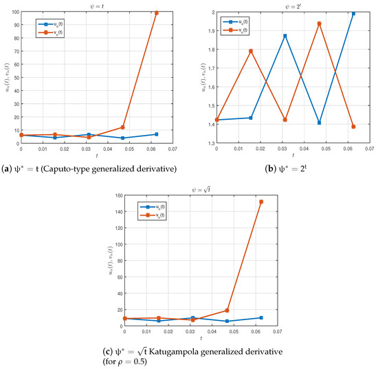
Table 1 and Table 2 show these results. One can see the 2D line plots of ${\underline{\varrho }}_n\left(\mathrm{t}\right)$ and ${\overline{\varrho }}_n\left(\mathrm{t}\right)$ for the ${\mathsf{\psi }}_1^{*}\left(\mathrm{t}\right)=\mathrm{t}$ Caputo derivative, ${\mathsf{\psi }}_2^{*}\left(\mathrm{t}\right)=2^{\mathrm{t}}$, and the ${\mathsf{\psi }}_3^{*}\left(\mathrm{t}\right)=\sqrt{\mathrm{t}}$ Katugampola derivative (for $\rho =0.5$) in Figure 1a,b. In addition, assumption $\left(H2\right)$ is clearly satisfied.

Figure 1. Graphical representation of ${\underline{\varrho }}_n\left(\mathrm{t}\right)$ and ${\overline{\varrho }}_n\left(\mathrm{t}\right)$ in (a) and (b) respectively for the ${\mathsf{\psi }}_1^{*}\left(\mathrm{t}\right)=\mathrm{t}$ Caputo derivative, ${\mathsf{\psi }}_2^{*}\left(\mathrm{t}\right)=2^{\mathrm{t}}$, and the ${\mathsf{\psi }}_3^{*}\left(\mathrm{t}\right)=\sqrt{\mathrm{t}}$ Katugampola derivative (for $\rho =0.5$) in Example 1.

Thus, by Theorem 2, it follows that problem (21) has extremal solutions ${\underline{\varrho }}_{*}$, ${\overline{\varrho }}^{*}\in [0,1+2\mathrm{t}]$, which can be found by means of the iterative sequences $\left\{{\underline{\varrho }}_n\right\}$ and $\left\{{\overline{\varrho }}_n\right\}$ defined by (17) and (18), respectively, as follows:

$$\begin{array}{cc}\hfill {\underline{\varrho }}_{n+1}\left(\mathrm{t}\right)& ={\mathbb{I}}_{{\mathrm{t}}_1^{+}}^{\sigma ;{\mathsf{\psi }}^{*}}\mathcal{V}(\mathrm{t},{\underline{\varrho }}_n\left(\mathrm{t}\right))+\frac{1}{\Lambda }\left(\lambda {\mathbb{I}}_{{\mathrm{t}}_1^{+}}^{\sigma +\nu ;{\mathsf{\psi }}^{*}}\mathcal{V}(\eta ,{\underline{\varrho }}_n\left(\eta \right))+\delta \right)\hfill \\ \hfill & ={\mathbb{I}}_{0^{+}}^{\frac{1}{4};{\mathsf{\psi }}^{*}}\left(2\mathrm{t}-{\left({\underline{\varrho }}_n\left(\mathrm{t}\right)\right)}^2+1\right)+\frac{1}{\Lambda }\left[\frac{3}{4}{\mathbb{I}}_{{\mathrm{t}}_1^{+}}^{\frac{3}{4};{\mathsf{\psi }}^{*}}\left(\frac{4}{3}-{\left({\underline{\varrho }}_n\left(\eta \right)\right)}^2+1\right)+\frac{1}{2}\right]\hfill \end{array}$$

and

$$\begin{array}{cc}\hfill {\overline{\varrho }}_{n+1}\left(\mathrm{t}\right)& ={\mathbb{I}}_{{\mathrm{t}}_1^{+}}^{\sigma ;{\mathsf{\psi }}^{*}}\mathcal{V}(\mathrm{t},{\overline{\varrho }}_n\left(\mathrm{t}\right))+\frac{1}{\Lambda }\left(\lambda {\mathbb{I}}_{{\mathrm{t}}_1^{+}}^{\sigma +\nu ;{\mathsf{\psi }}^{*}}\mathcal{V}(\eta ,{\overline{\varrho }}_n\left(\eta \right))+\delta \right)\hfill \\ \hfill & ={\mathbb{I}}_{0^{+}}^{\frac{1}{4};{\mathsf{\psi }}^{*}}\left(2\mathrm{t}-{\left({\overline{\varrho }}_n\left(\mathrm{t}\right)\right)}^2+1\right)+\frac{1}{\Lambda }\left[\frac{3}{4}{\mathbb{I}}_{{\mathrm{t}}_1^{+}}^{\frac{3}{4};{\mathsf{\psi }}^{*}}\left(\frac{4}{3}-{\left({\overline{\varrho }}_n\left(\eta \right)\right)}^2+1\right)+\frac{1}{2}\right]\hfill \end{array}$$

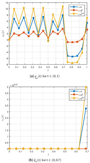
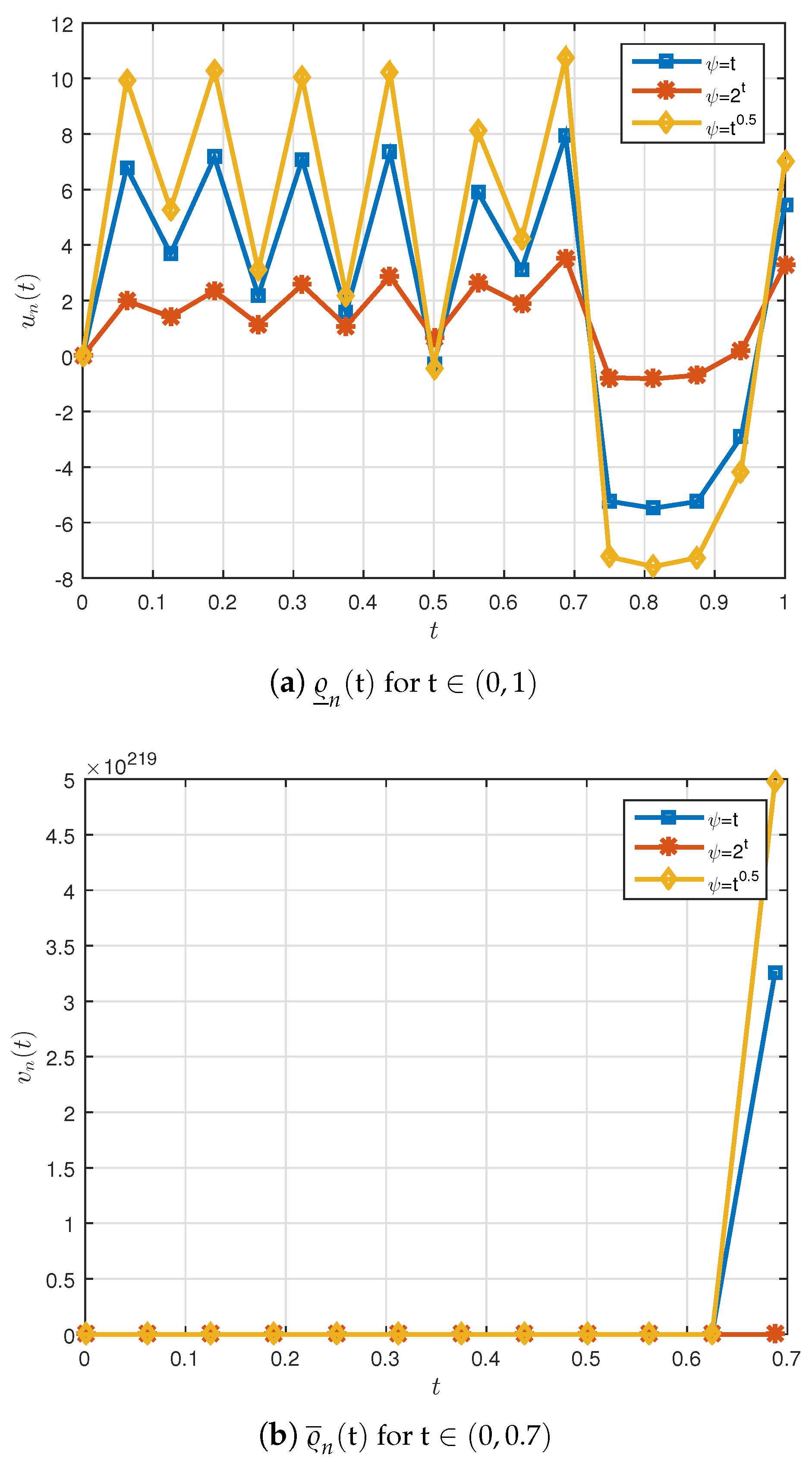
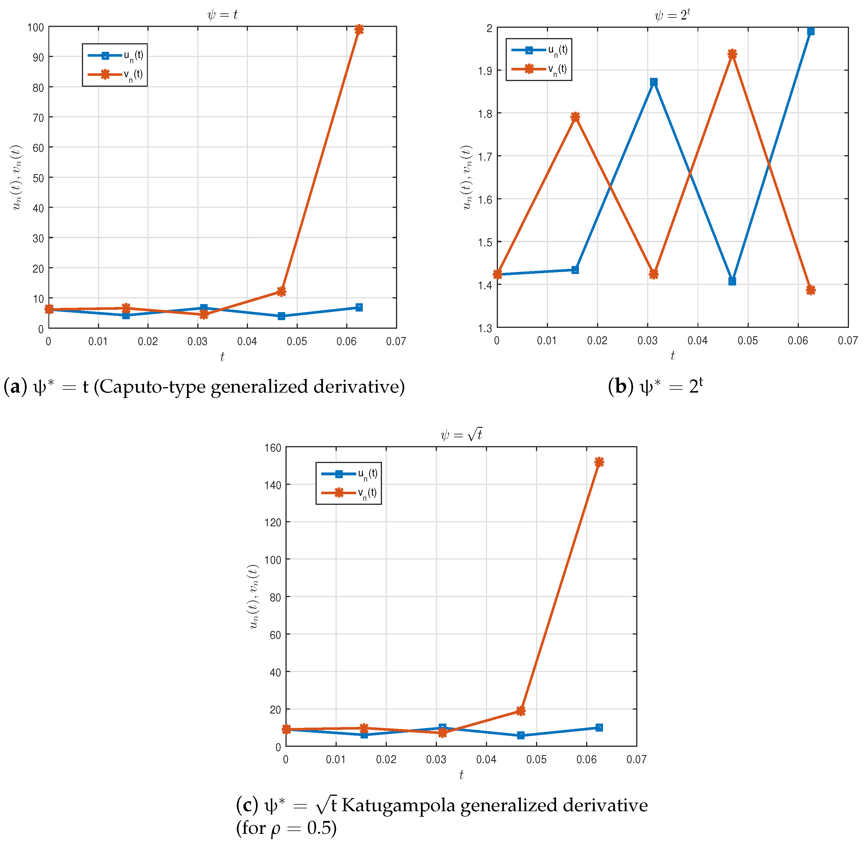
One can see the 2D line plots of ${\underline{\varrho }}_n\left(\mathrm{t}\right)$ and ${\overline{\varrho }}_n\left(\mathrm{t}\right)$ for the ${\mathsf{\psi }}_1^{*}\left(\mathrm{t}\right)=\mathrm{t}$ Caputo derivative, ${\mathsf{\psi }}_2^{*}\left(\mathrm{t}\right)=2^{\mathrm{t}}$, and the ${\mathsf{\psi }}_3^{*}\left(\mathrm{t}\right)=\sqrt{\mathrm{t}}$ Katugampola derivative (for $\rho =0.5$) in Figure 2a–c. Appendix A Algorithm A4 shows how to calculate ${\underline{\varrho }}_n\left(\mathrm{t}\right)$ and ${\overline{\varrho }}_n\left(\mathrm{t}\right)$ for $\mathrm{t}\in ı$.

Figure 2. Graphical representation of ${\underline{\varrho }}_n\left(\mathrm{t}\right)$ and ${\overline{\varrho }}_n\left(\mathrm{t}\right)$ in (a), (b) and (c) respectively for the ${\mathsf{\psi }}_1^{*}\left(\mathrm{t}\right)=\mathrm{t}$ Caputo derivative, ${\mathsf{\psi }}_2^{*}\left(\mathrm{t}\right)=2^{\mathrm{t}}$, and the ${\mathsf{\psi }}_3^{*}\left(\mathrm{t}\right)=\sqrt{\mathrm{t}}$ Katugampola derivative (for $\rho =0.5$) and $\mathrm{t}\in (0,0.07)$ in Example 1.

Example 2.

Consider the following problem:

$$\left\{\begin{array}{cc}{}^C{\mathbb{D}}_{0^{+}}^{\frac{3}{5},{\mathsf{\psi }}^{*}}\varrho \left(\mathrm{t}\right)=2\mathrm{t}-{\varrho }^2\left(\mathrm{t}\right)+1,\hfill & \mathrm{t}\in ı:=[0.1,1.5],\hfill \\ \varrho \left(0\right)=\frac{5}{6}{\mathbb{I}}_{0^{+}}^{\frac{2}{3}}\varrho \left(\frac{3}{7}\right)+\frac{4}{5},\hfill \end{array}\right.$$

(22)

where

$$\sigma =\frac{3}{5}\in (0,1],\nu =\frac{2}{3},\lambda =\frac{5}{6},\eta =\frac{6}{7}\in (0,1),\delta =\frac{9}{11},{\mathrm{t}}_1=0.1,{\mathrm{t}}_2=1.5,$$

and $\mathcal{V}:ı\times \mathbb{R}\to \mathbb{R}$ is given by

$$\mathcal{V}(\mathrm{t},\varrho )=0.6\mathrm{t}-{\varrho }^2+8.5,$$

for $\mathrm{t}\in ı$, $\varrho \in \mathbb{R}$. We take ${\underline{\varrho }}_0\left(\mathrm{t}\right)=0.1$ as the l-solution and ${\overline{\varrho }}_0\left(\mathrm{t}\right)=1.1+\sqrt{\mathrm{t}}$ as the u-solution of problem (21), and we take ${\underline{\varrho }}_0\le {\overline{\varrho }}_0$ for $\mathrm{t}\in ȷ$. So, $\left(H1\right)$ of Theorem 2 holds. Now, we consider three cases for ${\mathsf{\psi }}^{*}$:

$${\mathsf{\psi }}_1^{*}\left(\mathrm{t}\right)=\mathrm{t},{\mathsf{\psi }}_2^{*}\left(\mathrm{t}\right)=2^{\mathrm{t}},{\mathsf{\psi }}_3^{*}\left(\mathrm{t}\right)=\sqrt{\mathrm{t}}.$$

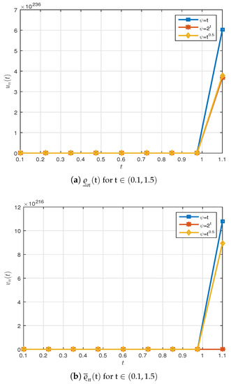
Note that ${\mathsf{\psi }}_1^{*}\left(\mathrm{t}\right)=\mathrm{t}$ and ${\mathsf{\psi }}_3^{*}\left(\mathrm{t}\right)=\sqrt{\mathrm{t}}$ give the Caputo and Katugampola (for $\rho =0.5)$ derivatives in this example. These results are plotted in Figure 3a,b.

Figure 3. Graphical representation of ${\underline{\varrho }}_n\left(\mathrm{t}\right)$ and ${\overline{\varrho }}_n\left(\mathrm{t}\right)$ in (a) and (b) respectively for the ${\mathsf{\psi }}_1^{*}\left(\mathrm{t}\right)=\mathrm{t}$ Caputo derivative, ${\mathsf{\psi }}_2^{*}\left(\mathrm{t}\right)=2^{\mathrm{t}}$, and the ${\mathsf{\psi }}_3^{*}\left(\mathrm{t}\right)=\sqrt{\mathrm{t}}$ Katugampola derivative (for $\rho =0.5$) in Example 2.

With the data provided, we can see from assumption $\left(H3\right)$ that

$$\begin{array}{cc}\hfill \frac{\lambda }{\Gamma (\nu +1)}{({\mathsf{\psi }}^{*}\left(\eta \right)-{\mathsf{\psi }}^{*}\left({\mathrm{t}}_1\right))}^{\nu }& =\frac{\frac{5}{6}}{\Gamma \left(\frac{2}{3}+1\right)}{\left({\mathsf{\psi }}^{*}\left(\frac{6}{7}\right)-{\mathsf{\psi }}^{*}\left(0.1\right)\right)}^{\frac{2}{3}}\hfill \\ \hfill & =\left\{\begin{array}{cc}\frac{\frac{5}{6}}{\Gamma \left(\frac{5}{3}\right)}{\left(\frac{6}{7}-0.1\right)}^{\frac{1}{2}}\approx 0.766841<1,\hfill & {\mathsf{\psi }}^{*}\left(\mathrm{t}\right)=\mathrm{t}.\hfill \\ \frac{\frac{3}{4}}{\Gamma \left(\frac{3}{2}\right)}{\left(2^{\frac{2}{3}}-1\right)}^{\frac{1}{2}}\approx 0.755000<1,\hfill & {\mathsf{\psi }}^{*}\left(\mathrm{t}\right)=2^{\mathrm{t}}.\hfill \\ \frac{\frac{3}{4}}{\Gamma \left(\frac{3}{2}\right)}{\left(\sqrt{\frac{2}{3}}\right)}^{\frac{1}{2}}\approx 0.663661<1,\hfill & {\mathsf{\psi }}^{*}\left(\mathrm{t}\right)=\sqrt{\mathrm{t}}\hfill \end{array}\right.\hfill \end{array}$$

Table 3 and Table 4 show these results. One can see the 2D line plots of ${\underline{\varrho }}_n\left(\mathrm{t}\right)$ and ${\overline{\varrho }}_n\left(\mathrm{t}\right)$ for the ${\mathsf{\psi }}_1^{*}\left(\mathrm{t}\right)=\mathrm{t}$ Caputo derivative, ${\mathsf{\psi }}_2^{*}\left(\mathrm{t}\right)=2^{\mathrm{t}}$, and the ${\mathsf{\psi }}_3^{*}\left(\mathrm{t}\right)=\sqrt{\mathrm{t}}$ Katugampola derivative (for $\rho =0.5$) in Figure 3a,b. Further, assumption $\left(H2\right)$ is clearly satisfied. Thus, by Theorem 2, it follows that problem (22) has extremal solutions ${\varrho }_{*}$, ${\varrho }^{*}\in [0.1,1.1+\sqrt{\mathrm{t}}]$, which can be found by means of the iterative sequences $\left\{{\underline{\varrho }}_n\right\}$ and $\left\{{\overline{\varrho }}_n\right\}$ defined by (17) and (18), respectively, as follows:

$$\begin{array}{cc}\hfill {\underline{\varrho }}_{n+1}\left(\mathrm{t}\right)& ={\mathbb{I}}_{{\mathrm{t}}_1^{+}}^{\sigma ;{\mathsf{\psi }}^{*}}\mathcal{V}(\mathrm{t},{\underline{\varrho }}_n\left(\mathrm{t}\right))+\frac{1}{\Lambda }\left(\lambda {\mathbb{I}}_{{\mathrm{t}}_1^{+}}^{\sigma +\nu ;{\mathsf{\psi }}^{*}}\mathcal{V}(\eta ,{\underline{\varrho }}_n\left(\eta \right))+\delta \right)\hfill \\ \hfill & ={\mathbb{I}}_{{\mathrm{t}}_1^{+}}^{\sigma ;{\mathsf{\psi }}^{*}}\left(2\mathrm{t}-{\left({\underline{\varrho }}_n\left(\mathrm{t}\right)\right)}^2+1\right)+\frac{1}{\Lambda }\left[\lambda {\mathbb{I}}_{{\mathrm{t}}_1^{+}}^{\sigma +\nu ;{\mathsf{\psi }}^{*}}\left(2\eta -{\left({\underline{\varrho }}_n\left(\eta \right)\right)}^2+1\right)+\delta \right]\hfill \end{array}$$

and

$$\begin{array}{cc}\hfill {\underline{\varrho }}_{n+1}\left(\mathrm{t}\right)& ={\mathbb{I}}_{{\mathrm{t}}_1^{+}}^{\sigma ;{\mathsf{\psi }}^{*}}\mathcal{V}(\mathrm{t},{\overline{\varrho }}_n\left(\mathrm{t}\right))+\frac{1}{\Lambda }\left(\lambda {\mathbb{I}}_{{\mathrm{t}}_1^{+}}^{\sigma +\nu ;{\mathsf{\psi }}^{*}}\mathcal{V}(\eta ,{\overline{\varrho }}_n\left(\eta \right))+\delta \right)\hfill \\ \hfill & ={\mathbb{I}}_{{\mathrm{t}}_1^{+}}^{\sigma ;{\mathsf{\psi }}^{*}}\left(2\mathrm{t}-{\left({\overline{\varrho }}_n\left(\mathrm{t}\right)\right)}^2+1\right)+\frac{1}{\Lambda }\left(\lambda {\mathbb{I}}_{{\mathrm{t}}_1^{+}}^{\sigma +\nu ;{\mathsf{\psi }}^{*}}\left(2\eta +{\left({\overline{\varrho }}_n\left(\eta \right)\right)}^2+1\right)+\delta \right).\hfill \end{array}$$

Table 3. Numerical results of ${\underline{\varrho }}_n$ for ${\mathsf{\psi }}^{*}\left(\mathrm{t}\right)=\mathrm{t},2^{\mathrm{t}},\sqrt{\mathrm{t}}$ in Example 2.

		${\underline{\mathit{\varrho }}}_{\mathit{n}}$
$\mathit{n}$	$\mathrm{t}$	${\mathsf{\psi }}^{*}\left(\mathrm{t}\right)=\mathrm{t}$	${\mathsf{\psi }}^{*}\left(\mathrm{t}\right)={\mathbf{2}}^{\mathrm{t}}$	${\mathsf{\psi }}^{*}\left(\mathrm{t}\right)=\sqrt{\mathrm{t}}$
1	$0.10000$	$23.0887$	$21.4299$	$12.7468$
2	$0.22500$	$01.7027\times {10}^2$	$01.3640\times {10}^2$	$01.0319\times {10}^2$
3	$0.35000$	$01.3185\times {10}^4$	$99.6965\times {10}^2$	$82.2118\times {10}^2$
4	$0.47500$	$68.0783\times {10}^6$	$49.0307\times {10}^6$	$42.9176\times {10}^6$
5	$0.60000$	$17.1314\times {10}^{14}$	$11.8461\times {10}^{14}$	$10.8451\times {10}^{14}$
6	$0.72500$	$01.0361\times {10}^{30}$	$69.1495\times {10}^{28}$	$65.6348\times {10}^{28}$
7	$0.85000$	$36.4361\times {10}^{58}$	$23.5622\times {10}^{58}$	$23.0527\times {10}^{58}$
8	$0.97500$	$04.3535\times {10}^{118}$	$02.7357\times {10}^{118}$	$02.7475\times {10}^{118}$
9	$1.10000$	$06.0253\times {10}^{236}$	$03.6879\times {10}^{236}$	$03.7901\times {10}^{236}$
10	$1.22500$	$NaN$	$NaN$	$NaN$
11	$1.35000$	$NaN$	$NaN$	$NaN$
12	$1.47500$	$NaN$	$NaN$	$NaN$

Table 4. Numerical results of ${\overline{\varrho }}_n$ for ${\mathsf{\psi }}^{*}\left(\mathrm{t}\right)=\mathrm{t},2^{\mathrm{t}},\sqrt{\mathrm{t}}$ in Example 2.

		${\overline{\mathit{\varrho }}}_{\mathit{n}}$
$\mathit{n}$	$\mathrm{t}$	${\mathsf{\psi }}^{*}\left(\mathrm{t}\right)=\mathrm{t}$	${\mathsf{\psi }}^{*}\left(\mathrm{t}\right)={\mathbf{2}}^{\mathrm{t}}$	${\mathsf{\psi }}^{*}\left(\mathrm{t}\right)=\sqrt{\mathrm{t}}$
1	$0.10000$	$23.0887$	$21.4299$	$12.7468$
2	$0.22500$	$01.1374\times {10}^2$	$90.2639$	$69.2844$
3	$0.35000$	$58.6017\times {10}^2$	$43.0855\times {10}^2$	$37.2431\times {10}^2$
4	$0.47500$	$13.6661\times {10}^6$	$09.1617\times {10}^6$	$08.9616\times {10}^6$
5	$0.60000$	$71.6666\times {10}^{12}$	$41.3606\times {10}^{12}$	$49.1158\times {10}^{12}$
6	$0.72500$	$20.3287\times {10}^{26}$	$08.4297\times {10}^{26}$	$15.0160\times {10}^{26}$
7	$0.85000$	$02.0382\times {10}^{54}$	$35.0156\times {10}^{52}$	$01.6593\times {10}^{54}$
8	$0.97500$	$03.2721\times {10}^{108}$	$06.0417\times {10}^{106}$	$02.7695\times {10}^{108}$
9	$1.10000$	$10.7866\times {10}^{216}$	$17.9871\times {10}^{212}$	$08.9489\times {10}^{216}$
10	$1.22500$	$NaN$	$NaN$	$NaN$
11	$1.35000$	$NaN$	$NaN$	$NaN$
12	$1.47500$	$NaN$	$NaN$	$NaN$

One can see the 2D line plots of ${\underline{\varrho }}_n\left(\mathrm{t}\right)$ and ${\overline{\varrho }}_n\left(\mathrm{t}\right)$ for the ${\mathsf{\psi }}_1^{*}\left(\mathrm{t}\right)=\mathrm{t}$ Caputo derivative, ${\mathsf{\psi }}_2^{*}\left(\mathrm{t}\right)=2^{\mathrm{t}}$, ${\mathsf{\psi }}_3^{*}\left(\mathrm{t}\right)=\sqrt{\mathrm{t}}$, and the Katugampola derivative (for $\rho =0.5$) in Figure 3a,b. Appendix A Algorithm A4 shows how to calculate ${\underline{\varrho }}_n\left(\mathrm{t}\right)$ and ${\overline{\varrho }}_n\left(\mathrm{t}\right)$ for $\mathrm{t}\in ı$.

5. Conclusions

In this study, we investigated the existence of solutions for a nonlinear FDE in the frame of the $\mathsf{\psi }-$Caputo derivative with integral boundary conditions. To prove the main theorems, the monotone iterative and the upper–lower solution techniques in the sense of the $\mathsf{\psi }-$Caputo fractional operator were used. Based on certain conditions, we constructed $mis$ that uniformly converged to the extremal solutions of BVP. The results were tested by constructing two equations corresponding to BVP (3). Different values for $\mathsf{\psi }$, such as the ${\mathsf{\psi }}^{*}\left(\mathrm{t}\right)=\mathrm{t}$, Caputo, ${\mathsf{\psi }}^{*}\left(\mathrm{t}\right)=2^{\mathrm{t}}$, ${\mathsf{\psi }}^{*}\left(\mathrm{t}\right)=\sqrt{\mathrm{t}}$, and Katugampola (for $\rho =0.5)$ derivatives and the upper and lower solutions, were examined and illustrated for the purpose of verification. We conclude that the results reported in this paper are of great significance for the relevant audience and can be applied to different types of fractional differential problems.

References

- Hilfer, R. Applications of Fractional Calculus in Physics; World Scientific: Singapore, 2000. [Google Scholar]
- Oldham, K.B. Fractional differential equations in electrochemistry. Adv. Eng. Softw. 2010, 41, 9–12. [Google Scholar] [CrossRef]
- Sabatier, J.; Agrawal, O.P.; Machado, J.A.T. Advances in Fractional Calculus-Theoretical Developments and Applications in Physics and Engineering; Springer: Dordrecht, The Netherlands, 2007. [Google Scholar]
- Tarasov, V.E. Fractional Dynamics: Application of Fractional Calculus to Dynamics of Particles, Fields and Media; Springer Science & Business Media: Berlin/Heidelberg, Germany, 2010. [Google Scholar]
- Kilbas, A.A.; Srivastava, H.; Trujillo, J.J. Theory and Applications of Fractional Differential Equations; Elsevier Science B.V.: Amsterdam, The Netherlands, 2006; Volune 204. [Google Scholar]
- Almeida, R. A Caputo fractional derivative of a function with respect to another function. Commun. Nonlinear Sci. Numer. Simul. 2017, 44, 460–481. [Google Scholar] [CrossRef] [Green Version]
- Alzabut, J.; Selvam, A.G.M.; El-Nabulsi, R.A.; Dhakshinamoorthy, V.; Samei, M.E. Asymptotic Stability of Nonlinear Discrete Fractional Pantograph Equations with Non-Local Initial Conditions. Symmetry 2021, 13, 473. [Google Scholar] [CrossRef]
- Almeida, R.; Malinowska, A.B.; Monteiro, M.T.T. Fractional differential equations with a Caputo derivative with respect to a kernel function and their applications. Math. Meth. Appl. Sci. 2018, 41, 336–352. [Google Scholar] [CrossRef] [Green Version]
- Almeida, R.; Jleli, M.; Samet, B. A numerical study of fractional relaxation-oscillation equations involving ψ-Caputo fractional derivative. Rev. R. Acad. Cienc. Exactas Fís. Nat. Ser. A Mat. RACSAM 2019, 113, 1873–1891. [Google Scholar] [CrossRef]
- Baitiche, Z.; Derbazi, C.; Alzabut, J.; Samei, M.E.; Kaabar, M.K.A.; Siri, Z. Monotone Iterative Method for Langevin Equation in Terms of ψ-Caputo Fractional Derivative and Nonlinear Boundary Conditions. Fractal Fract. 2021, 5, 81. [Google Scholar] [CrossRef]
- Samei, M.; Hedayati, V.; Rezapour, S. Existence results for a fraction hybrid differential inclusion with Caputo-Hadamard type fractional derivative. Adv. Differ. Equations 2019, 2019, 163. [Google Scholar] [CrossRef]
- Adjabi, Y.; Samei, M.E.; Matar, M.M.; Alzabut, J. Langevin differential equation in frame of ordinary and Hadamard fractional derivatives under three point boundary conditions. AIMS Math. 2021, 6, 2796–2843. [Google Scholar] [CrossRef]
- Samet, B.; Aydi, H. Lyapunov-type inequalities for an anti-periodic fractional boundary value problem involving ψ-Caputo fractional derivative. J. Inequal. Appl. 2018, 2018, 286. [Google Scholar] [CrossRef] [Green Version]
- Abdo, M.S.; Panchal, S.K.; Saeed, A.M. Fractional boundary value problem with ψ-Caputo fractional derivative. Proc. Math. Sci. 2019, 129, 14. [Google Scholar] [CrossRef]
- Abbas, S.; Benchohra, M.; N’Guŕékata, G.M. Topics in Fractional Differential Equations; Springer: New York, NY, USA, 2015. [Google Scholar]
- Miller, K.S.; Ross, B. An Introduction to Fractional Calculus and Fractional Differential Equations; Academic Press: New York, NY, USA, 1993. [Google Scholar]
- Podlubny, I. Fractional Differential Equations; Academic Press: San Diego, CA, USA, 1999. [Google Scholar]
- Zhou, Y. Basic Theory of Fractional Differential Equations; World Scientific: Singapore, 2014. [Google Scholar]
- Agarwal, R.P.; Benchohra, M.; Hamani, S. A survey onexistence results for boundary value problems of nonlinear fractional differential equations and inclusions. Acta Appl. Math. 2010, 109, 973–1033. [Google Scholar] [CrossRef]
- Benchohra, M.; Graef, J.R.; Hamani, S. Existence results for boundary value problems with non-linear fractional differential equations. Appl. Anal. 2008, 87, 851–863. [Google Scholar] [CrossRef]
- Abbas, S.; Benchohra, M.; Hamidi, N.; Henderson, J. Caputo–Hadamard fractional differential equations in Banach spaces. Fract. Calc. Appl. Anal. 2018, 21, 1027–1045. [Google Scholar] [CrossRef]
- Boutiara, A.; Guerbati, K.; Benbachir, M. Caputo-Hadamard fractional differential equation with three-point boundary conditions in Banach spaces. AIMS Math. 2020, 5, 259–272. [Google Scholar]
- Aghajani, A.; Pourhadi, E.; Trujillo, J.J. Application of measure of noncompactness to a Cauchy problem for fractional differential equations in Banach spaces. Fract. Calc. Appl. Anal. 2013, 16, 962–977. [Google Scholar] [CrossRef]
- Kucche, K.D.; Mali, A.D.; Sousa, J.V.C. On the nonlinear Ψ-Hilfer fractional differential equations. Comput. Appl. Math. 2019, 38, 25. [Google Scholar] [CrossRef]
- Zhang, L.; Ahmad, B.; Wang, G. Explicit iterations and extremal solutions for fractional differential equations with nonlinear integral boundary conditions. Appl. Math. Comput. 2015, 268, 388–392. [Google Scholar] [CrossRef]
- Derbazi, C.; Baitiche, Z.; Benchohra, M.; Cabada, A. Initial Value Problem For Nonlinear Fractional Differential Equations With ψ-Caputo Derivative Via Monotone Iterative Technique. Axioms 2020, 9, 57. [Google Scholar] [CrossRef]
- Ali, S.; Shah, K.; Jarad, F. On stable iterative solutions for a class of boundary value problem of nonlinear fractional order differential equations. Math. Methods Appl. Sci. 2019, 42, 969–981. [Google Scholar] [CrossRef]
- Al-Refai, M.; Hajji, M.A. Monotone iterative sequences for nonlinear boundary value problems of fractional order. Nonlinear Anal. 2011, 74, 3531–3539. [Google Scholar] [CrossRef]
- Alsaedi, A.; Ahmad, B.; Alghanmi, M. Extremal solutions for generalized Caputo fractional differential equations with Steiltjes-type fractional integro-initial conditions. Appl. Math. Lett. 2019, 91, 113–120. [Google Scholar] [CrossRef]
- Chen, C.; Bohner, M.; Jia, B. Method of upper and lower solutions for nonlinear Caputo fractional difference equations and its applications. Fract. Calc. Appl. Anal. 2019, 22, 1307–1320. [Google Scholar] [CrossRef]
- Dhaigude, D.; Rizqan, B. Existence and uniqueness of solutions of fractional differential equations with deviating arguments under integral boundary conditions. Kyungpook Math. J. 2019, 59, 191–202. [Google Scholar]
- Fazli, H.; Sun, H.; Aghchi, S. Existence of extremal solutions of fractional Langevin equation involving nonlinear boundary conditions. Int. J. Comput. Math. 2020, 2020, 1720662. [Google Scholar] [CrossRef]
- Lin, X.; Zhao, Z. Iterative technique for a third-order differential equation with three-point nonlinear boundary value conditions. Electron. J. Qual. Theory Differ. Equ. 2016, 12, 10. [Google Scholar] [CrossRef]
- Mao, J.; Zhao, Z.; Wang, C. The unique iterative positive solution of fractional boundary value problem with q-difference. Appl. Math. Lett. 2020, 100, 106002. [Google Scholar] [CrossRef]
- Meng, S.; Cui, Y. The extremal solution to conformable fractional differential equations involving integral boundary condition. Mathematics 2019, 7, 186. [Google Scholar] [CrossRef] [Green Version]
- Wang, G.; Sudsutad, W.; Zhang, L.; Tariboon, J. Monotone iterative technique for a nonlinear fractional q-difference equation of Caputo type. Adv. Diff. Equ. 2016, 2016, 211. [Google Scholar] [CrossRef] [Green Version]
- Zhang, S. Monotone iterative method for initial value problem involving Riemann-Liouville fractional derivatives. Nonlinear Anal. 2009, 71, 2087–2093. [Google Scholar] [CrossRef]
- Eswari, R.; Alzabut, J.; Samei, M.E.; Zhou, H. On periodic solutions of a discrete Nicholson’s dual system with density-dependent mortality and harvesting terms. Adv. Differ. Equations 2021, 2021, 360. [Google Scholar] [CrossRef]
Publisher’s Note: MDPI stays neutral with regard to jurisdictional claims in published maps and institutional affiliations. |
© 2021 by the authors. Licensee MDPI, Basel, Switzerland. This article is an open access article distributed under the terms and conditions of the Creative Commons Attribution (CC BY) license (https://creativecommons.org/licenses/by/4.0/).