Avoiding Dynamical Degradation in Computer Simulation of Chaotic Systems Using Semi-Explicit Integration: Rössler Oscillator Case

Abstract

Dynamical degradation is a known problem in the computer simulation of chaotic systems. Data type limitations, sampling, and rounding errors give rise to the periodic behavior. In applications of chaotic systems in secure communication and cryptography systems, such effects can reduce data storage security and operation. In this study, we considered a possible solution to this problem by using semi-explicit integration. The key idea is to perturb the chaotic trajectory by switching between two integrators, which possess close but still different numerical solutions. Compared with the traditional approach based on the perturbation of the bifurcation parameter, this technique does not significantly change the nonlinear properties of the system. We verify the efficiency of the proposed perturbation method through several numerical experiments using the well-known Rössler oscillator.

1. Introduction

In recent decades, chaotic systems have been widely used in many engineering and scientific tasks, including secure communication [1,2,3,4], neural networks [5,6], watermarking [7], cryptography [8,9,10], robotics [11,12], sensors [13], signal processing [14], etc. Usually, such practically oriented studies and applications are performed using computer simulation. Converting mathematical models to executable ones inevitably causes an imprecision. In addition to the identification error of the mathematical model, the discrepancy between the numerical results and the prototype behavior is enhanced by the data type precision, discretization methods error, and round-off results of arithmetic operations [15]. In chaotic systems, the combination of these factors can lead to the degradation of chaotic dynamics [16]. In [17], K.J. Persohn and R.J. Povinelli explicitly demonstrated that for four-bit binary fractions representation, the trajectory of the known logistic map starts repeating after two iterations with a period of three for any initial value.

Several methods have been proposed to avoid cycles in the chaotic trajectories obtained in computer simulations [16,18,19,20,21,22,23,24,25]. One of the most straightforward and easily implementable approaches is perturbing the trajectory of a discrete chaotic system or the bifurcation parameter [16,18,19,20]. Usually, the cycle breaking is performed using an auxiliary discrete chaotic map of a small dimension. A significant period prolongation with this technique was demonstrated for delayed chaotic maps [21]. To determine the disturbance moments, a linear feedback shift register (LFSR) or a chaotic analog system can be used [22,23,24]. In [25], it was proposed to introduce perturbation only when the trajectory becomes a loop. This approach requires additional memory.

All of the above approaches effectively cope with the period increasing of the trajectory of a chaotic system in long-term simulation. These techniques are especially useful in cryptographic applications of chaotic systems [21,24]. The security of chaos-based algorithms often depends on the degree of randomness of the binary sequences generated from the numerical orbits [26]. However, all considered techniques can significantly influence the properties of the chaotic system. Switching the bifurcation parameter can lead to a change in the oscillations’ patterns. Due to the perturbation of the state variable, a leaving of the attractor can occur. At the same time, problems with the long-term simulation of chaotic systems with constant parameters often arise. For example, some metrics, including the largest Lyapunov exponent, are reliably calculated only over a large time interval [27,28,29]. Moreover, the study of chimera states in ensembles of coupled oscillators also implies long-term simulation [30]. In both cases, the considered techniques for avoiding dynamical degradation can distort the results of the analysis. Such methods are not applicable for synchronization-based communication systems since any perturbation violates the identity of the oscillations generated by the receiver and transmitter. It can take a long time for the sync state to recover [31]. Thus, the development of new approaches to reduce dynamic degradation is of practical interest.

In this study, we propose to use the specific properties of semi-implicit integrators as a possible solution to the problem of extending the chaotic sequence. Instead of perturbing the nonlinearity parameter, we consider switching between two finite-difference schemes obtained by semi-explicit integration for a particular chaotic system. We use a pair of Euler–Cromer methods with the forward and backward order of state variables calculation, which produce similar but still different enough Taylor series. In this case, the calculation error for each state variable changes due both to a different order of arithmetic operations and an errors discrepancy in the numerical methods when the integrator is switched. Our experiments showed that this technique makes it possible to increase the period of chaotic behavior significantly. Moreover, the proposed method can be effectively implemented in embedded chaos-based communication systems since it can incorporate a single finite-difference scheme with different connections between arithmetic modules operated by logic gates.

Thus, the main contribution of this study can be formulated as follows:

• the new technique for extending the period of chaotic sequences is given;
• the proposed method does not introduce additional perturbations to the chaotic oscillations in comparison with traditional methods based on switching nonlinearity parameters;
• the considered approach can be implemented in embedded systems without using additional hardware resources.

The rest of the paper is organized as follows. Section 2 describes the proposed technique and shows how it can be applied to the sample chaotic system. Section 3 presents the algorithm for detecting cycles in numerical sequences. We experimentally investigated the proposed method in comparison with a common technique based on parameter switching. Finally, some conclusions and discussions are given in Section 4.

2. Materials and Methods

A common practice for avoiding cycles in the trajectories of a chaotic system in computer simulations is switching the values of the bifurcation parameters. In this approach, two main factors prevent looping. First, the steady-state oscillation mode can be violated, and an undesirable situation can arise when the trajectory leaves the attractor or the chaotic behavior changes to a periodic mode. The second aspect concerns floating-point calculations, which involve normalizing numbers in binary operations [32]. Two bifurcation parameter values can be normalized in different ways, which leads to various errors at each integration step. We employed a similar trick of switching between two semi-explicit finite-difference schemes that simulate the same chaotic system in the proposed approach.

Let us consider the idea of semi-explicit integration first.

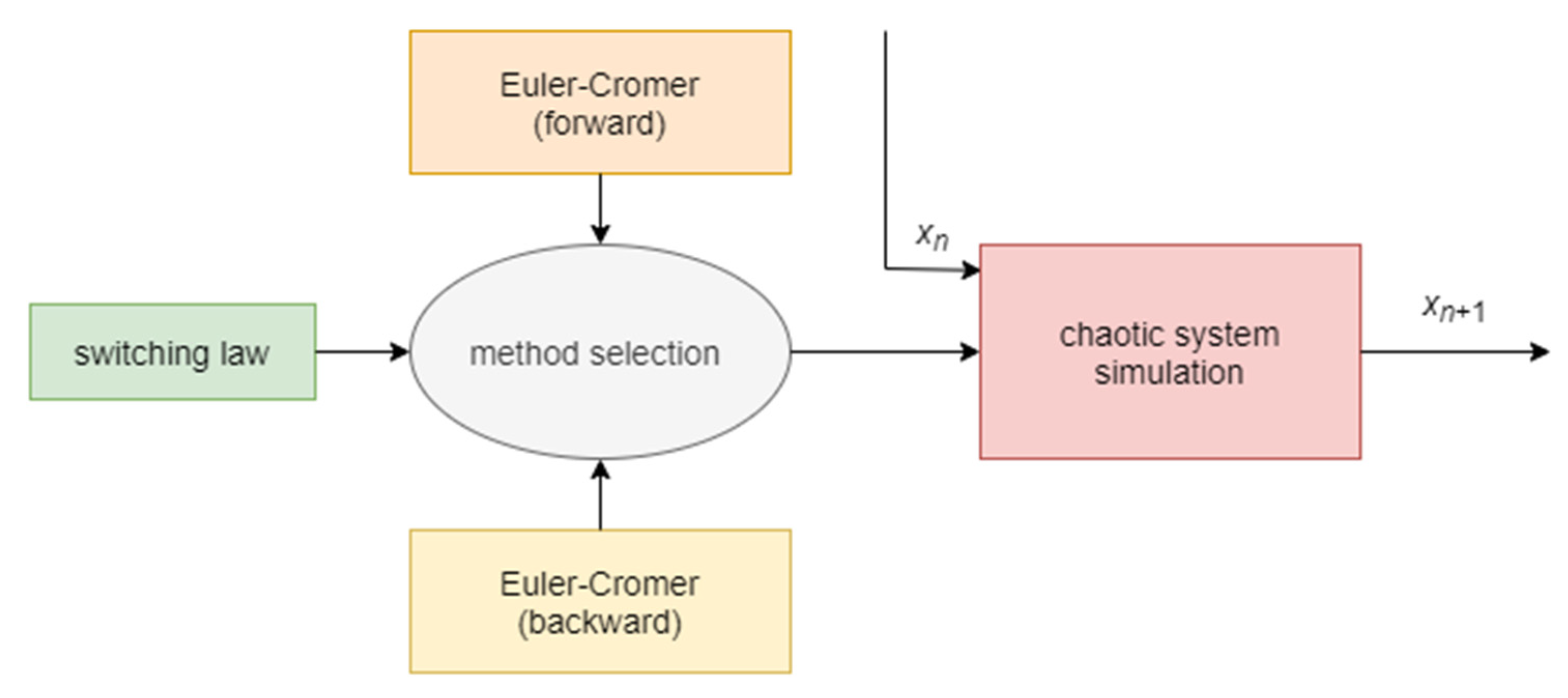
2.1. Semi-Explicit Integration

Semi-implicit integration implies the reuse of already approximated values of state variables at the (n + 1) step to calculate the rest of the state variables within one integration step [32,33]. Being compared with explicit and implicit numerical methods, semi-explicit methods can include additional terms of the Taylor series. The set and number of such expressions depend on the calculation order of the right-hand sides of the equations.

The simplest semi-explicit integration technique is the first-order Euler–Cromer method, also known as the semi-explicit Euler or symplectic Euler method [33,34]. It can be introduced for the two-dimensional Hamiltonian system:

$$\begin{array}{l}\dot{x}=f\left(t,v\right)\\ \dot{v}=g\left(t,x\right)\end{array}$$

(1)

where f and g are given right-hand side functions. The Euler–Cromer method produces an approximate discrete solution for System (1) by iterating:

$$\begin{array}{l}{x}_{n+1}=x_n+hf\left(t_n,v_n\right)\\ v_{n+1}=v_n+hg\left(t_n,x_{n+1}\right)\end{array}$$

(2)

where h is the integration step. The key difference the Euler–Cromer method (2) makes following a conventional explicit Euler method is that the equation for v_n+1 uses an already calculated value of x_n+1. Such calculation inevitably leads to the appearance of an additional term in the Taylor expansion of variable v. If we reverse the order of calculations, we get the modification of the Euler–Cromer method of the same order of accuracy:

$$\begin{array}{l}{v}_{n+1}=v_n+hg\left(t_n,x_n\right)\\ x_{n+1}=x_n+hf\left(t_n,v_{n+1}\right)\end{array}$$

(3)

with an extra term in the Taylor series for variable x. Thus, by changing the sequence of the approximation of the state variables, we can vary the number of additional terms of the Taylor expressions when solving the differential equations of arbitrary order. One can notice that for a system consisting of N equations, in the general case, there are N! variants of finite-difference schemes that can be obtained with the Euler–Cromer (3) integration. Let us consider how one can use this feature of semi-explicit methods to avoid chaotic degradation in discrete simulations of continuous chaotic systems.

2.2. Perturbation Technique

The proposed technique is based on switching between two finite-difference schemes obtained through the Euler–Cromer integration with different calculations. The Taylor series reconstructed by such methods coincide up to the first term but are different in the remaining terms. Therefore, switching between two various schemes obtained via the Euler–Cromer integration can significantly vary the truncation error accumulated on each integration step. In addition to the methodical error, the different order of calculations also introduces some extra perturbation since floating-point operations are not completely associative [32].

Thus, we propose applying the perturbation scheme shown in Figure 1 to avoid the cycles in the computer simulation of chaotic systems. At each integration step, the switching law generates 0 or 1, which corresponds to the choice of the corresponding Euler–Cromer integration method with a certain order of calculations. For example, one can use the forward and backward approximation, as is shown in Figure 1.

To determine the moment of switching, any of the known approaches can be applied, including LFSR or a pseudo-random bit generator (PRBG) [24]. According to the LFSR rule, each finite-difference scheme is matched to the switching law output. Figure 2 represents one of the possible schemes with LFSR given by a primitive polynomial x⁸ + x⁴ + x³ + x + 1 with initial state (0, 0, 0, 0, 0, 0, 0, 1).

It should be noted that the developed perturbation technique can be applied using high-order methods as well, including the semi-implicit composition and extrapolation methods [35,36]. However, in practical applications—e.g., communication systems based on chaotic synchronization phenomenon—it is required to use finite-difference schemes with a minimum number of arithmetic operations [37]. The use of high-order methods in solving such problems leads to a decrease in the data transfer rate. In addition, in embedded systems the dimension of the implemented finite-difference scheme is limited by hardware resources, since multiple chaos generators and receivers are implemented. Therefore, the present study focused on studying methods of a small order of algebraic accuracy that satisfy this criterion.

Let us consider the results of applying the proposed approach to simulate a chaotic system.

3. Experimental Results

As the sample system, we use the well-studied Rössler oscillator [38] described by the following system of ordinary differential equations (ODE):

$$\begin{array}{l}\dot{x}=-y-z\\ \dot{y}=x+ay\\ \dot{z}=b+z\left(x-c\right)\end{array}$$

(4)

where a, b, and c are bifurcation parameters.

Let us consider the finite-difference scheme for System (4) obtained by the Euler–Cromer integration with a straightforward order of state variables calculation:

$$\begin{array}{l}{x}_{n+1}=x_n+h\left(-y_n-z_n\right)\\ y_{n+1}=y_n+h\left(x_{n+1}+a{y}_n\right)\\ z_{n+1}=z_n+h\left(b+z_n\left(x_{n+1}-c\right)\right)\end{array}$$

(5)

Substituting x_n+1 into the other equations and making a cancellation, one can obtain:

$$\begin{array}{l}{x}_{n+1}=x_n+h\left(-y_n-z_n\right)\\ y_{n+1}=y_n+h\left(x_n+a{y}_n\right)+h^2\left(-y_n-z_n\right)\\ z_{n+1}=z_n+h\left(b+z_n\left(x_n-c\right)\right)+h^2{z}_n\left(-y_n-z_n\right)\end{array}$$

(6)

It can be seen from Equation (6) that the solution of System (4) is accurately approximated to the first term of the Taylor series, while the resulting expansions partially contain terms from the rest of the series. Applying the Euler–Cromer method with reverse calculation order, we obtain another finite-difference scheme:

$$\begin{array}{l}{z}_{n+1}=z_n+h\left(b+z_n\left(x_n-c\right)\right)\\ y_{n+1}=y_n+h\left(x_n+a{y}_n\right)\\ x_{n+1}=x_n+h\left(-y_{n+1}-z_{n+1}\right)\end{array}$$

(7)

which can be rewritten as:

$$\begin{array}{l}{z}_{n+1}=z_n+h\left(b+z_n\left(x_n-c\right)\right)\\ y_{n+1}=y_n+h\left(x_n+a{y}_n\right)\\ x_{n+1}=x_n+h\left(-y_n-z_n\right)+h^2\left(-x_n-a{y}_n-b-z_n\left(x_n-c\right)\right)\end{array}$$

(8)

As one can see from Formulas (6) and (8), the reconstructed series coincide up to the first term of the Taylor series but differ in the remaining terms.

3.1. Comparison with Known Perturbation Techniques

In the first experimental part of our study, we compared the proposed approach with known techniques of avoiding cycles in chaotic sequences. First, we considered the widely used method of switching the bifurcation parameter. The second investigated method was changing the order of calculations in the right-hand side function of the differential equations. For example, for System (4), the equation of the z variable can be rewritten as:

$$\begin{array}{l}\dot{x}=-y-z\\ \dot{y}=x+ay\\ \dot{z}=b+zx-zc\end{array}$$

(9)

Nepomuceno et al. found that such a trick in chaotic systems leads to entirely different chaotic trajectories [39]. It is expected that this approach will demonstrate poorer performance than the conventional parameter perturbation and the proposed method. However, this approach can assess the degree of influence of rounding errors of different numbers or the order of operations on the extension of the sequence period.

For the approaches under comparison, the switching moments are determined by the LFSR shown in Figure 2. We estimated the period length of the trajectories of the Rössler oscillator simulated with a 16-bit fixed-point data type with an 8-bit set for the word length. The simulation was performed on time interval T = 300 s and the integration step equaled 0.0117188 s. We considered three sets of initial conditions. Each sample set was generated as follows. We equated one of the initial conditions to 0.96875. The rest of the two initial values were in the range [−0.0315; 0.96875] with an increment of 0.00390625, which coincided with the minimum representable value in the chosen 16-bit fixed-point data type.

In the parameter-perturbation method, switching was performed for parameter b between values 0.1875 and 0.210938, for which chaotic behavior was observed. The approach that is based on a different order of operations uses the original Rössler system (4) and its representation (9). In both cases, simulations were performed by the Euler–Cromer method with the forward order of computation. In the proposed technique, we applied finite-difference schemes (5) and (7), respectively.

To detect cycles’ appearance in chaotic sequences, we used the algorithm described in [40]. The experimental results obtained with the set of initial conditions where y₀ is fixed are given in Figure 3. The number of periodic sequences for the sample set with y₀ = 0.96875 for different perturbation techniques is shown in

Table 1. The number of periodic sequences in the set of initial conditions of size 65,536 for different perturbation techniques when y₀ = 0.96875 and x₀, z₀ $\in$ [−0.0315; 0.96875].

Perturbation Technique	Number of Periodic Sequences
Original 16-bit model	10,038
Switching between two forms of the right-hand side functions	428
Perturbation of the bifurcation parameter	13
Proposed technique	21

. The estimates obtained with the other two sets are presented in Appendix A (Figure A1 and Figure A2). The abscissa and ordinate axes in Figure 3, Figure A1 and Figure A2 correspond to the values of the initial conditions from which the simulation began. Pairs of initial values for which equal numbers were found in the generated sequence are marked black. It can be noted that the number of pairs of initial conditions leading to periodic solutions was reduced for all the considered techniques compared to the original model (case (a) in Figure 3, Figure A1 and Figure A2). The efficiency of the proposed approach was close to the traditional method based on switching the bifurcation parameter (cases (c) and (d) in Figure 3, Figure A1 and Figure A2). In addition, it can be seen that by changing the order of calculations only, one cannot obtain the required period extension (case (b) in Figure 3, Figure A1 and Figure A2). It can be seen that none of the considered techniques disturbed the trajectory enough to change this mode to chaotic behavior.

3.2. Comparison with Other Finite-Difference Schemes

In the second part of the experimental study, we checked whether the perturbation was caused by different additional terms of the Taylor series in switchable semi-explicit schemes. We used the same flowchart shown in Figure 1 but applied other known integration methods, namely the traditional Euler integration, the explicit midpoint method, and the Heun (Runge-Kutta 2) algorithm.

For the sample System (4), the conventional Euler integration gives the following finite-deference scheme:

$$\begin{array}{l}{x}_{n+1}=x_n+h\left(-y_n-z_n\right)\\ y_{n+1}=y_n+h\left(x_n+a{y}_n\right)\\ z_{n+1}=z_n+h\left(b+z_n\left(x_n-c\right)\right)\end{array}$$

(10)

Formula (10) approximates the solution of the Rössler system up to the first term of the Taylor series. In the perturbation technique, the Euler method can be switched with its semi-explicit counterpart.

The explicit midpoint method is a second-order refinement of the explicit Euler method [41]. The finite-difference model obtained by such a technique is as follows:

$$\begin{array}{l}{x}_{n+0.5}=x_n+0.5h\left(-y_n-z_n\right)\\ y_{n+0.5}=y_n+0.5h\left(x_n+a{y}_n\right)\\ z_{n+0.5}=z_n+0.5h\left(b+z_n\left(x_n-c\right)\right)\\ \\ x_{n+1}=x_n+h\left(-y_{n+0.5}-z_{n+0.5}\right)\\ y_{n+1}=y_n+h\left(x_{n+0.5}+a{y}_{n+0.5}\right)\\ z_{n+1}=z_n+h\left(b+z_{n+0.5}\left(x_{n+0.5}-c\right)\right)\end{array}$$

(11)

Another extension of the Euler method is known, called the Heun method [41]. For System (4) it gives the following equations:

$$\begin{array}{l}{x}_{n+1}=x_n+h\left(-y_n-z_n\right)\\ y_{n+1}=y_n+h\left(x_n+a{y}_n\right)\\ z_{n+1}=z_n+h\left(b+z_n\left(x_n-c\right)\right)\\ \\ x_{n+1}=x_n+0.5h\left(\left(-y_n-z_n\right)+\left(-y_{n+1}-z_{n+1}\right)\right)\\ y_{n+1}=y_n+0.5h\left(\left(x_n+a{y}_n\right)+\left(x_{n+1}+a{y}_{n+1}\right)\right)\\ z_{n+1}=z_n+0.5h\left(\left(b+z_n\left(x_n-c\right)\right)+\left(b+z_{n+1}\left(x_{n+1}-c\right)\right)\right)\end{array}$$

(12)

Both methods (11) and (12) are explicit and possess the algebraic accuracy of second order. The finite-difference schemes obtained via these techniques restore the Taylor series precisely up to the second term. Therefore, this pair of methods can potentially be used together to simulate a chaotic system.

It can be assumed that the perturbation can also result from switching methods of different orders. Therefore, as the third case in our comparison, we include Euler and Heun methods.

We repeated the estimate of the period length for the sample set of initial conditions with y₀ = 0.96875 and x₀, z₀$\in$ [−0.0315; 0.96875]. The obtained results are shown in Figure 4. The numbers of sequences with cycles are listed in

Table 2. The number of periodic sequences in the set of initial conditions of size 65,536 for the switching technique based on different finite-difference schemes. y₀ = 0.96875, x₀, z₀$\in$ [−0.0315; 0.96875].

Switchable Methods	Number of Periodic Sequences
Two Euler–Cromer methods	21
Euler–Cromer and Euler methods	1183
Explicit midpoint and Heun methods	2608
Heun and Euler methods	599

.

As one can see, the efficiency of the approach based on methods of different orders was close to the technique based on switching various forms of the right-hand sides of the differential equation. Additional terms of the Taylor series, reconstructed by the Euler–Cromer method, did not provide the same perturbation when paired with the Euler method than with the semi-explicit copy with a different order of calculations. The worst performance was shown by switching between the Heun and the midpoint methods. This can be explained by the relatively low difference between the solutions produced by these second-order integrators. Only the different order of algebraic operations caused the perturbation in this case.

Thus, we can conclude that the best perturbation is provided by switching semi-explicit methods among the approaches considered.

4. Conclusions and Discussion

In this study, a new approach to avoid dynamical degradation in chaotic systems was proposed. It was theoretically predicted that applying a pair of finite-difference schemes obtained by the semi-explicit integration method can help prevent chaotic degradation in the generated sequences. This phenomenon can be explained as follows: slight changes in the truncation errors and round-off errors of arithmetic operations result in simultaneous changes in the discrete system’s trajectory. Experimental results confirmed the theoretical suggestions and showed that it is possible to extend the period of a chaotic sequence by switching the integration order in computations performed with short data types. The efficiency of the proposed approach was comparable to the traditional technique based on the perturbation of the bifurcation parameter. However, an indisputable advantage is the invariability of the bifurcation properties of the model during the perturbation. It can be helpful in various types of analysis that require long-term simulation and secure communication systems, where the concealment of transmission is preferred. In addition, semi-explicit integrators can be compactly implemented in embedded communication systems based on chaotic synchronization. In such systems, to avoid dynamic degradation, in the transmitter, one can switch the input values of the Euler–Cromer integrator as shown in Figure 5, obtaining different orders of calculations. In comparison, for example, from the switching between the explicit midpoint method (11) and the Heun method (12), to implement a pair of semi-explicit methods, no additional hardware resources are required since the functions of the right-hand side are calculated almost identically.

It is of interest to extend the proposed perturbation technique using methods with higher orders of algebraic accuracy. By increasing the order of the integrator, on the one hand, one can reduce the truncation error due to the reconstruction of a larger number of terms of the Taylor series. However, this process is associated with an increase in calls to the right-hand side function, which affects the number of arithmetic operations and the round-off error in one-step integration. As shown by [42], low-order methods can yield a large error while simulating with a floating-point data type. In such cases, more than half of the mantissa bits have pseudo-random properties even in solving linear ordinary differential equations. Therefore, reversing such numerical effects against cycles in chaotic sequences can be helpful in various applications. Moreover, it is interesting to test the proposed technique for simulation of other chaotic systems, which will also be the subject of our further research.

References

1. Kamdjeu, K.L.; Kamdeu, N.Y.P.; Mboupda, P.J.R.; Tiedeu, A.; Fotsin, H.B. Image encryption using a novel quintic jerk circuit with adjustable symmetry. Int. J. Circ. Theor. Appl. 2021, 49, 1470–1501. [Google Scholar] [CrossRef]
2. Meleshenko, P.A.; Semenov, M.E.; Klinskikh, A.F. Conservative chaos in a simple oscillatory system with non-smooth nonlinearity. Nonlinear Dyn. 2020, 101, 2523–2540. [Google Scholar] [CrossRef]
3. García-Guerrero, E.E.; Inzunza-González, E.; López-Bonilla, O.R.; Cárdenas-Valdez, J.R.; Tlelo-Cuautle, E. Randomness improvement of chaotic maps for image encryption in a wireless communication scheme using PIC-microcontroller via Zigbee channels. Chaos Solitons Fractals 2020, 133, 109646. [Google Scholar] [CrossRef]
4. Tutueva, A.V.; Karimov, T.I.; Andreev, V.S.; Zubarev, A.V.; Rodionova, E.A.; Butusov, D.N. Synchronization of Chaotic Systems via Adaptive Control of Symmetry Coefficient in Semi-Implicit Models. In Proceedings of the 2020 Ural Smart Energy Conference (USEC), Ekaterinburg, Russia, 13–15 November 2020; pp. 143–146. [Google Scholar]
5. Chen, C.; Min, F.; Zhang, Y.; Bao, B. Memristive Electromagnetic Induction Effects on Hopfield Neural Network. Nonlinear Dyn. 2020, 1–18. [Google Scholar] [CrossRef]
6. Wang, R.; Li, C.; Çiçek, S.; Rajagopal, K.; Zhang, X. A memristive hyperjerk chaotic system: Amplitude control, FPGA design, and prediction with artificial neural network. Complexity 2021, 2021, 6636813. [Google Scholar] [CrossRef]
7. Ayubi, P.; Barani, M.J.; Valandar, M.Y.; Irani, B.Y.; Sadigh, R.S.M. A new chaotic complex map for robust video watermarking. Artif. Intell. Rev. 2021, 54, 1237–1280. [Google Scholar] [CrossRef]
8. Ayubi, P.; Setayeshi, S.; Rahmani, A.M. Deterministic chaos game: A new fractal based pseudo-random number generator and its cryptographic application. J. Inf. Secur. Appl. 2020, 52, 102472. [Google Scholar] [CrossRef]
9. Macovei, C.; Lupu, A.E.; Răducanu, M.; Datcu, O. Key extraction in a chaos-based image cipher and wavelet packets. In Proceedings of the Advanced Topics in Optoelectronics, Microelectronics and Nanotechnologies X, online, 31 December 2020; Volume 11718, p. 117182J. [Google Scholar]
10. Alawida, M.; Samsudin, A.; Alajarmeh, N.; Teh, J.S.; Ahmad, M. A Novel Hash Function Based on a Chaotic Sponge and DNA Sequence. IEEE Access 2021, 9, 17882–17897. [Google Scholar] [CrossRef]
11. Moysis, L.; Rajagopal, K.; Tutueva, A.V.; Volos, C.; Teka, B.; Butusov, D.N. Chaotic Path Planning for 3D Area Coverage Using a Pseudo-Random Bit Generator from a 1D Chaotic Map. Mathematics 2021, 9, 1821. [Google Scholar] [CrossRef]
12. Petavratzis, E.; Moysis, L.; Volos, C.; Stouboulos, I.; Nistazakis, H.; Valavanis, K. A chaotic path planning generator enhanced by a memory technique. Rob. Auton. Syst. 2021, 143, 103826. [Google Scholar] [CrossRef]
13. Karimov, T.; Nepomuceno, E.G.; Druzhina, O.; Karimov, A.; Butusov, D. Chaotic oscillators as inductive sensors: Theory and practice. Sensors 2019, 19, 4314. [Google Scholar] [CrossRef] [PubMed] [Green Version]
14. Butusov, D.; Karimov, T.; Voznesenskiy, A.; Kaplun, D.; Andreev, V.; Ostrovskii, V. Filtering techniques for chaotic signal processing. Electronics 2018, 7, 450. [Google Scholar] [CrossRef] [Green Version]
15. Mali, O.; Neittaanmäki, P.; Repin, S. Errors Arising in Computer Simulation Methods in Accuracy Verification Methods. Comput. Methods Appl. Sci. 2014, 1–5. [Google Scholar] [CrossRef]
16. Liu, Y.; Luo, Y.; Song, S.; Cao, L.; Liu, J.; Harkin, J. Counteracting dynamical degradation of digital chaotic Chebyshev map via perturbation. Int. J. Bifurc. Chaos 2017, 27, 1750033. [Google Scholar] [CrossRef]
17. Persohn, K.J.; Povinelli, R.J. Analyzing logistic map pseudorandom number generators for periodicity induced by finite precision floating-point representation. Chaos Solitons Fractals 2012, 45, 238–245. [Google Scholar] [CrossRef]
18. Liu, L.; Xiang, H.; Li, X. A novel perturbation method to reduce the dynamical degradation of digital chaotic maps. Nonlinear Dyn. 2021, 103, 1099–1115. [Google Scholar] [CrossRef]
19. Liu, L.; Liu, B.; Hu, H.; Miao, S. Reducing the dynamical degradation by bi-coupling digital chaotic maps. Int. J. Bifurc. Chaos 2018, 28, 1850059. [Google Scholar] [CrossRef]
20. Fan, C.; Ding, Q.; Tse, C.K. Counteracting the dynamical degradation of digital chaos by applying stochastic jump of chaotic orbits. Int. J. Bifurc. Chaos 2019, 29, 1930023. [Google Scholar] [CrossRef]
21. Tang, J.; Yu, Z.; Liu, L. A delay coupling method to reduce the dynamical degradation of digital chaotic maps and its application for image encryption. Multimed. Tools Appl. 2019, 78, 24765–24788. [Google Scholar] [CrossRef]
22. Chen, C.; Sun, K.; Peng, Y.; Alamodi, A.O. A novel control method to counteract the dynamical degradation of a digital chaotic sequence. Eur. Phys. J. Plus 2019, 134, 1–16. [Google Scholar] [CrossRef]
23. Liu, L.; Hu, H.; Deng, Y. An analogue–digital mixed method for solving the dynamical degradation of digital chaotic systems. IMA J. Math. Control Inf. 2015, 32, 703–716. [Google Scholar] [CrossRef]
24. Tutueva, A.; Pesterev, D.; Karimov, A.; Butusov, D.; Ostrovskii, V. Adaptive Chirikov Map for Pseudo-random Number Generation in Chaos-based Stream Encryption. In Proceedings of the 2019 25th Conference of Open Innovations Association (FRUCT), Helsinki, Finland, 5–8 November 2019; pp. 333–338. [Google Scholar]
25. Merah, L.; Lorenz, P.; Adda, A.P. A New and Efficient Scheme for Improving the Digitized Chaotic Systems from Dynamical Degradation. IEEE Access 2021, 9, 88997–89008. [Google Scholar] [CrossRef]
26. Alvarez, G.; Li, S. Some basic cryptographic requirements for chaos-based cryptosystems. Int. J. Bifurc. Chaos 2006, 16, 2129–2151. [Google Scholar] [CrossRef] [Green Version]
27. Butusov, D.N.; Pesterev, D.O.; Tutueva, A.V.; Kaplun, D.I.; Nepomuceno, E.G. New technique to quantify chaotic dynamics based on differences between semi-implicit integration schemes. Commun. Nonlinear Sci. Numer. Simul. 2021, 92, 105467. [Google Scholar] [CrossRef]
28. Simion, A.G.; Andronache, I.; Ahammer, H.; Marin, M.; Loghin, V.; Nedelcu, I.D.; Jelinek, H.F. Particularities of Forest Dynamics Using Higuchi Dimension. Parâng Mountains as a Case Study. Fractal. Fract. 2021, 5, 96. [Google Scholar] [CrossRef]
29. Li, Y.; Zhang, H.; Huang, M.; Yin, H.; Jiang, K.; Xiao, K.; Tang, S. Influence of Different Alkali Sulfates on the Shrinkage, Hydration, Pore Structure, Fractal Dimension and Microstructure of Low-Heat Portland Cement, Medium-Heat Portland Cement and Ordinary Portland Cement. Fractal. Fract. 2021, 5, 79. [Google Scholar] [CrossRef]
30. Anishchenko, V.S.; Strelkova, G.I. Chimera structures in the ensembles of nonlocally coupled chaotic oscillators. Radiophys. Quantum Electron. 2019, 61, 659–671. [Google Scholar] [CrossRef]
31. Cho, J.H.; Hwang, D.U.; Kim, C.M.; Park, Y.J. Chaos synchronization in the presence of noise, parameter mismatch, and an information signal. J. Korean Phys. Soc. 2001, 39, 378–382. [Google Scholar]
32. Kahan, W. IEEE Standard 754 for Binary Floating-Point Arithmetic; Lecture Notes on the Status of IEEE; IEEE: Piscataway, NJ, USA, 1999; Volume 754, p. 11. [Google Scholar]
33. Hairer, E.; Lubich, C.; Wanner, G. Geometric numerical integration illustrated by the Störmer–Verlet method. Acta Numer. 2003, 12, 399–450. [Google Scholar] [CrossRef] [Green Version]
34. Cromer, A. Stable solutions using the Euler approximation. Am. J. Phys. 1981, 49, 455–459. [Google Scholar] [CrossRef]
35. Butusov, D.N.; Karimov, A.I.; Tutueva, A.V. Symmetric extrapolation solvers for ordinary differential equations. In Proceedings of the 2016 IEEE NW Russia Young Researchers in Electrical and Electronic Engineering Conference (EIConRusNW), St. Petersburg, Russia, 2–3 February 2016; pp. 162–167. [Google Scholar]
36. Butusov, D.N.; Tutueva, A.V.; Homitskaya, E.S. Extrapolation Semi-implicit ODE solvers with adaptive timestep. In Proceedings of the 2016 XIX IEEE International Conference on Soft Computing and Measurements (SCM), St. Petersburg, Russia, 25–27 May 2016; pp. 137–140. [Google Scholar]
37. Tlelo-Cuautle, E.; Carbajal-Gomez, V.H.; Obeso-Rodelo, P.J.; Rangel-Magdaleno, J.J.; Nunez-Perez, J.C. FPGA realization of a chaotic communication system applied to image processing. Nonlinear Dyn. 2015, 82, 1879–1892. [Google Scholar] [CrossRef]
38. Rössler, O.E. An equation for continuous chaos. Phys. Lett. A 1976, 57, 397–398. [Google Scholar] [CrossRef]
39. Nepomuceno, E.G.; Junior, H.M.R.; Martins, S.A.; Perc, M.; Slavinec, M. Interval computing periodic orbits of maps using a piecewise approach. Appl. Math. Comput. 2018, 336, 67–75. [Google Scholar] [CrossRef]
40. Karimov, T.I.; Butusov, D.N.; Pesterev, D.O.; Predtechenskii, D.V.; Tedoradze, R.S. Quasi-chaotic mode detection and prevention in digital chaos generators. In Proceedings of the 2018 IEEE Conference of Russian Young Researchers in Electrical and Electronic Engineering (EIConRus), Moscow and St. Petersburg, Russia, 29 January–1 February 2018; pp. 303–307. [Google Scholar]
41. Hairer, E.; Nørsett, S.P.; Wanner, G. Solving Ordinary Differential Equations I: Nonstiff Problems; Springer: Berlin, Germany, 1993; Volume 8. [Google Scholar]
42. Tutueva, A.V.; Karimov, T.I.; Moysis, L.; Nepomuceno, E.G.; Volos, C.; Butusov, D.N. Improving chaos-based pseudo-random generators in finite-precision arithmetic. Nonlinear Dyn. 2021, 104, 727–737. [Google Scholar] [CrossRef]
Figure 1. Chaotic degradation avoidance based on switching semi-explicit Euler methods.
Fractalfract 05 00214 g001
Figure 2. The perturbation process organized by the LFSR rule.
Fractalfract 05 00214 g002
Figure 3. (a) Original 16-bit model. (b) Switching between two forms of the right-hand side functions. (c) Perturbation of the bifurcation parameter. (d) Switching between semi-explicit finite-difference schemes. y0 = 0.96875, x0, z0 [−0.0315; 0.96875]. Based on the results obtained, we can conclude that the proposed approach effectively extends the period of a chaotic system in computer simulations.
Fractalfract 05 00214 g003
Figure 4. Switching between (a) two semi-explicit finite-difference schemes, (b) Euler–Cromer and Euler methods, (c) explicit midpoint and Heun methods, (d) Heun and Euler methods. y0 = 0.96875, x0, z0 [−0.0315; 0.96875].
Fractalfract 05 00214 g004
Figure 5. (a) Flowchart of the Euler–Cromer method applied to system (4) with the forward order of calculations. (b) Flowchart of the Euler–Cromer method with the reverse order of calculations.
Fractalfract 05 00214 g005