Numerical Solution of Variable-Order Fractional Differential Equations Using Bernoulli Polynomials

Abstract

We introduce a new numerical method, based on Bernoulli polynomials, for solving multiterm variable-order fractional differential equations. The variable-order fractional derivative was considered in the Caputo sense, while the Riemann–Liouville integral operator was used to give approximations for the unknown function and its variable-order derivatives. An operational matrix of variable-order fractional integration was introduced for the Bernoulli functions. By assuming that the solution of the problem is sufficiently smooth, we approximated a given order of its derivative using Bernoulli polynomials. Then, we used the introduced operational matrix to find some approximations for the unknown function and its derivatives. Using these approximations and some collocation points, the problem was reduced to the solution of a system of nonlinear algebraic equations. An error estimate is given for the approximate solution obtained by the proposed method. Finally, five illustrative examples were considered to demonstrate the applicability and high accuracy of the proposed technique, comparing our results with the ones obtained by existing methods in the literature and making clear the novelty of the work. The numerical results showed that the new method is efficient, giving high-accuracy approximate solutions even with a small number of basis functions and when the solution to the problem is not infinitely differentiable, providing better results and a smaller number of basis functions when compared to state-of-the-art methods.

1. Introduction

In the last few decades, fractional calculus has attracted the attention of many scientists in different fields such as mathematics, physics, chemistry, and engineering. Due to the fact that fractional operators consider the evolution of the system, by taking the global correlation, and not only local characteristics, some physical phenomena are better described by fractional derivatives [1]. There are many definitions of fractional differentiation and integration in the literature (for details, see, e.g., [2,3,4,5]). However, the most commonly used are the definitions of the Caputo derivative and Riemann–Liouville fractional integral operators. For new fractional derivatives with nonlocal and nonsingular kernels, with applications in rheological models, we refer the reader to [6].

A recent generalization of the theory of fractional calculus is to allow the fractional order of the derivatives to be dependent on time, i.e., to be nonconstant or of variable order. In [7], the authors investigated operators when the order of the fractional derivative is variable with time [8,9].

The nonlocal properties of systems are more visible with variable-order fractional calculus, and many real-world phenomena in physics, mechanics, control, and signal processing have been described by this approach [10,11,12,13]. In particular, several applications of variable-order fractional calculus are found in engineering mechanics; see [14] for an application of variable-order fractional operators to model the microscopic structure of a material, [15] for an application of the Riesz–Caputo fractional derivative of space-dependent order in continuum elasticity, [16,17] for the nonlinear viscoelastic behavior of fractional systems with variable time-dependent fractional order, and [18] for the use of variable-order fractional calculus in the static response of nonlocal beams having either a porous or a functionally graded core.

Obtaining analytic solutions for such fractional differential equations (FDEs) is, however, very difficult. Therefore, in most cases, the exact solution is not known, and one needs to seek a numerical approximation. Therefore, many researchers have introduced and developed numerical methods in order to obtain approximated solutions for this class of equations. For example, in [19,20], Legendre polynomials were used to construct a numerical solution for a class of multiterm variable-order FDEs, while [21] used Legendre wavelets and operational matrices; References [22,23] used Chebyshev polynomials, respectively of the second and fourth kinds; Reference [24] used Bernstein polynomials. The book [25] showed the usefulness of numerical methods for approximating variable-order fractional operators in the framework of the calculus of variations; the paper [26] adopted Coimbra’s variable-order time-fractional operator, discussing the stability, convergence and solvability of a numerical scheme based on Fourier analysis. Reference [27] implemented a numerical method for solving a circulant Halvorsen system described by Caputo fractional variable-order derivatives. For multivariable-order differential equations with nonlocal and nonsingular kernels, we refer to [28], where a collocation method was developed based on Chebyshev polynomials of the fifth kind.

Here, we considered the following general form of a multiterm variable-order FDE:

$${{}_0^{C}D}_t^{\alpha \left(t\right)}y\left(t\right)=F\left(t,y\left(t\right),{}_0^C{D}_t^{{\alpha }_1\left(t\right)}y\left(t\right),{}_0^C{D}_t^{{\alpha }_2\left(t\right)}y\left(t\right),\dots ,{}_0^C{D}_t^{{\alpha }_k\left(t\right)}y\left(t\right)\right),0<t\le 1,$$

(1)

with initial conditions

$$y^{\left(i\right)}\left(0\right)=y_0^i,i=0,1,\dots ,n-1,$$

(2)

where n is the smallest positive integer number such that for all $t\in [0,1]$, one has $0<\alpha \left(t\right)\le n$, $0<{\alpha }_1\left(t\right)<{\alpha }_2\left(t\right)<\dots <{\alpha }_k\left(t\right)<\alpha \left(t\right)$, and ${}_0^C{D}_t^{\alpha \left(t\right)}$, ${}_0^C{D}_t^{{\alpha }_1\left(t\right)}$,…, ${}_0^C{D}_t^{{\alpha }_k\left(t\right)}$ are the (left) fractional derivatives of variable-order defined in the Caputo sense. Problems of the form (1) and (2) have a practical impact. Indeed, specific applications are found in noise reduction and signal processing [29,30], the processing of geographical data [31], and signature verification [32].

In recent years, Bernoulli polynomials have been shown to be a powerful mathematical tool in dealing with various problems of a dynamical nature, e.g., for solving numerically high-order Fredholm integrodifferential equations [33], pantograph equations [34], partial differential equations [35], linear Volterra and nonlinear Volterra–Fredholm–Hammerstein integral equations [36], as well as optimal control problems [37]. Here, we employ a spectral method based on Bernoulli polynomials in order to obtain numerical solutions to the problem (1) and (2). Our method consists of reducing the problem to a system of nonlinear algebraic equations. To do this, we introduced an accurate operational matrix of variable-order fractional integration for the Bernoulli polynomials’ basis vector. To the best of our knowledge, this is the first time in the literature that such a method for solving a general class of multiterm variable-order FDEs based on the Riemann–Liouville fractional integral of the basis vector has been introduced.

The rest of this paper is organized as follows. In Section 2, some preliminaries of variable-order fractional calculus are reviewed and some properties of the Bernoulli polynomials are recalled. Section 3 is devoted to introducing the operational matrix of variable-order fractional integration for Bernoulli polynomials. In Section 4, we present a new numerical method for solving the problem (1) and (2) by using the operational matrix technique and collocation points. Section 5 is concerned with presenting an error estimate for the numerical solution obtained by this new scheme. In Section 6, several multiterm variable-order FDEs are considered and solved, using the introduced method. Finally, concluding remarks are given in Section 7, where some possible future directions of research are also pointed out.

2. Preliminaries

In this section, a brief review of the necessary definitions and properties of the variable-order fractional calculus is presented. Furthermore, Bernoulli polynomials, and some of their properties, are recalled.

2.1. Some Preliminaries of Variable-Order Fractional Calculus

We followed the notations of [1].

Definition 1

(See, e.g., [1]). The left Riemann–Liouville fractional integral of order $\alpha \left(t\right)$ is defined by:

$${}_0{I}_t^{\alpha \left(t\right)}y\left(t\right)=\frac{1}{\Gamma \left(\alpha \right(t\left)\right)}{\int }_0^t{(t-s)}^{\alpha \left(t\right)-1}y\left(s\right)ds,t>0,$$

where $\Gamma (·)$ is the Euler gamma function.

Lemma 1

(See Chapter 1, Lemma 8, of [1]). Let y be the power function $y\left(t\right)=t^{\nu }$. Then, for $\nu >-1$, we have:

$${}_0{I}_t^{\alpha \left(t\right)}y\left(t\right)=\frac{\Gamma (\nu +1)}{\Gamma (\nu +1+\alpha (t\left)\right)}{t}^{\nu +\alpha \left(t\right)},\alpha \left(t\right)\ge 0.$$

Definition 2

(See, e.g., [1]). The left Caputo fractional derivative of order $\alpha \left(t\right)$ is defined by:

$$\begin{array}{cc}\hfill & {{}_0^{C}D}_t^{\alpha \left(t\right)}y\left(t\right)=\frac{1}{\Gamma (n-\alpha (t\left)\right)}{\int }_0^t{(t-s)}^{n-\alpha \left(t\right)-1}{y}^{\left(n\right)}\left(s\right)ds,n-1<\alpha \left(t\right)<n,\hfill \\ \hfill & {{}_0^{C}D}_t^{\alpha \left(t\right)}y\left(t\right)=y^{\left(n\right)}\left(t\right),\alpha \left(t\right)=n.\hfill \end{array}$$

For $0\le \alpha \left(t\right)\le n$, $n\in \mathbb{N}$, and $\gamma >0$, two useful properties of the Caputo derivative and Riemann–Liouville integral are:

$${}_0{I}_t^{\gamma }\left({{}_0^{C}D}_t^{\gamma }y\left(t\right)\right)=y\left(t\right)-\sum _{i=0}^{\lceil \gamma \rceil -1}{y}^{\left(i\right)}\left(0\right)\frac{t^i}{i!},t>0,$$

(3)

$${}_0{I}_t^{n-\alpha \left(t\right)}\left(y^{\left(n\right)}\left(t\right)\right)={{}_0^{C}D}_t^{\alpha \left(t\right)}y\left(t\right)-\sum _{i=\lceil \alpha \left(t\right)\rceil }^{n-1}{y}^{\left(i\right)}\left(0\right)\frac{t^{i-\alpha \left(t\right)}}{\Gamma (i+1-\alpha (t\left)\right)},t>0,$$

(4)

where $\lceil ·\rceil$ is the ceiling function.

2.2. Bernoulli Polynomials

Bernoulli polynomials build a family of independent polynomials that form a complete basis for the space $L^2[0,1]$, which is the space of all square integrable functions on the interval $[0,1]$. The Bernoulli polynomial of degree m, ${\beta }_m\left(t\right)$, is defined as follows [38]:

$${\beta }_m\left(t\right)=\sum _{i=0}^m\left(\genfrac{}{}{0pt}{}{m}{i}\right)b_{m-i}{t}^i,$$

(5)

where $b_k$, $k=0,1,\dots ,m$, are the Bernoulli numbers that appear in the series expansion of trigonometric functions [39] and can be defined by the following identity:

$$\frac{t}{e^t-1}=\sum _{i=0}^{\infty }{b}_i\frac{t^i}{i!}.$$

The first four Bernoulli polynomials are:

$$\begin{array}{cc}\hfill & {\beta }_0\left(t\right)=1,\hfill \\ \hfill & {\beta }_1\left(t\right)=t-\frac{1}{2},\hfill \\ \hfill & {\beta }_2\left(t\right)=t^2-t+\frac{1}{6},\hfill \\ \hfill & {\beta }_3\left(t\right)=t^3-\frac{3}{2}{t}^2+\frac{1}{2}t.\hfill \end{array}$$

The Bernoulli polynomials satisfy the following property [39]:

$${\int }_0^1{\beta }_i\left(t\right){\beta }_j\left(t\right)dt={(-1)}^{i-1}\frac{i!j!}{(i+j)!}{b}_{i+j},i,j\ge 1.$$

(6)

Any arbitrary function $y\in L^2[0,1]$ can be approximated using the Bernoulli polynomials as

$$y\left(t\right)\simeq \sum _{m=0}^M{a}_m{\beta }_m\left(t\right)=A^{T}B\left(t\right),$$

(7)

where

$$B\left(t\right)={[{\beta }_0\left(t\right),{\beta }_1\left(t\right),\dots ,{\beta }_M\left(t\right)]}^T$$

(8)

and

$$A={[a_0,a_1,\dots ,a_M]}^T.$$

The coefficient vector A in (7) is calculated by the following formula (see [37]):

$$A=D^{-1}\langle y\left(t\right),B\left(t\right)\rangle ,$$

(9)

where $\langle ·,·\rangle$ is the inner product, defined for two arbitrary functions $f,g\in L^2[0,1]$ as

$$\langle f\left(t\right),g\left(t\right)\rangle ={\int }_0^{1}f\left(t\right)g\left(t\right)dt$$

and $D=\langle B\left(t\right),B\left(t\right)\rangle$, which is calculated using (6).

3. Operational Matrix of Variable-Order Fractional Integration

The aim of this section is to introduce an accurate operational matrix of variable-order fractional integration for Bernoulli functions. To do this, we display the Bernoulli basis vector $B\left(t\right)$, given by (8), in terms of the Taylor basis functions, as follows:

$$B\left(t\right)=Q\mathbb{T}\left(t\right),$$

(10)

where $\mathbb{T}$ is the Taylor basis vector

$$\mathbb{T}\left(t\right)={[1,t,t^2,\dots ,t^M]}^T,$$

and Q is the change-of-basis matrix, which is obtained using (5) as

$$Q=\left[\begin{array}{ccccccc}1& 0& 0& 0& 0& \dots & 0\\ -\frac{1}{2}& 1& 0& 0& 0& \dots & 0\\ \frac{1}{6}& -1& 1& 0& 0& \dots & 0\\ 0& \frac{1}{2}& -\frac{3}{2}& 1& 0& \dots & 0\\ ⋮& ⋮& ⋮& ⋮& ⋮& & ⋮\\ b_M& \left(\genfrac{}{}{0pt}{}{M}{1}\right)b_{M-1}& \left(\genfrac{}{}{0pt}{}{M}{2}\right)b_{M-2}& \left(\genfrac{}{}{0pt}{}{M}{3}\right)b_{M-3}& \left(\genfrac{}{}{0pt}{}{M}{4}\right)b_{M-4}& \dots & 1\end{array}\right].$$

It is obvious that the matrix Q is a nonsingular matrix. Therefore, we can write:

$$\mathbb{T}\left(t\right)=Q^{-1}B\left(t\right).$$

(11)

Taking (10) into account and by applying the left Riemann–Liouville fractional integral operator of order $\alpha \left(t\right)$ to the vector $B\left(t\right)$, we obtain

$${}_0{I}_t^{\alpha \left(t\right)}B\left(t\right)={}_0{I}_t^{\alpha \left(t\right)}\left(Q\mathbb{T}\left(t\right)\right)=Q\left({}_0{I}_t^{\alpha \left(t\right)}\mathbb{T}\left(t\right)\right)=Q{S}_t^{\alpha \left(t\right)}\mathbb{T}\left(t\right),$$

(12)

where $S_t^{\alpha \left(t\right)}$ is a diagonal matrix, which is obtained using Lemma 1 as follows:

$$S_t^{\alpha \left(t\right)}=\left[\begin{array}{cccccc}\frac{1}{\Gamma (1+\alpha (t\left)\right)}{t}^{\alpha \left(t\right)}& 0& 0& 0& \cdots & 0\\ 0& \frac{1}{\Gamma (2+\alpha (t\left)\right)}{t}^{\alpha \left(t\right)}& 0& 0& \cdots & 0\\ 0& 0& \frac{2}{\Gamma (3+\alpha (t\left)\right)}{t}^{\alpha \left(t\right)}& 0& \cdots & 0\\ ⋮& ⋮& ⋮& ⋮& & ⋮\\ 0& 0& 0& 0& \cdots & \frac{\Gamma (M+1)}{\Gamma (M+1+\alpha (t\left)\right)}{t}^{\alpha \left(t\right)}\end{array}\right].$$

Finally, by using (11) into (12), we have:

$${}_0{I}_t^{\alpha \left(t\right)}B\left(t\right)=Q{S}_t^{\alpha \left(t\right)}{Q}^{-1}B\left(t\right)=P_t^{\alpha \left(t\right)}B\left(t\right),$$

(13)

where $P_t^{\alpha \left(t\right)}=Q{S}_t^{\alpha \left(t\right)}{Q}^{-1}$ is a matrix of dimension $(M+1)\times (M+1)$, which we call the operational matrix of variable-order fractional integration of order $\alpha \left(t\right)$ of Bernoulli functions. Since Q and $Q^{-1}$ are lower triangular matrices and $S_t^{\alpha \left(t\right)}$ is a diagonal matrix, it is obvious that $P_t^{\alpha \left(t\right)}$ is also a lower triangular matrix. For example, with $M=2$, one has:

$$P_t^{\alpha \left(t\right)}=\left[\begin{array}{ccc}{p}_{1,1}& 0& 0\\ p_{2,1}& \frac{1}{\Gamma \left(\alpha \right(t)+2)}{t}^{\alpha \left(t\right)}& 0\\ p_{3,1}& \left(\frac{2}{\Gamma \left(\alpha \right(t)+3)}-\frac{1}{\Gamma \left(\alpha \right(t)+2)}\right)t^{\alpha \left(t\right)}& \frac{2}{\Gamma \left(\alpha \right(t)+3)}{t}^{\alpha \left(t\right)}\end{array}\right],$$

where

$$\begin{array}{c}{p}_{1,1}=\frac{1}{\Gamma \left(\alpha \right(t)+1)}{t}^{\alpha \left(t\right)},\\ p_{2,1}=\left(\frac{1}{2\Gamma \left(\alpha \right(t)+2)}-\frac{1}{2\Gamma \left(\alpha \right(t)+1)}\right)t^{\alpha \left(t\right)},\\ p_{3,1}=\left(\frac{1}{6\Gamma \left(\alpha \right(t)+1)}-\frac{1}{2\Gamma \left(\alpha \right(t)+2)}+\frac{2}{3\Gamma \left(\alpha \right(t)+3)}\right)t^{\alpha \left(t\right)}.\end{array}$$

4. Numerical Method

This section is devoted to presenting a new numerical method for solving the multiterm variable-order FDE (1) with initial conditions (2). To this aim, we set:

$$n:=\underset{0<t\le 1}{max}\left\{\lceil \alpha \left(t\right)\rceil \right\}.$$

Then, by assuming $y\in C^n[0,1]$, we considered an approximation of the n-th order derivative of the unknown function y using the Bernoulli functions as follows:

$$y^{\left(n\right)}\left(t\right)=A^{T}B\left(t\right),$$

(14)

where A is an $(M+1)\times 1$ vector with unknown elements and $B\left(t\right)$ is the Bernoulli basis vector given by (8). Taking into account the initial conditions (2) and using (3), (13) and (14), we obtain:

$$\begin{array}{cc}\hfill y\left(t\right)& ={}_0{I}_t^n\left(y^{\left(n\right)}\left(t\right)\right)+\sum _{i=0}^{n-1}{y}^{\left(i\right)}\left(0\right)\frac{t^i}{i!}\hfill \\ \hfill & =A^T\left({}_0{I}_t^{n}B\left(t\right)\right)+\sum _{i=0}^{n-1}{y}_0^i\frac{t^i}{i!}\hfill \\ \hfill & =A^T{P}_t^{n}B\left(t\right)+\sum _{i=0}^{n-1}{y}_0^i\frac{t^i}{i!}.\hfill \end{array}$$

(15)

In a similar way, using (4), (13), and (14), we obtain

$${{}_0^{C}D}_t^{\alpha \left(t\right)}y\left(t\right)=A^T{P}_t^{n-\alpha \left(t\right)}B\left(t\right)+\sum _{i=\lceil \alpha \left(t\right)\rceil }^{n-1}{y}_0^i\frac{t^{i-\alpha \left(t\right)}}{\Gamma (i+1-\alpha (t\left)\right)}$$

(16)

and

$${{}_0^{C}D}_t^{{\alpha }_j\left(t\right)}y\left(t\right)=A^T{P}_t^{n-{\alpha }_j\left(t\right)}B\left(t\right)+\sum _{i=\lceil {\alpha }_j\left(t\right)\rceil }^{n-1}{y}_0^i\frac{t^{i-{\alpha }_j\left(t\right)}}{\Gamma (i+1-{\alpha }_j\left(t\right))},j=1,\dots ,k.$$

(17)

By substituting the approximations given in (15)–(17) into Equation (1), we have:

$$\begin{array}{c}F\left(t,A^T{P}_t^{n}B\left(t\right)+\sum _{i=0}^{n-1}{y}_0^i\frac{t^i}{i!},A^T{P}_t^{n-{\alpha }_1\left(t\right)}B\left(t\right)+\sum _{i=\lceil {\alpha }_1\left(t\right)\rceil }^{n-1}{y}_0^i\frac{t^{i-{\alpha }_1\left(t\right)}}{\Gamma (i+1-{\alpha }_1\left(t\right))},\right.\hfill \\ \left.\dots ,A^T{P}_t^{n-{\alpha }_k\left(t\right)}B\left(t\right)+\sum _{i=\lceil {\alpha }_k\left(t\right)\rceil }^{n-1}{y}_0^i\frac{t^{i-{\alpha }_k\left(t\right)}}{\Gamma (i+1-{\alpha }_k\left(t\right))}\right)\\ \hfill =A^T{P}_t^{n-\alpha \left(t\right)}B\left(t\right)+\sum _{i=\lceil \alpha \left(t\right)\rceil }^{n-1}{y}_0^i\frac{t^{i-\alpha \left(t\right)}}{\Gamma (i+1-\alpha (t\left)\right)}.\end{array}$$

(18)

By using (18) at $M+1$ collocation points, which are chosen as $t_j=\frac{j+1}{M+2}$, with $j=0,1,\dots ,M$, we obtain the following system of nonlinear algebraic equations:

$$\begin{array}{cc}\hfill A^T{P}_{t_j}^{n-\alpha \left(t_j\right)}B\left(t_j\right)& +\sum _{i=\lceil \alpha \left(t_j\right)\rceil }^{n-1}{y}_0^i\frac{{t_j}^{i-\alpha \left(t_j\right)}}{\Gamma (i+1-\alpha \left(t_j\right))}\hfill \\ \hfill & =F\left(t_j,A^T{P}_{t_j}^{n}B\left(t_j\right)+\sum _{i=0}^{n-1}{y}_0^i\frac{{t_j}^i}{i!},A^T{P}_{t_j}^{n-{\alpha }_1\left(t_j\right)}B\left(t_j\right)\right.\hfill \\ \hfill & +\sum _{i=\lceil {\alpha }_1\left(t_j\right)\rceil }^{n-1}{y}_0^i\frac{{t_j}^{i-{\alpha }_1\left(t_j\right)}}{\Gamma (i+1-{\alpha }_1\left(t_j\right))},\dots ,A^T{P}_{t_j}^{n-{\alpha }_k\left(t_j\right)}B\left(t_j\right)\hfill \\ \hfill & \left.+\sum _{i=\lceil {\alpha }_k\left(t_j\right)\rceil }^{n-1}{y}_0^i\frac{{t_j}^{i-{\alpha }_k\left(t_j\right)}}{\Gamma (i+1-{\alpha }_k\left(t_j\right))}\right).\hfill \end{array}$$

(19)

System (19) includes $M+1$ nonlinear algebraic equations in terms of the unknown parameters of vector A. After solving this system, an approximation of the solution of the problem (1) and (2) is given by (15).

5. Error Estimate

The purpose of this section is to obtain an estimate of the error norm for the approximate solution obtained by the proposed method in Section 4. We assume that $f\left(t\right)=y^{\left(n\right)}\left(t\right)$ is a sufficiently smooth function on $[0,1]$ and $q_M\left(t\right)$ is the interpolating polynomial to f at points $t_s$, where $t_s$, $s=0,1,\dots ,M$, are the roots of the $(M+1)$-degree shifted Chebyshev polynomial in $[0,1]$. Then, according to the interpolation error, we have:

$$f\left(t\right)-q_M\left(t\right)=\frac{f^{(M+1)}\left(\xi \right)}{(M+1)!}\prod _{s=0}^M(t-t_s),\xi \in (0,1).$$

Therefore,

$$|f\left(t\right)-q_M\left(t\right)|\le \underset{t\in (0,1)}{max}\frac{\left|f^{(M+1)}\left(t\right)\right|}{(M+1)!}\prod _{s=0}^M|t-t_s|.$$

(20)

We assume that there is a real number $\kappa$ such that:

$$\underset{t\in (0,1)}{max}\left|f^{(M+1)}\left(t\right)\right|\le \kappa .$$

(21)

By using (21) in (20) and taking into consideration the estimates for Chebyshev interpolation nodes [40], we obtain:

$$|f\left(t\right)-q_M\left(t\right)|\le \frac{\kappa }{2^{2M+1}(M+1)!}.$$

(22)

As a consequence of (22), we obtain the following result.

Theorem 1.

Let $f_M\left(t\right)=A^{T}B\left(t\right)$ be the Bernoulli functions’ expansion of a sufficiently smooth function f defined on $[0,1]$, where A and $B\left(t\right)$ are given, respectively, by (8) and (9). Then, there exists a real number κ such that:

$$\parallel f\left(t\right)-f_M\left(t\right)\parallel \le \frac{\kappa }{2^{2M+1}(M+1)!}.$$

(23)

Proof. 

Let ${\Pi }_M$ be the space of all polynomials of degree $\le M$ on $t\in [0,1]$. By definition, $f_M$ is the best approximation of f in ${\Pi }_M$. Therefore, we have:

$$\parallel f\left(t\right)-f_M{\left(t\right)\parallel }_2\le {\parallel f\left(t\right)-g\left(t\right)\parallel }_2,$$

where g is any arbitrary polynomial in ${\Pi }_M$. Therefore, we can write:

$$\parallel f\left(t\right)-f_M{\left(t\right)\parallel }_2^2={\int }_0^1|f\left(t\right)-f_M{\left(t\right)|}^{2}dt\le {\int }_0^1{|f\left(t\right)-q_M\left(t\right)|}^{2}dt,$$

(24)

where $q_M$ is the interpolating polynomial of f, as discussed before. As a result, taking into consideration (22) in (24), we easily obtain (23). □

With the help of Theorem 1 and by assuming $f\left(t\right)=y^{\left(n\right)}\left(t\right)$, we obtain the following result.

Theorem 2.

Let the exact solution y of the problem (1) and (2) be a real-valued sufficiently smooth function and $y_M$ be the approximate solution of this problem obtained by the method proposed in Section 4. Then, we have:

$$\parallel y\left(t\right)-y_M{\left(t\right)\parallel }_2\le \frac{\kappa }{2^{2M+1}(M+1)!(n-1)!\sqrt{2n(2n-1)}},$$

where y is the exact solution and $\kappa ={max}_{t\in (0,1)}\left|y^{(nM+n)}\left(t\right)\right|$, $n={max}_{0<t\le 1}\left\{\lceil \alpha \left(t\right)\rceil \right\}$.

Proof. 

Let X be the space of all real-valued functions defined on $[0,1]$ and ${}_0{I}_t^n:X\to X$ be the Riemann–Liouville integral operator. We use the following definition for the norm of the operator ${}_0{I}_t^n$:

$${\parallel }_0{I}_t^n{\parallel }_2=\underset{{\parallel g\parallel }_2=1}{sup}{{\parallel }_0{I}_t^{n}g\parallel }_2.$$

To continue the proof, first, we introduce an upper bound for ${\parallel }_0{I}_t^n{\parallel }_2$. To this end, using the definition of the left Riemann–Liouville integral operator and Schwarz’s inequality, we obtain:

$$\begin{array}{cc}\hfill {∥{}_0{I}_t^{n}g∥}_2^2& ={∥\frac{1}{(n-1)!}{\int }_0^t{(t-s)}^{n-1}g\left(s\right)ds∥}_2^2\hfill \\ \hfill & =\frac{1}{{\left[(n-1)!\right]}^2}{∥{\int }_0^t{(t-s)}^{n-1}g\left(s\right)ds∥}_2^2=\frac{1}{{\left[(n-1)!\right]}^2}{\int }_0^1{\left|{\int }_0^t{(t-s)}^{n-1}g\left(s\right)ds\right|}^{2}dt\hfill \\ \hfill & \le \frac{1}{{\left[(n-1)!\right]}^2}{\int }_0^1\left({\int }_0^t{(t-s)}^{2n-2}ds\right)\left({\int }_0^1{\left|g\left(s\right)\right|}^{2}ds\right)dt\hfill \\ \hfill & =\frac{1}{{\left[(n-1)!\right]}^{2}2n(2n-1)}.\hfill \end{array}$$

Therefore, we have:

$${∥{}_0{I}_t^n∥}_2\le \frac{1}{(n-1)!\sqrt{2n(2n-1)}}.$$

(25)

On the other hand, from Theorem 1, we have the following error bound:

$${∥y^{\left(n\right)}\left(t\right)-A^{T}B\left(t\right)∥}_2\le \frac{\kappa }{2^{2M+1}(M+1)!}.$$

(26)

Finally, using (3), (15), (25) and (26), we obtain that:

$$\begin{array}{cc}\hfill {∥y\left(t\right)-y_M\left(t\right)∥}_2& ={∥{}_0{I}_t^n\left(y^{\left(n\right)}\left(t\right)\right)+\sum _{i=0}^{n-1}{y}_0^i\frac{t^i}{i!}-\left({}_0{I}_t^n\left(A^{T}B\left(t\right)\right)+\sum _{i=0}^{n-1}{y}_0^i\frac{t^i}{i!}\right)∥}_2\hfill \\ \hfill & ={∥{}_0{I}_t^n(y^{\left(n\right)}\left(t\right)-A^{T}B\left(t\right))∥}_2\hfill \\ \hfill & \le {∥{}_0{I}_t^n∥}_2{∥y^{\left(n\right)}\left(t\right)-A^{T}B\left(t\right)∥}_2\hfill \\ \hfill & \le \frac{\kappa }{2^{2M+1}(M+1)!(n-1)!\sqrt{2n(2n-1)}},\hfill \end{array}$$

which completes the proof. □

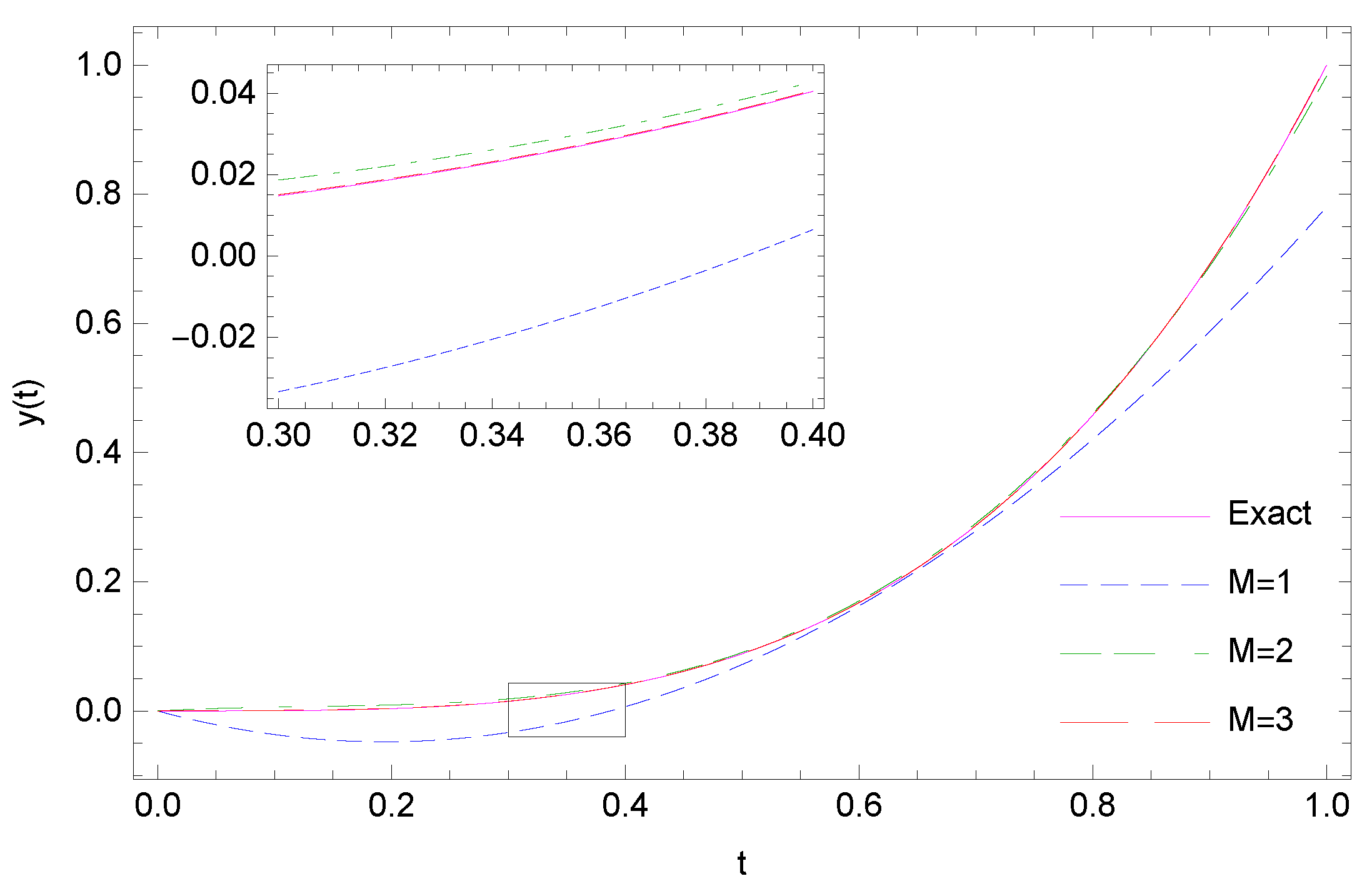
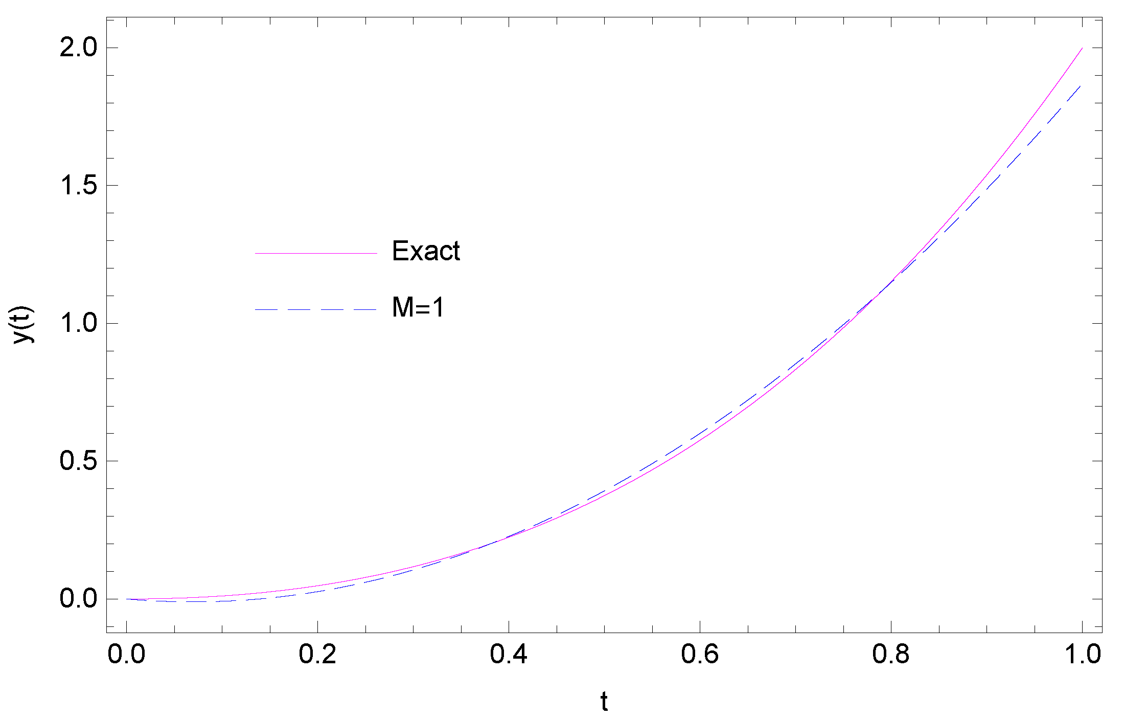
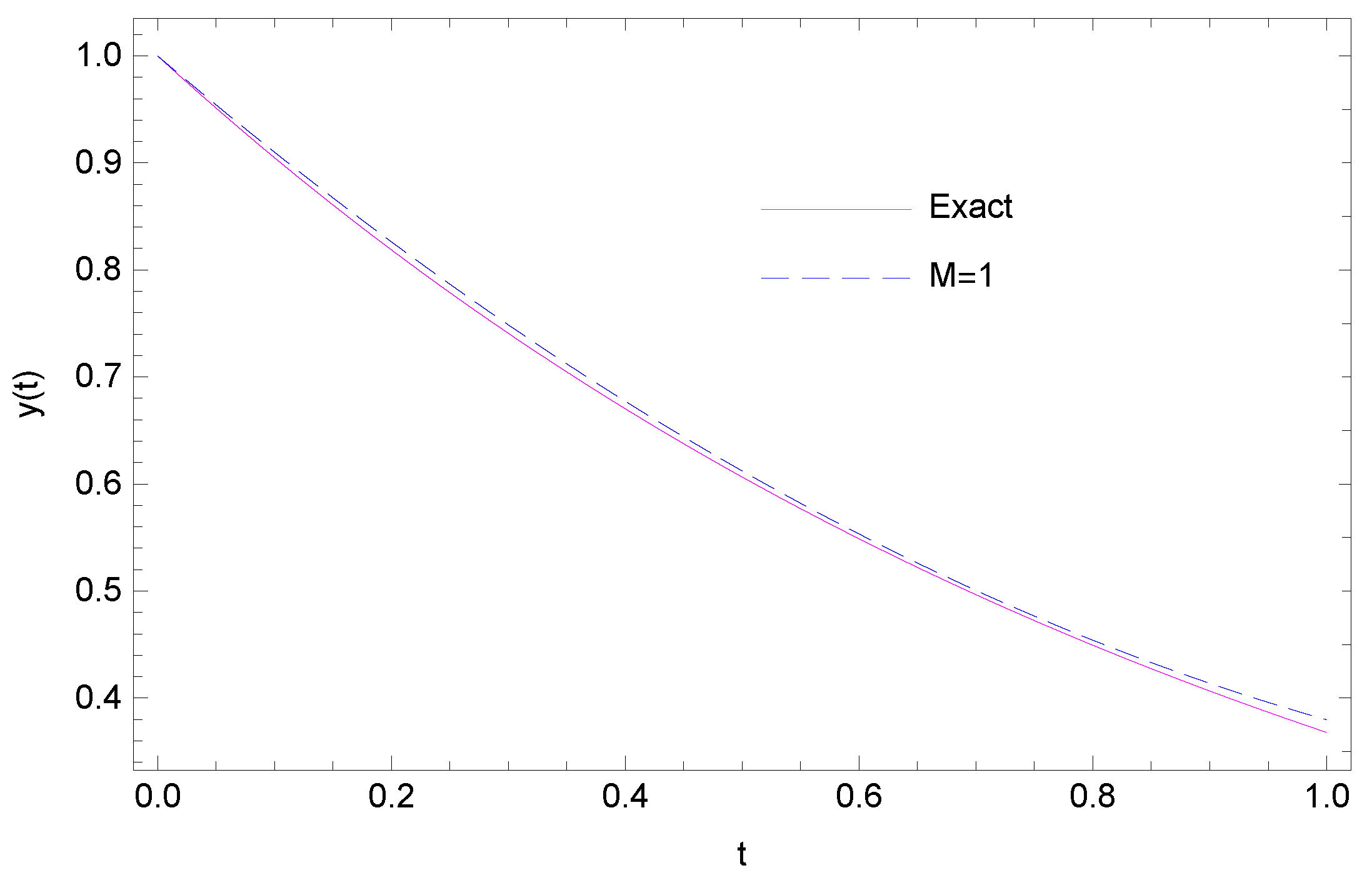
6. Illustrative Examples

In this section, we apply our method to some variable-order FDEs and, moreover, to one variable-order fractional pantograph differential equation (Example 4), comparing the results with the ones obtained by existing methods in the literature. We implemented our method and performed our numerical simulations with Mathematica 12.

Example 1.

In our first example, we considered the following multiterm variable-order FDE [19,22,23]:

$${{}_0^{C}D}_t^{2t}y\left(t\right)+t^{\frac{1}{2}}{{}_0^{C}D}_t^{\frac{t}{3}}y\left(t\right)+t^{\frac{1}{3}}{{}_0^{C}D}_t^{\frac{t}{4}}y\left(t\right)+t^{\frac{1}{4}}{{}_0^{C}D}_t^{\frac{t}{5}}y\left(t\right)+t^{\frac{1}{5}}y\left(t\right)=g\left(t\right),0<t\le 1,$$

(27)

where

$$g\left(t\right)=-\frac{t^{2-2t}}{\Gamma (3-2t)}-t^{\frac{1}{2}}\frac{t^{2-\frac{t}{3}}}{\Gamma (3-\frac{t}{3})}-t^{\frac{1}{3}}\frac{t^{2-\frac{t}{4}}}{\Gamma (3-\frac{t}{4})}-t^{\frac{1}{4}}\frac{t^{2-\frac{t}{5}}}{\Gamma (3-\frac{t}{5})}+t^{\frac{1}{5}}\left(2-\frac{t^2}{2}\right)$$

with initial conditions $y\left(0\right)=2$ and $y^{\prime }\left(0\right)=0$. The exact solution to this problem is $y\left(t\right)=2-\frac{t^2}{2}$. As can be seen, we have $\alpha \left(t\right)=2t$. Therefore, to implement the proposed method, we introduce:

$$n=\underset{0<t\le 1}{max}\left\{\lceil 2t\rceil \right\}=2.$$

We set $M=1$ and suppose

$$y{}^{″}\left(t\right)=A^{T}B\left(t\right),$$

where

$$A={\left[a_0,a_1\right]}^T\mathrm{and}B\left(t\right)={\left[1,t-\frac{1}{2}\right]}^T.$$

The operational matrices of variable-order fractional integration are given as follows:

$$P_t^{2-2t}=\left[\begin{array}{cc}\frac{t^{2-2t}}{\Gamma (3-2t)}& 0\\ \frac{t^{2-2t}}{2\Gamma (4-2t)}-\frac{t^{2-2t}}{2\Gamma (3-2t)}& \frac{t^{2-2t}}{\Gamma (4-2t)}\end{array}\right],P_t^{2-\frac{t}{3}}=\left[\begin{array}{cc}\frac{t^{2-\frac{t}{3}}}{\Gamma \left(3-\frac{t}{3}\right)}& 0\\ \frac{t^{2-\frac{t}{3}}}{2\Gamma \left(4-\frac{t}{3}\right)}-\frac{t^{2-\frac{t}{3}}}{2\Gamma \left(3-\frac{t}{3}\right)}& \frac{t^{2-\frac{t}{3}}}{\Gamma \left(4-\frac{t}{3}\right)}\end{array}\right],$$

$$P_t^{2-\frac{t}{4}}=\left[\begin{array}{cc}\frac{t^{2-\frac{t}{4}}}{\Gamma \left(3-\frac{t}{4}\right)}& 0\\ \frac{t^{2-\frac{t}{4}}}{2\Gamma \left(4-\frac{t}{4}\right)}-\frac{t^{2-\frac{t}{4}}}{2\Gamma \left(3-\frac{t}{4}\right)}& \frac{t^{2-\frac{t}{4}}}{\Gamma \left(4-\frac{t}{4}\right)}\end{array}\right],P_t^{2-\frac{t}{5}}=\left[\begin{array}{cc}\frac{t^{2-\frac{t}{5}}}{\Gamma \left(3-\frac{t}{5}\right)}& 0\\ \frac{t^{2-\frac{t}{5}}}{2\Gamma \left(4-\frac{t}{5}\right)}-\frac{t^{2-\frac{t}{5}}}{2\Gamma \left(3-\frac{t}{5}\right)}& \frac{t^{2-\frac{t}{5}}}{\Gamma \left(4-\frac{t}{5}\right)}\end{array}\right].$$

Furthermore, we have:

$$P_t^2=\left[\begin{array}{cc}\frac{t^2}{2}& 0\\ -\frac{t^2}{6}& \frac{t^2}{6}\end{array}\right].$$

Now, using the initial conditions and the aforementioned operational matrices, we obtain the following approximations for $y\left(t\right)$ and its variable-order derivatives:

$$y\left(t\right)=A^T{P}_t^{2}B\left(t\right)+2,{{}_0^{C}D}_t^{2t}y\left(t\right)=A^T{P}_t^{2-2t}B\left(t\right)+\sum _{i=\lceil 2t\rceil }^1{y}_0^i\frac{t^{i-2t}}{\Gamma (i-2t+1)},$$

$$\begin{array}{c}{{}_0^{C}D}_t^{\frac{t}{3}}y\left(t\right)=A^T{P}_t^{2-\frac{t}{3}}B\left(t\right)+\sum _{i=\lceil \frac{t}{3}\rceil }^1{y}_0^i\frac{t^{i-\frac{t}{3}}}{\Gamma (i-\frac{t}{3}+1)},\\ {{}_0^{C}D}_t^{\frac{t}{4}}y\left(t\right)=A^T{P}_t^{2-\frac{t}{4}}B\left(t\right)+\sum _{i=\lceil \frac{t}{4}\rceil }^1{y}_0^i\frac{t^{i-\frac{t}{4}}}{\Gamma (i-\frac{t}{4}+1)},\\ {{}_0^{C}D}_t^{\frac{t}{5}}y\left(t\right)=A^T{P}_t^{2-\frac{t}{5}}B\left(t\right)+\sum _{i=\lceil \frac{t}{5}\rceil }^1{y}_0^i\frac{t^{i-\frac{t}{5}}}{\Gamma (i-\frac{t}{5}+1)}.\end{array}$$

By substituting these approximations into (27), collocating the resulting equation at $t_0=\frac{1}{3}$, $t_1=\frac{2}{3}$, and finally, solving the obtained system, we obtain:

$$a_0=-1,a_1=0.$$

Therefore, we have:

$$y\left(t\right)=[-10]\left[\begin{array}{cc}\frac{t^2}{2}& 0\\ -\frac{t^2}{6}& \frac{t^2}{6}\end{array}\right]\left[\begin{array}{c}1\\ t-\frac{1}{2}\end{array}\right]+2=2-\frac{t^2}{2},$$

which is the exact solution. In this case, since the exact solution is a second-order polynomial, we can obtain it by applying the numerical method with just two basis functions.

Example 2.

In our second example, we considered the following nonlinear variable-order FDE borrowed from [41]:

$$\begin{array}{cc}\hfill & {{}_0^{C}D}_t^{\alpha \left(t\right)}y\left(t\right)+sin\left(t\right)y^2\left(t\right)=g\left(t\right),0<t\le 1,0<\alpha \left(t\right)\le 1,\hfill \\ \hfill & y\left(0\right)=0,\hfill \end{array}$$

where

$$g\left(t\right)=\frac{\Gamma \left(\frac{9}{2}\right)}{\Gamma \left(\frac{9}{2}-\alpha \left(t\right)\right)}{t}^{\frac{7}{2}-\alpha \left(t\right)}+sin\left(t\right)t^7.$$

The exact solution of this problem is $y\left(t\right)=t^{\frac{7}{2}}$. By considering $\alpha \left(t\right)=1-0.5exp(-t)$, we solved this problem with different values of M. The numerical results are displayed in Figure 1 and

Table 1. (Example 2) Absolute errors at some selected points with different M.

t	$\mathit{M}=2$	$\mathit{M}=6$	$\mathit{M}=10$
$0.2$	$5.69\times {10}^{-3}$	$9.75\times {10}^{-6}$	$8.06\times {10}^{-7}$
$0.4$	$2.34\times {10}^{-3}$	$8.02\times {10}^{-6}$	$6.34\times {10}^{-7}$
$0.6$	$2.78\times {10}^{-3}$	$7.03\times {10}^{-6}$	$5.53\times {10}^{-7}$
$0.8$	$2.52\times {10}^{-3}$	$5.97\times {10}^{-6}$	$4.59\times {10}^{-7}$
$1.0$	$1.66\times {10}^{-2}$	$2.89\times {10}^{-5}$	$1.95\times {10}^{-6}$

. In Figure 1, the approximate solutions obtained with $M=1,2,3$, together with the exact solution of this problem, are plotted. Furthermore, by considering $M=2,6,10$, the absolute errors at some selected points are reported in Table 1. From these results, the convergence of the numerical solutions to the exact one can be easily seen.

Example 3.

Consider the following variable-order FDE taken from [42]:

$$\begin{array}{cc}\hfill & {{}_0^{C}D}_t^{sin\left(t\right)}y\left(t\right)+y\left(t\right)+e^{t}y\left(t^5\right)=g\left(t\right),0<t\le 1,\hfill \\ \hfill & y\left(0\right)=0,\hfill \end{array}$$

(28)

where

$$g\left(t\right)=\frac{\Gamma \left(4\right)}{\Gamma (4-sin(t\left)\right)}{t}^{3-sin\left(t\right)}+\frac{\Gamma \left(3\right)}{\Gamma (3-sin(t\left)\right)}{t}^{2-sin\left(t\right)}+e^t(t^{15}+t^{10})+t^3+t^2.$$

The exact solution of this problem is $y\left(t\right)=t^3+t^2$. To solve Problem (28), we applied the method with $M=1$ and $M=2$. The numerical solution obtained with $M=1$, together with the exact solution are plotted in Figure 2. With $M=2$, according to the method described in Section 4, we set $n={max}_{0<t\le 1}\left\{\lceil sin\left(t\right)\rceil \right\}=1$. Therefore, by assuming that

$$y^{\prime }\left(t\right)=A^{T}B\left(t\right),$$

and using the initial condition, we have:

$$y\left(t\right)=A^T{P}_t^{1}B\left(t\right),{{}_0^{C}D}_t^{sin\left(t\right)}y\left(t\right)=A^T{P}_t^{1-sin\left(t\right)}B\left(t\right),y\left(t^5\right)=A^T{P}_{t^5}^{1}B\left(t^5\right).$$

By substituting these approximations into (28) and using the collocation points $t_0=\frac{1}{4}$, $t_1=\frac{1}{2}$, and $t_2=\frac{3}{4}$, we obtain a system of three nonlinear algebraic equations in terms of the elements of the vector A. By solving the resulting system, one obtains:

$$a_0=2,a_1=5,a_2=3.$$

Finally, using these values, we obtain:

$$y\left(t\right)=\left[\begin{array}{ccc}2& 5& 3\end{array}\right]\left[\begin{array}{ccc}t& 0& 0\\ -\frac{t}{4}& \frac{t}{2}& 0\\ \frac{t}{36}& -\frac{t}{6}& \frac{t}{3}\end{array}\right]\left[\begin{array}{c}1\\ t-\frac{1}{2}\\ t^2-t+\frac{1}{6}\end{array}\right]=t^3+t^2,$$

which is the exact solution.

Example 4.

Let us now consider the fractional pantograph differential equation:

$$\begin{array}{cc}\hfill & {{}_0^{C}D}_t^{\alpha \left(t\right)}y\left(t\right)+y\left(t\right)-0.1y\left(0.2t\right)=-0.1e^{-0.2t},0<t\le 1,0<\alpha \left(t\right)\le 1,\hfill \\ \hfill & y\left(0\right)=1.\hfill \end{array}$$

(29)

The exact solution of this problem, when $\alpha \left(t\right)=1$, is $y\left(t\right)=e^{-t}$. By choosing $M=1$ and $\alpha \left(t\right)=1$, we set:

$$y^{\prime }\left(t\right)=A^{T}B\left(t\right).$$

Then, by considering the initial condition, we have:

$$y\left(t\right)=A^T{P}_t^{1}B\left(t\right)+1,y\left(0.2\right)=A^T{P}_{0.2t}^{1}B\left(0.2t\right)+1.$$

By substituting these approximations into (29), and using the collocation points

$$t_0=\frac{1}{3},t_1=\frac{2}{3},$$

we obtain

$$a_0=-0.620328,a_1=0.621053,$$

which gives

$$y\left(t\right)=\left[\begin{array}{cc}-0.620328& 0.621053\end{array}\right]\left[\begin{array}{cc}t& 0\\ -\frac{t}{4}& \frac{t}{2}\end{array}\right]\left[\begin{array}{c}1\\ t-\frac{1}{2}\end{array}\right]+1=0.310526t^2-0.930854t+1.$$

This approximate solution and the exact solution to the problem, corresponding to $\alpha =1$, are displayed in Figure 3. By computing the $L^2$-norm of the error for this approximation, we have:

$${∥e^{-t}-(0.310526t^2-0.930854t+1)∥}_2=6.29\times {10}^{-3},$$

which shows that the method gives a high-accuracy approximate solution, even with a small number of basis functions. A comparison of the absolute errors, obtained by the proposed method with $M=6,8,10$ at some selected points, with the results proposed in [43], using modified hat functions, and those of [44], using Bernoulli wavelets, are reported in

Table 2. (Example 4) Comparison of absolute errors, at some selected grid points, with $\alpha \left(t\right)=1$.

	Method of [43]	Method of [44]	Present Method
$\mathit{t}$	$\mathit{n}=\mathbf{64}$	$\mathit{k}=\mathbf{2},\mathit{M}=\mathbf{6}$	$\mathit{M}=\mathbf{6}$	$\mathit{M}=\mathit{8}$	$\mathit{M}=\mathbf{10}$
$2^{-2}$	$1.18\times {10}^{-9}$	$1.05\times {10}^{-8}$	$8.61\times {10}^{-9}$	$1.37\times {10}^{-11}$	$5.56\times {10}^{-13}$
$2^{-3}$	$5.39\times {10}^{-10}$	$5.79\times {10}^{-9}$	$1.01\times {10}^{-8}$	$1.57\times {10}^{-11}$	$4.25\times {10}^{-13}$
$2^{-4}$	$1.17\times {10}^{-9}$	$2.00\times {10}^{-8}$	$9.30\times {10}^{-9}$	$1.59\times {10}^{-11}$	$2.42\times {10}^{-13}$
$2^{-5}$	$5.34\times {10}^{-10}$	$3.70\times {10}^{-9}$	$6.47\times {10}^{-9}$	$1.21\times {10}^{-11}$	$1.29\times {10}^{-13}$
$2^{-6}$	$2.27\times {10}^{-9}$	$2.03\times {10}^{-8}$	$3.83\times {10}^{-9}$	$7.58\times {10}^{-12}$	$6.72\times {10}^{-14}$

. From this table, it is seen that our method gave more accurate results with a smaller number of basis functions when compared to previous methods. Moreover, the approximate solutions obtained with $M=2$ and different $\alpha \left(t\right)$, along with the exact solution of corresponding first-order equation, are given in Figure 4. This figure shows that the numerical solution is close to the exact solution for the case $\alpha \left(t\right)=1$ when $\alpha \left(t\right)$ is close to one.

Example 5.

As our last example, consider the following variable-order FDE found in [45]:

$$\begin{array}{c}\hfill {{}_0^{C}D}_t^{\alpha \left(t\right)}y\left(t\right)+3y^{\prime }\left(t\right)-y\left(t\right)=e^t\left(3-\frac{\Gamma (1-\alpha (t),t)}{\Gamma (1-\alpha (t\left)\right)}\right),0<t\le 1,\end{array}$$

where $\alpha \left(t\right)=0.25(1+{cos}^2\left(t\right))$ and the initial condition is $y\left(0\right)=1$. The exact solution is $y\left(t\right)=e^t$. We solved this problem using the proposed method in this paper with different values of M. A comparison of the absolute errors at some selected points, obtained by our method and the one of [45], based on a class of Lagrange polynomials, is given in

Table 3. (Example 5) Comparison of the absolute errors at some selected grid points.

	Method of [45]		Present Method
$\mathit{t}$	$\mathit{M}=\mathbf{6}$	$\mathit{M}=\mathbf{10}$	$\mathit{M}=\mathbf{6}$	$\mathit{M}=\mathbf{8}$	$\mathit{M}=\mathbf{10}$
$0.1$	$8.66\times {10}^{-9}$	$1.04\times {10}^{-12}$	$2.56\times {10}^{-8}$	$4.12\times {10}^{-11}$	$4.40\times {10}^{-14}$
$0.3$	$1.60\times {10}^{-8}$	$4.57\times {10}^{-14}$	$2.43\times {10}^{-8}$	$3.92\times {10}^{-11}$	$4.23\times {10}^{-14}$
$0.5$	$2.49\times {10}^{-8}$	$2.82\times {10}^{-11}$	$2.44\times {10}^{-8}$	$3.93\times {10}^{-11}$	$4.24\times {10}^{-14}$
$0.7$	$4.19\times {10}^{-8}$	$3.12\times {10}^{-11}$	$2.47\times {10}^{-8}$	$3.98\times {10}^{-11}$	$4.29\times {10}^{-14}$
$0.9$	$5.93\times {10}^{-8}$	$1.46\times {10}^{-10}$	$2.56\times {10}^{-8}$	$4.14\times {10}^{-11}$	$4.43\times {10}^{-14}$

.

7. Concluding Remarks

Many researchers have employed fractional differential equations (FDEs) in order to model and analyze various scientific phenomena. Typically, such FDEs do not have known analytical solutions, and approximate and numerical approaches have to be applied [46]. Here, a new numerical method, based on Bernoulli polynomials, was presented for solving multiterm variable-order fractional differential equations. The operational matrix of variable-order fractional integration for the Bernoulli basis functions was introduced, which is a lower triangular matrix and helps to reduce the computational effort of the method. Our scheme uses this matrix to give some approximations of the unknown solution of the problem and its variable-order fractional derivatives in terms of the Bernoulli functions. Substituting these approximations into the equation and using some collocation points allowed us to reduce the problem to a system of nonlinear algebraic equations, which greatly simplifies the problem. An error estimate of the method was proven, and the applicability of our method was illustrated by solving five illustrative examples. The obtained results confirmed the efficiency, accuracy, and high performance of our technique, when compared with the state-of-the-art numerical schemes available in the literature. We emphasize that the accuracy of our method is preserved even when the solution of the problem is not infinitely differentiable. This can be observed in Example 2, whose exact solution is $t^{\frac{7}{2}}$.

We used a variable-order definition where the operator has no order memory, a so-called type-I operator. As future work, it would be interesting to extend the proposed numerical method to approximate variable-order derivatives with weak (type-II) and strong (type-III) variable-order definitions [18,47]. Other interesting lines of research include the stability analysis of the proposed numerical method and its application to different areas in science and engineering, for example in structural mechanics.

References

1. Almeida, R.; Tavares, D.; Torres, D.F.M. The Variable-Order Fractional Calculus of Variations; Springer: Cham, Switzerland, 2019. [Google Scholar] [CrossRef] [Green Version]
2. Samko, S.G.; Kilbas, A.A.; Marichev, O.I. Fractional Integrals and Derivatives; Translated from the 1987 Russian Original; Gordon and Breach: Yverdon, Switzerland, 1993. [Google Scholar]
3. Podlubny, I. Fractional Differential Equations; Academic Press: San Diego, CA, USA, 1999. [Google Scholar]
4. Kilbas, A.A.; Srivastava, H.M.; Trujillo, J.J. Theory and Applications of Fractional Differential Equations; Elsevier: Amsterdam, The Netherlands, 2006. [Google Scholar]
5. Mainardi, F. Fractional Calculus and Waves in Linear Viscoelasticity; Imperial College Press: London, UK, 2010. [Google Scholar] [CrossRef]
6. Tuan, N.H.; Ganji, R.M.; Jafari, H. A numerical study of fractional rheological models and fractional Newell-Whitehead-Segel equation with nonlocal and nonsingular kernel. Chin. J. Phys. 2020, 68, 308–320. [Google Scholar] [CrossRef]
7. Samko, S.G.; Ross, B. Integration and differentiation to a variable fractional order. Integr. Transf. Spec. Funct. 1993, 1, 277–300. [Google Scholar] [CrossRef]
8. Odzijewicz, T.; Malinowska, A.B.; Torres, D.F.M. Noether’s theorem for fractional variational problems of variable order. Cent. Eur. J. Phys. 2013, 11, 691–701. [Google Scholar] [CrossRef] [Green Version]
9. Chen, S.; Liu, F.; Burrage, K. Numerical simulation of a new two-dimensional variable-order fractional percolation equation in non-homogeneous porous media. Comput. Math. Appl. 2014, 67, 1673–1681. [Google Scholar] [CrossRef]
10. Coimbra, C.F.M.; Soon, C.M.; Kobayashi, M.H. The variable viscoelasticity operator. Ann. Phys. 2005, 14, 378–389. [Google Scholar] [CrossRef]
11. Odzijewicz, T.; Malinowska, A.B.; Torres, D.F.M. Fractional Variational Calculus of Variable Order. In Advances in Harmonic Analysis and Operator Theory. Operator Theory: Advances and Applications; Almeida, A., Castro, L., Speck, F.O., Eds.; Birkhäuser: Basel, Switzerland, 2013; Volume 229, pp. 291–301. [Google Scholar] [CrossRef] [Green Version]
12. Ostalczyk, P.W.; Duch, P.; Brzeziński, D.W.; Sankowski, D. Order functions selection in the variable fractional-order PID controller. Advances in Modelling and Control of Non-integer-Order Systems. Lect. Notes Electr. Eng. 2015, 320, 159–170. [Google Scholar] [CrossRef]
13. Rapaić, M.R.; Pisano, A. Variable-order fractional operators for adaptive order and parameter estimation. IEEE Trans. Autom. Contr. 2014, 59, 798–803. [Google Scholar] [CrossRef]
14. Patnaik, S.; Semperlotti, F. Variable-order particle dynamics: Formulation and application to the simulation of edge dislocations. Philos. Trans. R. Soc. A 2020, 378, 20190290. [Google Scholar] [CrossRef]
15. Blaszczyk, T.; Bekus, K.; Szajek, K.; Sumelka, W. Approximation and application of the Riesz-Caputo fractional derivative of variable order with fixed memory. Meccanica 2021, in press. [Google Scholar] [CrossRef]
16. Di Paola, M.; Alotta, G.; Burlon, A.; Failla, G. A novel approach to nonlinear variable-order fractional viscoelasticity. Philos. Trans. R. Soc. A 2020, 378, 20190296. [Google Scholar] [CrossRef]
17. Burlon, A.; Alotta, G.; Di Paola, M.; Failla, G. An original perspective on variable-order fractional operators for viscoelastic materials. Meccanica 2021, 56, 769–784. [Google Scholar] [CrossRef]
18. Patnaik, S.; Jokar, M.; Semperlotti, F. Variable-order approach to nonlocal elasticity: Theoretical formulation, order identification via deep learning, and applications. Comput. Mech. 2021, in press. [Google Scholar] [CrossRef]
19. El-Sayed, A.A.; Agarwal, P. Numerical solution of multiterm variable-order fractional differential equations via shifted Legendre polynomials. Math. Meth. Appl. Sci. 2019, 42, 3978–3991. [Google Scholar] [CrossRef]
20. Wang, L.F.; Ma, Y.P.; Yang, Y.Q. Legendre polynomials method for solving a class of variable order fractional differential equation. CMES-Comp. Model. Eng. 2014, 101, 97–111. [Google Scholar] [CrossRef]
21. Chen, Y.M.; Wei, Y.Q.; Liu, D.Y.; Yu, H. Numerical solution for a class of nonlinear variable order fractional differential equations with Legendre wavelets. Appl. Math. Lett. 2015, 46, 83–88. [Google Scholar] [CrossRef]
22. Liu, J.; Li, X.; Wu, L. An operational matrix of fractional differentiation of the second kind of Chebyshev polynomial for solving multiterm variable order fractional differential equation. Math. Probl. Eng. 2016, 2016, 7126080. [Google Scholar] [CrossRef] [Green Version]
23. Nagy, A.M.; Sweilam, N.H.; El-Sayed, A.A. New operational matrix for solving multiterm variable order fractional differential equations. J. Comput. Nonlinear Dyn. 2018, 13, 11001–11007. [Google Scholar] [CrossRef]
24. Chen, Y.M.; Liu, L.Q.; Li, B.F.; Sun, Y. Numerical solution for the variable order linear cable equation with Bernstein polynomials. Appl. Math. Comput. 2014, 238, 329–341. [Google Scholar] [CrossRef]
25. Tavares, D.; Almeida, R.; Torres, D.F.M. Caputo derivatives of fractional variable order: Numerical approximations. Commun. Nonlinear Sci. 2016, 35, 69–87. [Google Scholar] [CrossRef] [Green Version]
26. Shen, S.; Liu, F.; Chen, J.; Turner, I.; Anh, V. Numerical techniques for the variable order time fractional diffusion equation. Appl. Math. Comput. 2012, 218, 10861–10870. [Google Scholar] [CrossRef] [Green Version]
27. Hammouch, Z.; Yavuz, M.; Özdemir, N. Numerical solutions and synchronization of a variable-order fractional chaotic system. Math. Model. Numer. Simul. Appl. 2021, 1, 11–23. [Google Scholar] [CrossRef]
28. Ganji, R.M.; Jafari, H.; Baleanu, D. A new approach for solving multi variable orders differential equations with Mittag-Leffler kernel. Chaos Solitons Fractals 2020, 130, 109405. [Google Scholar] [CrossRef]
29. Eghbali, A.; Johansson, H.; Saramäki, T. A method for the design of Farrow-structure based variable fractional-delay FIR filters. Signal Process. 2013, 93, 1341–1348. [Google Scholar] [CrossRef]
30. Yu, C.; Teo, K.L.; Dam, H.H. Design of all pass variable fractional delay filter with signed powers-of-two coefficients. Signal Process. 2014, 95, 32–42. [Google Scholar] [CrossRef]
31. Cooper, G.R.J.; Cowan, D.R. Filtering using variable order vertical derivatives. Comput. Geosci. 2004, 30, 455–459. [Google Scholar] [CrossRef]
32. Tseng, C.-C. Design of variable and adaptive fractional order FIR differentiators. Signal Process. 2006, 86, 2554–2566. [Google Scholar] [CrossRef]
33. Bhrawy, A.H.; Tohidi, E.; Soleymani, F. A new Bernoulli matrix method for solving high-order linear and nonlinear Fredholm integro-differential equations with piecewise intervals. Appl. Math. Comput. 2012, 219, 482–497. [Google Scholar] [CrossRef]
34. Tohidi, E.; Bhrawy, A.H.; Erfani, K. A collocation method based on Bernoulli operational matrix for numerical solution of generalized pantograph equation. Appl. Math. Model. 2013, 37, 4283–4294. [Google Scholar] [CrossRef]
35. Toutounian, F.; Tohidi, E. A new Bernoulli matrix method for solving second order linear partial differential equations with the convergence analysis. Appl. Math. Comput. 2013, 223, 298–310. [Google Scholar] [CrossRef]
36. Bazm, S. Bernoulli polynomials for the numerical solution of some classes of linear and nonlinear integral equations. J. Comput. Appl. Math. 2015, 275, 44–60. [Google Scholar] [CrossRef]
37. Keshavarz, E.; Ordokhani, Y.; Razzaghi, M. A numerical solution for fractional optimal control problems via Bernoulli polynomials. J. Vib. Control 2016, 22, 3889–3903. [Google Scholar] [CrossRef]
38. Costabile, F.; Dellaccio, F.; Gualtieri, M.I. A new approach to Bernoulli polynomials. Rend. Mat. Ser. VII 2006, 26, 1–12. [Google Scholar]
39. Arfken, G. Mathematical Methods for Physicists, 3rd ed.; Academic Press: San Diego, CA, USA, 1985. [Google Scholar]
40. Mason, J.C.; Handscomb, D.C. Chebyshev Polynomials; CRC Press LLC: Boca Raton, FL, USA, 2003. [Google Scholar]
41. Hassani, H.; Dahaghin, M.S.; Heydari, H. A new optimized method for solving variable-order fractional differential equations. J. Math. Ext. 2017, 11, 85–98. [Google Scholar]
42. Li, X.; Li, H.; Wu, B. A new numerical method for variable order fractional functional differential equations. Appl. Math. Lett. 2017, 68, 80–86. [Google Scholar] [CrossRef]
43. Nemati, S.; Lima, P.; Sedaghat, S. An effective numerical method for solving fractional pantograph differential equations using modification of hat functions. Appl. Numer. Math. 2018, 131, 174–189. [Google Scholar] [CrossRef]
44. Rahimkhani, P.; Ordokhani, Y.; Babolian, E. A new operational matrix based on Bernoulli wavelets for solving fractional delay differential equations. Numer. Algorithms 2017, 74, 223–245. [Google Scholar] [CrossRef]
45. Sabermahani, S.; Ordokhani, Y.; Lima, P.M. A novel Lagrange operational matrix and Tau-collocation method for solving variable-order fractional differential equations. Iran J. Sci. Technol. Trans. Sci. 2020, 44, 127–135. [Google Scholar] [CrossRef]
46. Nikan, O.; Jafari, H.; Golbabai, A. Numerical analysis of the fractional evolution model for heat flow in materials with memory. Alex. Eng. J. 2020, 59, 2627–2637. [Google Scholar] [CrossRef]
47. Lorenzo, C.F.; Hartley, T.T. Variable order and distributed order fractional operators. Nonlinear Dyn. 2002, 29, 57–98. [Google Scholar] [CrossRef]
Figure 1. (Example 2) Comparison between the exact solution and numerical solutions with M = 1 , 2 , 3 .
Fractalfract 05 00219 g001
Figure 2. (Example 3) Comparison between the exact solution and numerical solution with M = 1 .
Fractalfract 05 00219 g002
Figure 3. (Example 4) Comparison between exact and numerical solutions with M = 1 and α ( t ) = 1 .
Fractalfract 05 00219 g003
Figure 4. (Example 4) Approximate solutions with M = 2 and different α ( t ) , together with the exact solution for α ( t ) = 1 .
Fractalfract 05 00219 g004