Anomalous Stochastic Transport of Particles with Self-Reinforcement and Mittag–Leffler Distributed Rest Times

Abstract

We introduce a persistent random walk model for the stochastic transport of particles involving self-reinforcement and a rest state with Mittag–Leffler distributed residence times. The model involves a system of hyperbolic partial differential equations with a non-local switching term described by the Riemann–Liouville derivative. From Monte Carlo simulations, we found that this model generates superdiffusion at intermediate times but reverts to subdiffusion in the long time asymptotic limit. To confirm this result, we derived the equation for the second moment and find that it is subdiffusive in the long time limit. Analyses of two simpler models are also included, which demonstrate the dominance of the Mittag–Leffler rest state leading to subdiffusion. The observation that transient superdiffusion occurs in an eventually subdiffusive system is a useful feature for applications in stochastic biological transport.

1. Introduction

The stochastic movement of intracellular organelles, cells and animals very often exhibits anomalous diffusion, which has led to the widespread use of fractional diffusion equations and fractional derivatives in modeling [1,2]. There are several recent observations that emphasize the importance of fractional models in biological phenomena, such as cancer cell motility [3], polarized cell dynamics [4], intracellular transport of organelles [5] and animal migration [6]. In particular, we can observe superdiffusive and subdiffusive transport simultaneously in intracellular transport [5,7,8]. Recently, superdiffusion was modeled by a persistent random walk model using the concept of self-reinforcing directionality [9,10]. However, it is well known that endosomes alternate between active movement along microtubules and resting in the cytoplasm, with these rest times being power-law distributed [8,9]. Therefore, it is natural to formulate a self-reinforcing, persistent random walk model with Mittag–Leffler distributed rest times, which have power-law tails.

For continuous time random walks (CTRW), the competition between power-law run and rest times has been explored thoroughly [11,12,13]. Recently, a model based on the elephant random walk [14] with reinforcement exhibiting superdiffusion, diffusion and subdiffusion at the long time limit has been formulated in discrete time and space [15]. The model presented here is actually a generalization of the elephant random walk model [14,16,17,18,19,20,21,22], a jump process, to a persistent random walk framework with finite velocity [2,23,24]. Using the persistent random walk framework is advantageous, as extensions such as reactions, chemosensitive movement and interactions between agents are established in the literature [25,26,27,28,29,30,31,32,33] and convenient to introduce. The purpose of our paper is to explore the impact of an anomalous rest state on self-reinforced persistent random walks with finite velocity.

2. Stochastic Transport with Self-Reinforcement and Mittag–Leffler Distributed Rest Times

To implement rests in a self-reinforcing, persistent random walk model [10], we formulated a model with three states. We introduce the probability density functions (PDFs) for the active states with positive and negative velocity, $p_{+}(x,t)$ and $p_{-}(x,t)$, and the resting state, $p_0(x,t)$. In the active states, the random walk runs with constant speed $\nu$ for an exponentially distributed time with rate $\lambda$. After each active run, the random walk pauses for a Mittag–Leffler distributed residence time and then makes the choice to switch to some next state. With conditional transition probabilities $r_{+}$, $r_{-}$ and $r_0$, the random walk transitions from rest to the positive velocity state, to the negative velocity state, or remains in the rest state ($r_{+}+r_{-}+r_0=1$). An illustration of this is shown in Figure 1. The PDEs that represent this random walk are

$$\begin{array}{cc}\hfill \frac{\partial p_{\pm }}{\partial t}& \pm \nu \frac{\partial p_{\pm }}{\partial x}=-\lambda p_{\pm }+r_{\pm }i(x,t),\hfill \\ \hfill \frac{\partial p_0}{\partial t}& =\lambda p_{+}+\lambda p_{-}-(1-r_0)i(x,t),\hfill \end{array}$$

(1)

where the integral escape rate from the rest state, $i(x,t)$, is defined as follows (see, for example, [34,35,36])

$$i(x,t)={\tau }_0^{-\beta }{\mathcal{D}}_t^{1-\beta }{p}_0(x,t).$$

(2)

Here, the Riemann–Liouville derivative is

$${\mathcal{D}}_t^{1-\beta }{p}_0(x,t)=\frac{1}{\mathsf{\Gamma }\left(\beta \right)}\frac{\partial }{\partial t}{\int }_0^t\frac{p_0(x,t^{\prime })}{{(t-t^{\prime })}^{1-\beta }}d{t}^{\prime }(0<\beta <1).$$

(3)

Note that for the non-Markovian alternating states, one can use the general expression for the escape rate $i(x,t)$ in the form of convolution of the memory kernel and density [37].

In what follows, we will introduce and explain the two key components in the model (1): self-reinforcement and Mittag–Leffler distributed rest times.

Self-reinforcement. Firstly, introducing self-reinforcement to (1) requires careful consideration of the conditional transition probabilities. What really is self-reinforcement, and how does one introduce it in (1)? If a process is self-reinforcing, then it retains a memory of its past decisions and uses this history to affect its current decisions. In other words, the random walk should consider its past decisions to transition into positive and negative velocity states and adjust the conditional transition probabilities ($r_{+}$, $r_{-}$ and $r_0$). Looking at Figure 1, the particle or animal should have $r_{+}$, $r_{-}$ and $r_0$ change with time as more decisions are made.

An intuitive formulation of self-reinforcement is that the time spent traveling with velocity $\pm \nu$ determines the probability that the particle will switch to that state. Mathematically,

$$r_{\pm }=w_1\frac{t_{\pm }}{t}+w_2\frac{t_{\mp }}{t}+w_3\frac{t_0}{t}\mathrm{and}{r}_0=w_3,$$

(4)

where $t_{+}/t$, $t_{-}/t$ and $t_0/t$ are the relative times spent in the positive, negative and zero velocity states, respectively, out of the total time elapsed t. The constant prefactors $w_1$, $w_2$ and $w_3$ are weights on each of those relative times and $w_1+w_2+w_3=1$. We set $w_3=1/3$ so that without self-reinforcement the conditional transition probabilities, $r_{+}$, $r_{-}$ and $r_0$ would be the same. Now using $t=t_{+}+t_{-}+t_0$ and $x=x_0+\nu (t_{+}-t_{-})$ in (4), $r_{\pm }$ can be expressed as

$$r_{\pm }=\frac{1}{3}\pm {\alpha }_0\frac{x-x_0}{2\nu t}({\alpha }_0=w_1-w_2),$$

(5)

where ${\alpha }_0$ is the self-reinforcement parameter. The initial position of the random walk is $x_0$, but for simplicity, we will assume $x_0=0$ from now on. If ${\alpha }_0>0$, then $w_1>w_2$ and the time spent in corresponding states increases the probability of future occupation in that state (in (4) $r_{\pm }$ increases more as $t_{\pm }$ increases since $w_1>w_2$). On the other hand, if ${\alpha }_0<0$, then $w_1<w_2$ and time spent in the corresponding states increases the probability of future avoidance of that state ($r_{\pm }$ increases more as $t_{\mp }$ increases since $w_1<w_2$). Intuitively, reinforcement of past behavior can be represented by $w_1>w_2$ and punishment of past behavior as $w_1<w_2$. Equation (5) is a powerful formulation, since we can express self-reinforcement as an additive term to constant and equal conditional transition probabilities of $1/3$. Moreover, this additive term encapsulates the past history of the random walk by accounting for the ratio of current position x to current time t. The second term on the right-hand side of (5) compares how far the particle has moved away from the initial position given the maximum possible position it could have obtained. It is now clear that the superdiffusion generated by this self-reinforcing mechanism [10] is fundamentally different to those generated by power-law flights in CTRW and Lévy walk formulations. We should point out that self-reinforcing directionality is experimentally observed in intracellular transport of endosomes [9]. A possible biological mechanism underlying this self-reinforcement is given in Section VII of [10]. It would be interesting to extend this model to three dimensions, as was done for the diffusion-advection model for intracellular transport in [38].

Mittag–Leffler distributed rest times. The introduction of the integral escape rate, $i(x,t)$ in (2) involving the Riemann–Liouville fractional derivative, is equivalent to the random walker waiting in the rest state for a random time, which has the probability density

$$\psi \left(\tau \right)=-\frac{d}{d\tau }{E}_{\beta }\left[-{\left(\frac{\tau }{{\tau }_0}\right)}^{\beta }\right]\mathrm{where}0<\beta <1,$$

(6)

and $E_{\beta }(·)$ is the one-parameter Mittag–Leffler function. The waiting times in the rest state will be distributed approximately as ${(\tau /{\tau }_0)}^{-1-\beta }$ for large values of $\tau /{\tau }_0$, resulting in “heavy” or power-law tails. The parameter $\beta$ is the measure of the strength of the resting state. As $\beta$ becomes smaller, the probability of a longer residence time is increased. The parameter ${\tau }_0$ is a time scaling. The advantage of using the Mittag–Leffler distribution is that one can obtain the integral escape rate, $i(x,t)$, with the Riemann–Liouville fractional derivative without passing to the long time limit [35,39]. In the limit for $\beta \to 1$, we recover the Markovian case with exponentially distributed resting times, ${\tau }_0^{-1}{e}^{-t/{\tau }_0}$. This component is significant, as power laws are seen in many empirical observations for stochastic processes which possess complex underlying mechanisms [40]. Pertinent examples of power laws include the waiting times between: stock transactions [41], arrivals of internet viruses [42], sudden decreases in terminal airway resistance for lungs with respiratory problems [43], players joining a game network [44], household residence before moving [45], consecutive emails sent [46], dopamine signaling in Drosophila melanogaster [47], and active–passive state switching in endosome movement [8]. All of these examples demonstrate the importance of power-law waiting times in real phenomena, highlighting the need for a self-reinforcing, persistent random walk model with an agent that takes power-law distributed rests while deciding the choice of the next run.

Now, from (1), we can formulate a single governing equation by introducing the total density function $p=p_{+}+p_{-}+p_0$ and the flux $J=\nu (p_{+}-p_{-})$. Then

$$\begin{array}{cc}\hfill \frac{\partial p}{\partial t}& =-\frac{\partial J}{\partial x},\frac{\partial J}{\partial t}=-{\nu }^2\frac{\partial p}{\partial x}+{\nu }^2\frac{\partial p_0}{\partial x}-\lambda J+{\alpha }_0\frac{x}{t}i(x,t),\hfill \\ \hfill \frac{\partial p_0}{\partial t}& =\lambda p-\lambda p_0-(1-r_0)i(x,t).\hfill \end{array}$$

(7)

We can eliminate the flux J by combining the first two equations in (7) and arrive at the governing equations

$$\begin{array}{cc}\hfill \frac{{\partial }^{2}p}{\partial t^2}& +\lambda \frac{\partial p}{\partial t}={\nu }^2\frac{{\partial }^{2}p}{\partial x^2}-{\nu }^2\frac{{\partial }^2{p}_0}{\partial x^2}-\frac{{\alpha }_0}{t}\frac{\partial }{\partial x}\left[x{\tau }_0^{-\beta }{\mathcal{D}}_t^{1-\beta }{p}_0(x,t)\right],\hfill \\ \hfill \frac{\partial p_0}{\partial t}& =\lambda p-\lambda p_0-(1-r_0){\tau }_0^{-\beta }{\mathcal{D}}_t^{1-\beta }{p}_0(x,t),\hfill \end{array}$$

(8)

where for self-reinforcement, $0<{\alpha }_0<2/3$ and $r_0=1/3$. From these governing equations, it is not immediately clear what the effect of Mittag–Leffler distributed rest times will have when competing with self-reinforcement. To elucidate this relationship, we perform second moment calculations in the next section.

3. Second Moment Calculations

From (8), we obtain the fractional differential equations

$$\begin{array}{cc}\hfill \frac{d^2{\mu }_2}{d{t}^2}& +\lambda \frac{d{\mu }_2}{dt}=2{\nu }^2\left[1-N_0\right]+\frac{2{\alpha }_0}{t}{\tau }_0^{-\beta }{\mathcal{D}}_t^{1-\beta }{\mu }_{20},\hfill \\ \hfill \frac{d{\mu }_{20}}{dt}& =\lambda {\mu }_2-\lambda {\mu }_{20}-(1-r_0){\tau }_0^{-\beta }{\mathcal{D}}_t^{1-\beta }{\mu }_{20},\hfill \end{array}$$

(9)

where ${\mu }_2={\int }_{-\infty }^{\infty }{x}^{2}pdx$, ${\mu }_{20}={\int }_{-\infty }^{\infty }{x}^2{p}_{0}dx$ and $N_0={\int }_{-\infty }^{\infty }{p}_{0}dx$. For $N_0$, we can obtain from (8)

$$\frac{d{N}_0}{dt}=\lambda -\lambda N_0-(1-r_0){\tau }_0^{-\beta }{\mathcal{D}}_t^{\beta }{N}_0.$$

(10)

Equation (10) is a fractional differential equation describing the total probability of finding the random walk in the rest state. To simplify calculations, we take the Laplace transform of (9) and (10) along with the initial conditions $p_{+}(x,0)=\delta \left(x\right)$, $p_{-}(x,0)=0$ and $p_0(x,0)=0$ to obtain

$$\begin{array}{cc}\hfill -(s^2+& \lambda s)\frac{d{\widehat{\mu }}_2}{ds}-(2s+\lambda ){\widehat{\mu }}_2=\frac{2{\nu }^2}{s^2}+2{\nu }^2\frac{d{\widehat{N}}_0}{ds}+2{\alpha }_0{\tau }_0^{-\beta }{s}^{1-\beta }{\widehat{\mu }}_{20},\hfill \\ \hfill s{\widehat{\mu }}_{20}& =\lambda {\widehat{\mu }}_2-\lambda {\widehat{\mu }}_{20}-(1-r_0){\tau }_0^{-\beta }{s}^{1-\beta }{\widehat{\mu }}_{20},\hfill \\ \hfill s{\widehat{N}}_0& =\frac{\lambda }{s}-\lambda {\widehat{N}}_0-(1-r_0){\tau }_0^{-\beta }{s}^{1-\beta }{\widehat{N}}_0.\hfill \end{array}$$

(11)

Rearranging and taking the long time limit, $t\to \infty$ ($s\to 0$), the equations in (11) give

$$\begin{array}{cc}\hfill -\lambda s\frac{d{\widehat{\mu }}_2}{ds}& -\lambda {\widehat{\mu }}_2\approx \frac{2{\nu }^2}{s^2}+2{\nu }^2\frac{d{\widehat{N}}_0}{ds}+2{\alpha }_0{\tau }_0^{-\beta }{s}^{1-\beta }{\widehat{\mu }}_{20},\hfill \\ \hfill {\widehat{\mu }}_{20}\approx {\widehat{\mu }}_2& \left(1-\frac{1-r_0}{\lambda }{\tau }_0^{-\beta }{s}^{1-\beta }\right),{\widehat{N}}_0\approx s^{-1}\left(1-\frac{1-r_0}{\lambda }{\tau }_0^{-\beta }{s}^{1-\beta }\right).\hfill \end{array}$$

(12)

By using (12), we obtain a single equation for the second moment in Laplace space

$$-s\frac{d{\widehat{\mu }}_2}{ds}-{\widehat{\mu }}_2\approx \frac{2{\nu }^2(1-r_0)\beta }{{\lambda }^2}{\tau }_0^{-\beta }{s}^{-1-\beta }.$$

(13)

From (13), we obtain the asymptotic second moment in Laplace space as

$${\widehat{\mu }}_2\left(s\right)\sim \frac{2{\nu }^2(1-r_0)}{{\lambda }^2}{\tau }_0^{-\beta }{s}^{-1-\beta },s\to 0.$$

(14)

Finally, taking the inverse Laplace transform,

$${\mu }_2\left(t\right)\sim \frac{2{\nu }^2(1-r_0)}{{\lambda }^2\mathsf{\Gamma }(1+\beta )}{\left(\frac{t}{{\tau }_0}\right)}^{\beta },t\to \infty .$$

(15)

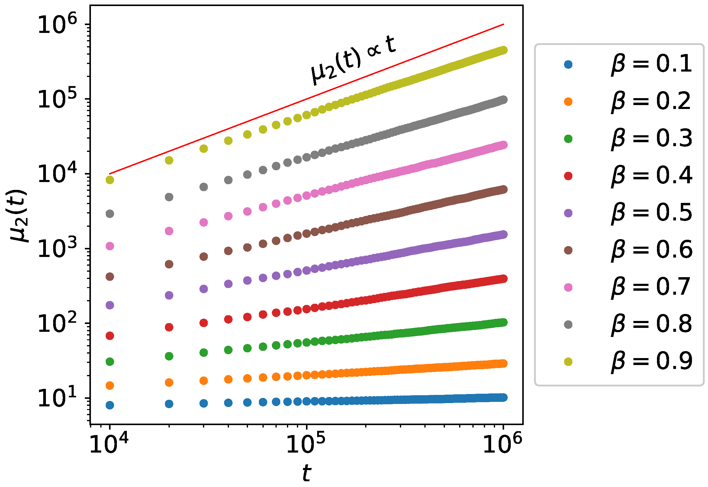
Clearly, (15) demonstrates that the random walk with self-reinforcement (5) and Mittag–Leffler distributed rest times (6) is subdiffusive at the long time limit. This theoretical result is confirmed by the second moment of numerical simulations shown in Figure 2. Interestingly, transient superdiffusion is found in Monte Carlo simulations shown in Figure 3. This suggests that self-reinforcement still plays a major role at shorter time scales but is negated by the eventual trapping of particles in the rest state. This type of behavior is important in intracellular transport, where organelles transition between superdiffusion and subdiffusion at different time scales [8,48].

To understand intuitively what occurs when introducing a heavy-tailed waiting time for the rest state, we consider two simple cases: a single velocity model and a symmetric two velocity model, both with a non-Markovian rest state, and derive their second moments at the long time limit.

3.1. Single Active State Model

As a first example, consider the simplest possible case where there is only one active state with velocity $\nu$ and one rest state, such that the system of fractional differential equations describing this random walk is

$$\begin{array}{cc}\hfill \frac{\partial p_{+}}{\partial t}& +\nu \frac{\partial p_{+}}{\partial x}=-\lambda p_{+}+{\tau }_0^{-\beta }{\mathcal{D}}_t^{1-\beta }{p}_0\hfill \\ \hfill \frac{\partial p_0}{\partial t}& =\lambda p_{+}-{\tau }_0^{-\beta }{\mathcal{D}}_t^{1-\beta }{p}_0.\hfill \end{array}$$

(16)

This simple fractional model can be used to describe the movement of intracellular organelles in only one direction interrupted by rests with Mittag–Leffler distributed residence times.

From (16), we obtain a system of fractional differential equations describing the second moment

$$\frac{d{\mu }_{2+}}{dt}-2\nu {\mu }_{1+}=-\lambda {\mu }_{2+}+{\tau }_0^{-\beta }{\mathcal{D}}_t^{1-\beta }{\mu }_{20},\frac{d{\mu }_{20}}{dt}=\lambda {\mu }_{2+}-{\tau }_0^{-\beta }{\mathcal{D}}_t^{1-\beta }{\mu }_{20},$$

(17)

where ${\mu }_{2+}={\int }_{-\infty }^{\infty }{x}^2{p}_{+}dx$, ${\mu }_{1+}={\int }_{-\infty }^{\infty }x{p}_{+}dx$ and other symbols were defined in (9). By adding together the equations in (17), we find

$$\frac{d{\mu }_2}{dt}=2\nu {\mu }_{1+},$$

(18)

where ${\mu }_2={\mu }_{2+}+{\mu }_{20}$. In order to find ${\mu }_{1+}$, we again use (16) to obtain

$$\frac{d{\mu }_{1+}}{dt}-\nu N_{+}=-\lambda {\mu }_{1+}+{\tau }_0^{-\beta }{\mathcal{D}}_t^{1-\beta }{\mu }_{10},\frac{d{\mu }_{10}}{dt}=\lambda {\mu }_{1+}-{\tau }_0^{-\beta }{\mathcal{D}}_t^{1-\beta }{\mu }_{10},$$

(19)

where $N_{+}={\int }_{-\infty }^{\infty }{p}_{+}dx$ and ${\mu }_{10}={\int }_{-\infty }^{\infty }x{p}_{0}dx$. Recall that our main objective is to find ${\mu }_2$ for which we need ${\mu }_{1+}$, but from (19) it is clear that we also need to find $N_{+}$. Thus, we integrate (16) to obtain

$$\frac{d{N}_{+}}{dt}=-\lambda N_{+}+{\tau }_0^{-\beta }{\mathcal{D}}_t^{1-\beta }{N}_0\left(t\right),\frac{d{N}_0}{dt}=\lambda N_{+}-{\tau }_0^{-\beta }{\mathcal{D}}_t^{1-\beta }{N}_0.$$

(20)

To derive Equations (17), (19) and (20), we have used the fact that $p_{+}(x,t)=p_0(x,t)=0$ and $d{p}_{+}/dx=d{p}_0/dx=0$ as $x\to \pm \infty$. This is because $p_{+}$ and $p_0$ are PDFs that must be normalizable, and additionally, we know that this random walk propagates with finite speed from some initial position.

It is clear that dealing with the Riemann–Liouville derivative in Laplace space will be far easier than attempting to solve (18)–(20) directly. For initial conditions, we assume that the random walk starts in the active state at $x=0$ at $t=0$ such that $p_{+}(x,0)=\delta \left(x\right)$ and $p_0(x,0)=0$. In a similar way to deriving (11), using the initial conditions in conjunction with the Laplace transforms of (18)–(20), we can obtain

$${\widehat{\mu }}_2\left(s\right)\sim \frac{2{\nu }^2}{{\lambda }^2}{\tau }_0^{-2\beta }{s}^{-2\beta -1}.$$

(21)

Finally, taking the inverse Laplace transform,

$${\mu }_2\left(t\right)\sim \frac{2{\nu }^2}{{\lambda }^2\mathsf{\Gamma }(2\beta +1)}{\left(\frac{t}{{\tau }_0}\right)}^{2\beta }.$$

(22)

Using an analogous procedure as above, the first moment for this model can be calculated as ${\mu }_1\left(t\right)\sim \nu t^{\beta }/\lambda {\tau }_0^{\beta }\mathsf{\Gamma }(\beta +1)$. This draws parallels with the fractional Poisson process [49,50,51,52,53,54,55], which has exactly the same time dependence for the first and second moments. In fact, by closely examining (16), we can see the underlying stochastic process for the single active state model is the fractional Poisson process. For (16), the random walk waits in a rest state for a Mittag–Leffler distributed random time and then proceeds to travel with finite velocity $\nu$ for an exponentially distributed random time.

3.2. Bi-Directional Transport Model

The second example we will consider is an extension of the first by adding another active state with velocity $-\nu$. This model is ideal for bi-directional intracellular transport [56] with intermittent resting for power-law distributed times. The system of equations that describes this random walk is

$$\begin{array}{cc}\hfill \frac{\partial p_{\pm }}{\partial t}& \pm \nu \frac{\partial p_{\pm }}{\partial x}=-\lambda p_{\pm }+\frac{1}{2}{\tau }_0^{-\beta }{\mathcal{D}}_t^{1-\beta }{p}_0,\hfill \\ \hfill \frac{\partial p_0}{\partial t}& =\lambda p_{+}+\lambda p_{-}-{\tau }_0^{-\beta }{\mathcal{D}}_t^{1-\beta }{p}_0.\hfill \end{array}$$

(23)

In order to derive an expression for the second moment, we combine the equations in (23), as we did in (1) to obtain (7). Doing this, we find

$$\begin{array}{cc}\hfill \frac{\partial p}{\partial t}& +\frac{\partial J}{\partial x}=0,\frac{\partial J}{\partial t}+{\nu }^2\frac{\partial p}{\partial x}-{\nu }^2\frac{\partial p_0}{\partial x}=-\lambda J,\hfill \\ \hfill \frac{\partial p_0}{\partial t}& =\lambda p-\lambda p_0-{\tau }_0^{-\beta }{\mathcal{D}}_t^{1-\beta }{p}_0.\hfill \end{array}$$

(24)

Again, we can eliminate J by combining the first two equations in (24) to arrive at the governing equations

$$\begin{array}{cc}\hfill \frac{{\partial }^{2}p}{\partial t^2}& +\lambda \frac{\partial p}{\partial t}={\nu }^2\frac{{\partial }^{2}p}{\partial x^2}-{\nu }^2\frac{{\partial }^2{p}_0}{\partial x^2},\hfill \\ \hfill \frac{\partial p_0}{\partial t}& =\lambda p-\lambda p_0-{\tau }_0^{-\beta }{\mathcal{D}}_t^{1-\beta }{p}_0.\hfill \end{array}$$

(25)

We can obtain similar equations to (9) and (10) using (25)

$$\begin{array}{cc}\hfill \frac{d^2{\mu }_2}{d{t}^2}& +\lambda \frac{d{\mu }_2}{dt}=2{\nu }^2-2{\nu }^2{N}_0,\frac{d{\mu }_{20}}{dt}=\lambda {\mu }_2-\lambda {\mu }_{20}-{\tau }_0^{-\beta }{\mathcal{D}}_t^{1-\beta }{\mu }_{20},\hfill \\ \hfill \frac{d{N}_0}{dt}& =\lambda -\lambda N_0-{\tau }_0^{-\beta }{\mathcal{D}}_t^{1-\beta }{N}_0.\hfill \end{array}$$

(26)

Similarly to the first example, using the initial conditions $p_{+}(x,0)=\delta \left(x\right)/2$, $p_{-}(x,0)=\delta \left(x\right)/2$ and $p_0(x,0)=0$, and taking the asymptotic limit as $s\to 0$, we obtain

$${\widehat{N}}_0\left(s\right)\approx \frac{\lambda }{s}\frac{1}{\lambda +{\tau }_0^{-\beta }{s}^{1-\beta }},{\widehat{\mu }}_2\left(s\right)\approx \frac{2{\nu }^2}{\lambda s}\left[\frac{1}{s}-{\widehat{N}}_0\left(s\right)\right].$$

(27)

After substitution, we can find the second moment for the second example at the long time limit as

$${\widehat{\mu }}_2\left(s\right)\sim \frac{2{\nu }^2}{{\lambda }^2}{\tau }_0^{-\beta }{s}^{-1-\beta }.$$

(28)

Finally, taking the inverse Laplace transform,

$${\mu }_2\left(t\right)\sim \frac{2{\nu }^2}{{\lambda }^2\mathsf{\Gamma }(\beta +1)}{\left(\frac{t}{{\tau }_0}\right)}^{\beta },$$

(29)

where $0<\beta <1$. Again, we find that the power-law rests dominate for long times and generate subdiffusion.

For symmetric active states with velocities $\pm \nu$, we found that the second moment is purely subdiffusive, unlike in the first example. In the first example, there was no fractional diffusion limit that could be taken. However, in this second example, the fractional diffusion limit exists, which means that the bi-directional velocity random walk model with Mittag–Leffler distributed rests, (25), can be approximated accurately by the fractional diffusion equation in the long time limit

$$\frac{\partial p}{\partial t}=D_{\beta }\frac{{\partial }^2}{\partial x^2}{\mathcal{D}}_t^{1-\beta }p,$$

(30)

where the fractional diffusion coefficient has an explicit form

$$D_{\beta }=\frac{{\nu }^2}{{\lambda }^2{\tau }_0^{\beta }}.$$

(31)

In order to show that the system (25) at the long time limit leads to the fractional diffusion (30), let us perform the Fourier–Laplace transform of (25). We obtain

$$\widehat{\tilde{p}}(k,s)=\frac{\tilde{p}(k,0)(s+\lambda )}{s^2+s\lambda +{\nu }^2{k}^2-\frac{{\nu }^2\lambda k^2}{s+\lambda +{\tau }_0^{-\beta }{s}^{1-\beta }}}$$

(32)

and at the limit as $s\to 0$,

$$\widehat{\tilde{p}}(k,s)\approx \frac{\tilde{p}(k,0)}{s+D_{\beta }{k}^2{s}^{1-\beta }},$$

(33)

which is exactly the Fourier–Laplace transform of (30). Here we have used ${\partial p/\partial t|}_{t=0}=0$. Note that this well known limit can be obtained from the continuous time random walk model by taking not only the long time limit, but also the large-scale limit [1,2]. Therefore, in the second example, we see that the introduction of a non-Markovian rest state with divergent mean residence time causes the second moment to be subdiffusive. Note that the fractional Equation (16) cannot be approximated by the fractional equation in the same way as (30).

Comparing (15) with (29), we see that the only difference is the constant multiplier $1-r_0$. The non-Markovian rest state (or equivalently, the Mittag–Leffler distributed waiting times for rests) completely neutralizes the superdiffusion generated by the self-reinforcement in the long time limit. Figure 2 demonstrates this by calculating the second moment from simulated trajectories of the random walk corresponding to the system of PDEs in (8).

4. Monte Carlo Simulations

We performed Monte Carlo simulations of the random walk corresponding to (1) to demonstrate that the second moment exhibits subdiffusion. The procedure for such simulations is:

• Initialize variables for current time $T_c=0$, particle position $X_c=0$ and state $S_c=1$. The possible values for $S_c$ are 0, 1 and $-1$ corresponding to the rest, positive velocity and negative velocity states, respectively. For convenience, assume the random walk starts with $S_c=1$.
• Set the constants: $\lambda$, $\beta$, ${\tau }_0$, $\nu$, ${\alpha }_0$, $r_0$ and $t_{end}$, the end time of the simulation.
• If $S_c=0$, generate a random number $\mathsf{\Delta }T=-\lambda ln\left(U\right){[sin\left(\pi \beta \right)/tan\left(\pi \beta V\right)-cos\left(\pi \beta \right)]}^{1/\beta }$, where $U,V\in [0,1)$ are uniformly distributed random numbers (see Equation (20) in [57]). Otherwise, generate a random number $\mathsf{\Delta }T=-ln\left(U\right)/\lambda$.
• Increment simulation time $T_c=T_c+\mathsf{\Delta }T$ and particle position $X_c=X_c+\nu S_c\mathsf{\Delta }T$.
• If $S_c=\pm 1$, then set $S_c=0$. Otherwise, do the following:

  -

  if $0\le W<R_{+}$, set $S_c=1$;

  -

  if $R_{+}\le W<R_{+}+R_{-}$, set $S_c=-1$;

  -

  otherwise, set $S_c=0$;

  where $W\in [0,1)$ is a uniformly distributed random number and $R_{\pm }=r_0\pm {\alpha }_0{X}_c/\left(2\nu T_c\right)$.
• Iterate steps 3 to 5 until $T_c\ge t_{end}$.

All simulations were performed using Python3. To reduce execution time, the “Numba” package and the “multiprocessing” package were used for JIT compilation and CPU parallelization, respectively. We note that if $S_c=0$ initially, then we obtain the same anomalous exponent for ${\mu }_2\left(t\right)$.

Figure 2 confirms the analytical result in (15), which predicted subdiffusion for the long time limit regardless of the strength of self-reinforcement, in this case ${\alpha }_0=0.6$. Interestingly, Figure 3 shows that if ${\tau }_0$ is small, then superdiffusion is possible for intermediate times. As $\beta$ decreases, both Figure 2 and Figure 3 show that subdiffusion increasingly dominates. This was expected, as a smaller value of $\beta$ means stronger trapping in the rest state because of the power-law tails of the Mittag–Leffler distribution.

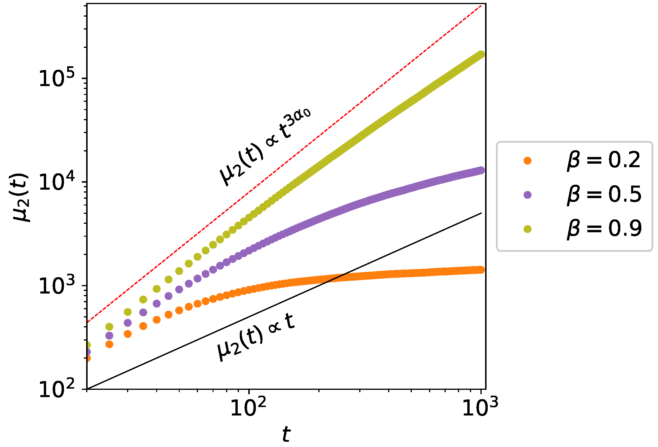
Figure 4 shows that for $\beta =0.9$ the random walk exhibits superdiffusion. However, as time increases, subdiffusion begins to dominate, and is already dominant for $\beta =0.5$ and $0.2$ in Figure 4. We can interpret this transient superdiffusion as a result of competition between the active states with switching rates $\lambda$ and the rest state with anomalous exponent $\beta$ and time scale ${\tau }_0$.

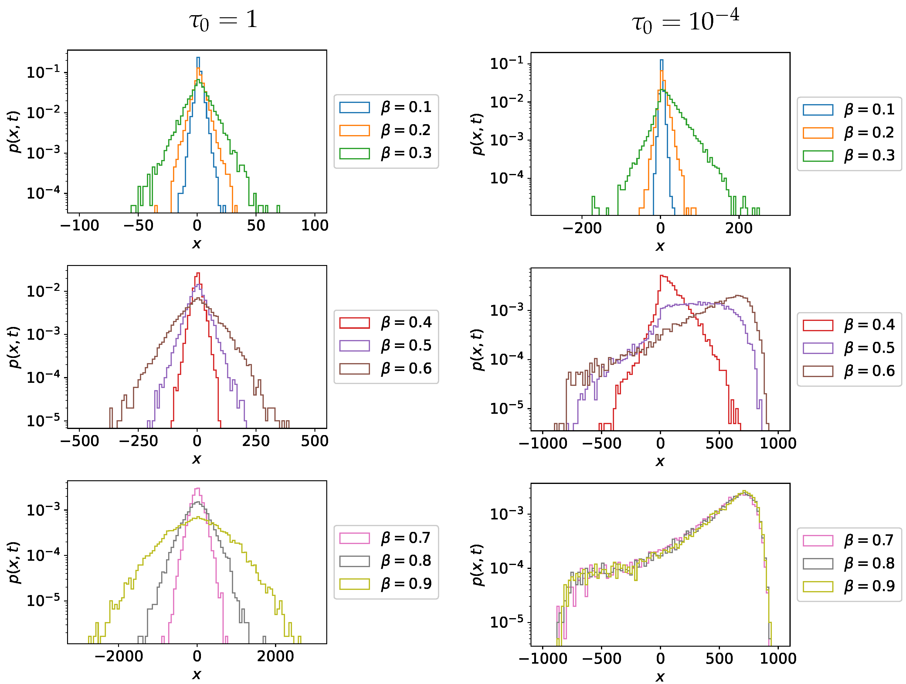
This is further demonstrated by the PDFs observed in Figure 5. Clearly for small values of ${\tau }_0$, the advection caused by self-reinforcement is dominant, leading to a skewed PDF for positive velocity. However for larger ${\tau }_0$, the PDF reverts back to the general shape of Fox functions [1], as expected for subdiffusive random walks. This finding is intriguing, as self-reinforcement places a greater weight on the role of the “characteristic” scale ${\tau }_0$ for the power-law distributed resting times. The fact that transient superdiffusion can occur, for intermediate times in the presence of heavy-tailed resting times, is suggestive of the power of this model to describe natural phenomena with crossover between two exponents of the MSD. Although we obtained subdiffusion at the long time limit, we should emphasize that subdiffusion takes place within a limited time window. Crossover from anomalous to normal diffusion can occur due to truncation or tempering of power-law distributions [58]. Another reason is the thermodynamic uncertainty relation that defines constraints on the time window for anomalous transport [59].

5. Conclusions and Summary

In this paper, we formulated a persistent random walk model for the stochastic transport of particles with self-reinforced directionality and a non-Markovian rest state with Mittag–Leffler distributed residence times. To achieve this, we derived a system of hyperbolic PDEs with a non-local switching term involving the Riemann–Liouville fractional derivative. To investigate the nature of this random walk model, we derived a fractional differential equation for the second moment. We demonstrated analytically and numerically that the introduction of anomalous rests ensures subdiffusion at the long time limit. However, transient superdiffusion was observed for intermediate times, which is also a feature in the intracellular transport of organelles. We further corroborated these results by showing the PDFs of the random walk positions, which exhibit Laplacian distributions at the long time limit but skewed bimodal distributions for intermediate times.

References

1. Metzler, R.; Klafter, J. The random walk’s guide to anomalous diffusion: A fractional dynamics approach. Phys. Rep. 2000, 339, 1–77. [Google Scholar] [CrossRef]
2. Méndez, V.; Fedotov, S.; Horsthemke, W. Reaction-Transport Systems: Mesoscopic Foundations, Fronts, and Spatial Instabilities; Springer Science & Business Media: Berlin, Germany, 2010. [Google Scholar]
3. Huda, S.; Weigelin, B.; Wolf, K.; Tretiakov, K.V.; Polev, K.; Wilk, G.; Iwasa, M.; Emami, F.S.; Narojczyk, J.W.; Banaszak, M.; et al. Lévy-like movement patterns of metastatic cancer cells revealed in microfabricated systems and implicated in vivo. Nat. Commun. 2018, 9, 1–11. [Google Scholar] [CrossRef] [Green Version]
4. Estrada-Rodriguez, G.; Perthame, B. Motility switching and front-back synchronisation in polarized cells. arXiv 2021, arXiv:2109.08981. [Google Scholar]
5. Fedotov, S.; Korabel, N.; Waigh, T.A.; Han, D.; Allan, V.J. Memory effects and Lévy walk dynamics in intracellular transport of cargoes. Phys. Rev. E 2018, 98, 042136. [Google Scholar] [CrossRef] [Green Version]
6. Reynolds, A.M. Current status and future directions of Lévy walk research. Biol. Open 2018, 7, bio030106. [Google Scholar] [CrossRef] [PubMed] [Green Version]
7. Kenwright, D.A.; Harrison, A.W.; Waigh, T.A.; Woodman, P.G.; Allan, V.J. First-passage-probability analysis of active transport in live cells. Phys. Rev. E 2012, 86, 031910. [Google Scholar] [CrossRef]
8. Han, D.; Korabel, N.; Chen, R.; Johnston, M.; Gavrilova, A.; Allan, V.J.; Fedotov, S.; Waigh, T.A. Deciphering anomalous heterogeneous intracellular transport with neural networks. eLife 2020, 9, e52224. [Google Scholar] [CrossRef]
9. Chen, K.; Wang, B.; Granick, S. Memoryless self-reinforcing directionality in endosomal active transport within living cells. Nat. Mater. 2015, 14, 589. [Google Scholar] [CrossRef]
10. Han, D.; da Silva, M.A.; Korabel, N.; Fedotov, S. Self-reinforcing directionality generates truncated Lévy walks without the power-law assumption. Phys. Rev. E 2021, 103, 022132. [Google Scholar] [CrossRef]
11. Portillo, I.G.; Campos, D.; Méndez, V. Intermittent random walks: Transport regimes and implications on search strategies. J. Stat. Mech. Theory Exp. 2011, 2011, P02033. [Google Scholar] [CrossRef]
12. Zaburdaev, V.; Denisov, S.; Klafter, J. Lévy walks. Rev. Mod. Phys. 2015, 87, 483. [Google Scholar] [CrossRef] [Green Version]
13. Klafter, J.; Sokolov, I.M. First Steps in Random Walks: From Tools to Applications; Oxford University Press: Oxford, UK, 2011. [Google Scholar]
14. Schütz, G.M.; Trimper, S. Elephants can always remember: Exact long-range memory effects in a non-Markovian random walk. Phys. Rev. E 2004, 70, 045101. [Google Scholar] [CrossRef] [PubMed] [Green Version]
15. Kumar, N.; Harbola, U.; Lindenberg, K. Memory-induced anomalous dynamics: Emergence of diffusion, subdiffusion, and superdiffusion from a single random walk model. Phys. Rev. E 2010, 82, 021101. [Google Scholar] [CrossRef] [Green Version]
16. Paraan, F.N.C.; Esguerra, J.P. Exact moments in a continuous time random walk with complete memory of its history. Phys. Rev. E 2006, 74, 032101. [Google Scholar] [CrossRef] [Green Version]
17. da Silva, M.; Viswanathan, G.; Cressoni, J. Ultraslow diffusion in an exactly solvable non-Markovian random walk. Phys. Rev. E 2014, 89, 052110. [Google Scholar] [CrossRef] [Green Version]
18. Boyer, D.; Romo-Cruz, J. Solvable random—Walk model with memory and its relations with Markovian models of anomalous diffusion. Phys. Rev. E 2014, 90, 042136. [Google Scholar] [CrossRef] [PubMed] [Green Version]
19. Baur, E.; Bertoin, J. Elephant random walks and their connection to Pólya-type urns. Phys. Rev. E 2016, 94, 052134. [Google Scholar] [CrossRef] [Green Version]
20. Bercu, B.; Chabanol, M.L.; Ruch, J.J. Hypergeometric identities arising from the elephant random walk. J. Math. Anal. Appl. 2019, 480, 123360. [Google Scholar] [CrossRef] [Green Version]
21. Bercu, B.; Laulin, L. On the multi-dimensional elephant random walk. J. Stat. Phys. 2019, 175, 1146–1163. [Google Scholar] [CrossRef] [Green Version]
22. da Silva, M.; Rocha, E.; Cressoni, J.; da Silva, L.; Viswanathan, G. Non-Lévy stable random walk propagators for a non-Markovian walk with both superdiffusive and subdiffusive regimes. Phys. A Stat. Mech. Its Appl. 2020, 538, 122793. [Google Scholar] [CrossRef]
23. Goldstein, S. On diffusion by discontinuous movements, and on the telegraph equation. Q. J. Mech. Appl. Math. 1951, 4, 129–156. [Google Scholar] [CrossRef]
24. Rossetto, V. The one-dimensional asymmetric persistent random walk. J. Stat. Mech. Theory Exp. 2018, 2018, 043204. [Google Scholar] [CrossRef] [Green Version]
25. Othmer, H.G.; Dunbar, S.R.; Alt, W. Models of dispersal in biological systems. J. Math. Biol. 1988, 26, 263–298. [Google Scholar] [CrossRef] [PubMed]
26. Hillen, T. Hyperbolic models for chemosensitive movement. Math. Model. Methods Appl. Sci. 2002, 12, 1007–1034. [Google Scholar] [CrossRef]
27. Fort, J.; Méndez, V. Wavefronts in time-delayed reaction-diffusion systems. Theory and comparison to experiment. Rep. Prog. Phys. 2002, 65, 895. [Google Scholar] [CrossRef]
28. Filbet, F.; Laurençot, P.; Perthame, B. Derivation of hyperbolic models for chemosensitive movement. J. Math. Biol. 2005, 50, 189–207. [Google Scholar] [CrossRef] [PubMed] [Green Version]
29. Fetecau, R.C.; Eftimie, R. An investigation of a nonlocal hyperbolic model for self-organization of biological groups. J. Math. Biol. 2010, 61, 545–579. [Google Scholar] [CrossRef]
30. Bouin, E.; Calvez, V.; Nadin, G. Hyperbolic traveling waves driven by growth. Math. Model. Methods Appl. Sci. 2014, 24, 1165–1195. [Google Scholar] [CrossRef] [Green Version]
31. Perthame, B.; Tang, M.; Vauchelet, N. Derivation of the bacterial run-and-tumble kinetic equation from a model with biochemical pathway. J. Math. Biol. 2016, 73, 1161–1178. [Google Scholar] [CrossRef] [PubMed] [Green Version]
32. Calvez, V. Chemotactic waves of bacteria at the mesoscale. J. Eur. Math. Soc. 2019, 22, 593–668. [Google Scholar] [CrossRef] [Green Version]
33. Kumar, P.; Li, J.; Surulescu, C. Multiscale modeling of glioma pseudopalisades: Contributions from the tumor microenvironment. J. Math. Biol. 2021, 82, 1–45. [Google Scholar] [CrossRef]
34. Angstmann, C.N.; Donnelly, I.C.; Henry, B.I. Continuous time random walks with reactions forcing and trapping. Math. Model. Nat. Phenom. 2013, 8, 17–27. [Google Scholar] [CrossRef] [Green Version]
35. Fedotov, S. Nonlinear subdiffusive fractional equations and the aggregation phenomenon. Phys. Rev. E 2013, 88, 032104. [Google Scholar] [CrossRef] [Green Version]
36. Angstmann, C.N.; Erickson, A.M.; Henry, B.I.; McGann, A.V.; Murray, J.M.; Nichols, J.A. A General Framework for Fractional Order Compartment Models. SIAM Rev. 2021, 63, 375–392. [Google Scholar] [CrossRef]
37. Fedotov, S.; Iomin, A.; Ryashko, L. Non-Markovian models for migration-proliferation dichotomy of cancer cells: Anomalous switching and spreading rate. Phys. Rev. E 2011, 84, 061131. [Google Scholar] [CrossRef] [Green Version]
38. Lin, C.; Ashwin, P.; Steinberg, G. Modelling the motion of organelles in an elongated cell via the coordination of heterogeneous drift–diffusion and long-range transport. Eur. Phys. J. E 2021, 44, 1–15. [Google Scholar] [CrossRef]
39. Mainardi, F.; Raberto, M.; Gorenflo, R.; Scalas, E. Fractional calculus and continuous-time finance II: The waiting-time distribution. Phys. A Stat. Mech. Its Appl. 2000, 287, 468–481. [Google Scholar] [CrossRef] [Green Version]
40. Clauset, A.; Shalizi, C.R.; Newman, M.E. Power-law distributions in empirical data. SIAM Rev. 2009, 51, 661–703. [Google Scholar] [CrossRef] [Green Version]
41. Sabatelli, L.; Keating, S.; Dudley, J.; Richmond, P. Waiting time distributions in financial markets. Eur. Phys. J. B-Condens. Matter Complex Syst. 2002, 27, 273–275. [Google Scholar] [CrossRef]
42. Liebovitch, L.S.; Schwartz, I.B. Information flow dynamics and timing patterns in the arrival of email viruses. Phys. Rev. E 2003, 68, 017101. [Google Scholar] [CrossRef] [Green Version]
43. Suki, B.; Barabási, A.L.; Hantos, Z.; Peták, F.; Stanley, H.E. Avalanches and power-law behaviour in lung inflation. Nature 1994, 368, 615–618. [Google Scholar] [CrossRef]
44. Henderson, T.; Bhatti, S. Modelling user behaviour in networked games. In Proceedings of the Ninth ACM international Conference on Multimedia, Ottawa, ON, Canada, 30 September–5 October 2001; pp. 212–220. [Google Scholar]
45. Fedotov, S.; Stage, H. Anomalous metapopulation dynamics on scale-free networks. Phys. Rev. Lett. 2017, 118, 098301. [Google Scholar] [CrossRef] [PubMed] [Green Version]
46. Barabasi, A.L. The origin of bursts and heavy tails in human dynamics. Nature 2005, 435, 207–211. [Google Scholar] [CrossRef] [Green Version]
47. Ueno, T.; Masuda, N.; Kume, S.; Kume, K. Dopamine modulates the rest period length without perturbation of its power law distribution in Drosophila melanogaster. PLoS ONE 2012, 7, e32007. [Google Scholar] [CrossRef] [PubMed] [Green Version]
48. Korabel, N.; Waigh, T.A.; Fedotov, S.; Allan, V.J. Non-Markovian intracellular transport with sub-diffusion and run-length dependent detachment rate. PLoS ONE 2018, 13, e0207436. [Google Scholar] [CrossRef] [Green Version]
49. Laskin, N. Fractional poisson process. Commun. Nonlinear Sci. Numer. Simul. 2003, 8, 201–213. [Google Scholar] [CrossRef]
50. Mainardi, F.; Gorenflo, R.; Scalas, E. A fractional generalization of the Poisson processes. arXiv 2007, arXiv:math/0701454. [Google Scholar]
51. Mainardi, F.; Gorenflo, R.; Vivoli, A. Beyond the Poisson renewal process: A tutorial survey. J. Comput. Appl. Math. 2007, 205, 725–735. [Google Scholar] [CrossRef] [Green Version]
52. Beghin, L.; Orsingher, E. Poisson-type processes governed by fractional and higher-order recursive differential equations. Electron. J. Probab. 2010, 15, 684–709. [Google Scholar] [CrossRef]
53. Cahoy, D.O.; Uchaikin, V.V.; Woyczynski, W.A. Parameter estimation for fractional Poisson processes. J. Stat. Plan. Inference 2010, 140, 3106–3120. [Google Scholar] [CrossRef] [Green Version]
54. Meerschaert, M.; Nane, E.; Vellaisamy, P. The fractional Poisson process and the inverse stable subordinator. Electron. J. Probab. 2011, 16, 1600–1620. [Google Scholar] [CrossRef]
55. Politi, M.; Kaizoji, T.; Scalas, E. Full characterization of the fractional Poisson process. EPL (Europhys. Lett.) 2011, 96, 20004. [Google Scholar] [CrossRef] [Green Version]
56. Smith, D.A.; Simmons, R.M. Models of motor-assisted transport of intracellular particles. Biophys. J. 2001, 80, 45–68. [Google Scholar] [CrossRef] [Green Version]
57. Fulger, D.; Scalas, E.; Germano, G. Monte Carlo simulation of uncoupled continuous-time random walks yielding a stochastic solution of the space-time fractional diffusion equation. Phys. Rev. E 2008, 77, 021122. [Google Scholar] [CrossRef] [PubMed] [Green Version]
58. Molina-Garcia, D.; Sandev, T.; Safdari, H.; Pagnini, G.; Chechkin, A.; Metzler, R. Crossover from anomalous to normal diffusion: Truncated power-law noise correlations and applications to dynamics in lipid bilayers. New J. Phys. 2018, 20, 103027. [Google Scholar] [CrossRef] [Green Version]
59. Hartich, D.; Godec, A. Thermodynamic Uncertainty Relation Bounds the Extent of Anomalous Diffusion. Phys. Rev. Lett. 2021, 127, 080601. [Google Scholar] [CrossRef] [PubMed]
Figure 1. A diagram that shows a dog and a monotrichous bacterium making the decisions to transition from the rest state to the positive velocity, rest and negative velocity states with the associated conditional transition probabilities, r + , r and r 0 . If the conditional transition probabilities depend on the previous history of choices, r + , r and r 0 should depend on the current position and age.
Fractalfract 05 00221 g001
Figure 2. Plots of second moments for Monte Carlo simulated trajectories. Each value of β has N = 10 4 trajectories. The parameters used were α 0 = 0.6 , ν = 1 , λ = 1 and τ 0 = 1 .
Fractalfract 05 00221 g002
Figure 3. Plots of second moments for Monte Carlo simulated trajectories. Each value of β has N = 10 4 trajectories. The parameters used were α 0 = 0.6 , ν = 1 , λ = 1 and τ 0 = 10 4 .
Fractalfract 05 00221 g003
Figure 4. Plots of second moments for Monte Carlo simulated trajectories. Each value of β has N = 10 4 trajectories. The parameters used were α 0 = 0.6 , ν = 1 , λ = 0.1 and τ 0 = 1 . For clarity, we added the black solid line which corresponds to the second moment of normal diffusion.
Fractalfract 05 00221 g004
Figure 5. Plot of PDFs for Monte Carlo simulated trajectories at t = 10 6 (left column) and t = 10 3 (right column). Each value of β has N = 10 4 trajectories. The parameters used were α 0 = 0.6 , ν = 1 , λ = 1 and τ 0 = 1 (left column) or τ 0 = 10 4 (right column).
Fractalfract 05 00221 g005
Publisher’s Note: MDPI stays neutral with regard to jurisdictional claims in published maps and institutional affiliations.