Phenomenon of Scattering of Zeros of the (p,q)-Cosine Sigmoid Polynomials and (p,q)-Sine Sigmoid Polynomials

Abstract

In this paper, we define $(p,q)$-cosine and sine sigmoid polynomials. Based on this, the properties of each polynomial, and the structure and assumptions of its roots, can be identified. Properties can also be determined by the changes in p and q.

1. Introduction

In [1], R. Chakrabarti and R. Jagannathan first defined the $(p,q)$-number in order to unify varied forms of q-oscillator algebras in the physics literature. Based on this number, mathematicians studied basic and applied theories needed for the mathematics and physics literature; see [2,3,4,5,6,7,8,9].

For any natural number n, the $(p,q)$-number is defined by

$${\left[n\right]}_{p,q}=\frac{p^n-q^n}{p-q},p\ne q.$$

(1)

Based on (1), the theoretical content needed in this paper is summarized as follows.

Definition 1.

Let z be any complex numbers with $\left|z\right|<1$. The two forms of $(p,q)$-exponential functions are defined by

$$e_{p,q}\left(z\right)={\displaystyle \sum _{n=0}^{\infty }}{p}^{\left(\genfrac{}{}{0pt}{}{n}{2}\right)}\frac{z^n}{{\left[n\right]}_{p,q}!},E_{p,q}\left(z\right)={\displaystyle \sum _{n=0}^{\infty }}{q}^{\left(\genfrac{}{}{0pt}{}{n}{2}\right)}\frac{z^n}{{\left[n\right]}_{p,q}!}.$$

The useful relation of two forms of $(p,q)$-exponential functions is taken by $e_{p,q}\left(z\right)E_{p,q}(-z)=1$.

Definition 2.

Let $n\ge k$. $(p,q)$-Gauss Binomial coefficients are defined by

$${\left[\begin{array}{c}n\\ k\end{array}\right]}_{p,q}=\frac{{\left[n\right]}_{p,q}!}{{[n-k]}_{p,q}!{\left[k\right]}_{p,q}!},$$

where ${\left[n\right]}_{p,q}!={\left[n\right]}_{p,q}{[n-1]}_{p,q}\cdots {\left[1\right]}_{p,q}$.

Definition 3.

Let $i=\sqrt{-1}\in \mathbb{C}$. Then, the $(p,q)$-trigonometric functions are defined by

$${\mathit{SIN}}_{p,q}\left(x\right)=\frac{E_{p,q}\left(ix\right)-E_{p,q}(-ix)}{2i},{\mathit{COS}}_{p,q}\left(x\right)=\frac{E_{p,q}\left(ix\right)+E_{p,q}(-ix)}{2},$$

where ${\mathit{SIN}}_{p,q}\left(x\right)={\mathit{sin}}_{p^{-1},q^{-1}}\left(x\right)$ and ${\mathit{COS}}_{p,q}\left(x\right)={\mathit{cos}}_{p^{-1},q^{-1}}\left(x\right)$.

Definition 4.

We define the iterated maps of functions as follows; see [10]. Denote the iterated map of function f as $f:\mathbb{C}\mapsto \mathbb{C}$ such that

$$f_n:z\mapsto \underset{n}{\underbrace{f\left(f\right(\cdots (f}}\left(z\right)\left)\right)).$$

Definition 5.

The orbit of the point $z\in$ under the action of the function of f is said to be bounded if there exists $M\in \mathbb{R}$ such that $|f^n\left(z\right)|<M$ for all $n\in \mathbb{N}$. If not, it is said to be unbounded.

Let $f:X\to X$ be a complex function, with X as a subset of $\mathbb{C}$. Point z is said to be a fixed point of f if $f\left(z\right)=z$. Point z is said to be a periodic point of the period n of f if n is the smallest natural number such that $f^n\left(z\right)=z$. We also say that $z=\infty$ is a fixed point or a 1 is a periodic point.

Definition 6.

Let $c\in \mathbb{C}$ be given. The Mandelbrot sequence is then

$$C_0=0,C_{n+1}=C_n^2+c(n=0,1,2,3,\cdots ).$$

We know the Mandelbrot set expected for the divergent sequence in the complex plane, i.e., $\mathbb{M}:=\mathbb{C}-H_{\infty }$, where $H_{\infty }:=\{c\in :|C_n\left(c\right)|\to \infty (n\to \infty )\}$.

Definition 7.

Let $c\in \mathbb{C}$ be the fixed point. The Julia sequence is then

$$Z_0(z,c)=z,Z_{n+1}(z,c)=Z_n^2(z,c)+c(n=0,1,2,3,\cdots ).$$

We also know the Julia set for the complex plane, i.e., $K_c:=\mathbb{C}-B_{\infty }$, where $B_{\infty }:=\{c\in :|Z_n\left(c\right)|\to \infty (n\to \infty )\}$; see [10].

The sigmoid function is a bounded, differentiable function with a non-negative differential value and a single inflection point, which is defined as follows; see [11].

Definition 8.

Let $z\in \mathbb{C}$. Then, sigmoid function is expressed as

$$s\left(z\right)=\frac{1}{1+e^{-z}}.$$

The above sigmoid functions have the entire real number as a domain and are used as an active function for artificial neurons. In statistics, sigmoid functions are also used as cumulative distribution functions, such as logistic, normal, and Student t distributions. In addition, in artificial neural networks, hard sigmoid functions are used to increase efficiency; see [12,13,14,15]. Furthermore, the authors of [16] also resolve the challenging different tasks and wrong results by combining sigmoid functions with q-number in the medical field. The definition of sigmoid polynomials combined with these q-numbers are as follows; see [17].

Definition 9.

Let $0<q<1$. Then, we define q-sigmoid numbers and polynomials as

$${\displaystyle \sum _{n=0}^{\infty }}{\mathcal{S}}_{n,q}\frac{t^n}{{\left[n\right]}_q!}=\frac{1}{1+e_q(-t)},{\displaystyle \sum _{n=0}^{\infty }}{\mathcal{S}}_{n,q}\left(x\right)\frac{t^n}{{\left[n\right]}_q!}=\frac{1}{1+e_q(-t)}{e}_q\left(tx\right).$$

The polynomials defined above by extending q-sigmoid polynomials to binary variables is equal to Definitions 1 and 6; see [18].

Definition 10.

We define $(p,q)$-sigmoid numbers and polynomials as follows:

$${\displaystyle \sum _{n=0}^{\infty }}{\mathcal{S}}_{n,p,q}\frac{t^n}{{\left[n\right]}_{p,q}!}=\frac{1}{1+e_{p,q}(-t)},{\displaystyle \sum _{n=0}^{\infty }}{\mathcal{S}}_{n,p,q}\left(x\right)\frac{t^n}{{\left[n\right]}_{p,q}!}=\frac{1}{1+e_{p,q}(-t)}{e}_{p,q}\left(tx\right).$$

Deep learning and the study of sigmoid polynomials with the usability mentioned before should be conducted importantly and preferentially in terms of mathematics.

Based on the above, the main objective of our study is to identify the properties of the $(p,q)$-sigmoid polynomials combined with the $(p,q)$-triangle functions. In Section 2, we identify the properties of the $(p,q)$-cosine sigmoid polynomials and the stacked structures of approximation roots as the value of q changes. We also use iterate map and Newton algorithms to identify the areas where complex numbers go to the root. In Section 3, we define the $(p,q)$-sine sigmoid polynomials and identify its properties. It is possible to check the figures for the Mandelbrot set and the Julia set that appear by varying the value of p.

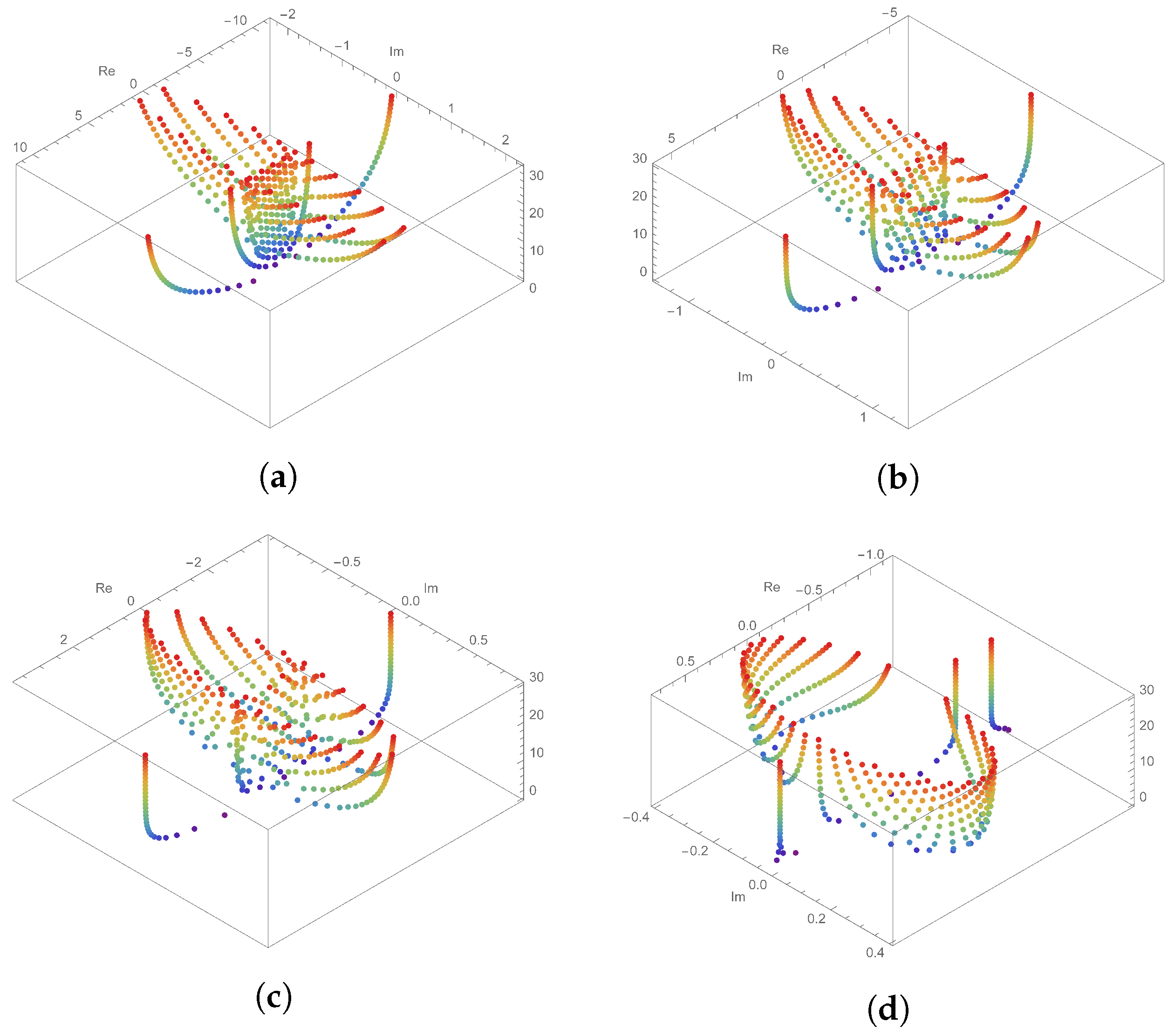
2. Some Properties and Approximate Roots of $(\mathit{p},\mathit{q})$-Cosine Sigmoid Polynomials

In Section 2, we define $(p,q)$-cosine sigmoid polynomials and identify the related properties. To determine the structure of the approximation roots of $(p,q)$-cosine sigmoid polynomials, we fixed the values of $p,y$ and changed the value of q to confirm the particular properties. Furthermore, self-similar properties were identified using iterate functions and Newton algorithms. Figure 1, Figure 2, Figure 3 and Figure 4 and

Table 1. Approximate real zeros of ${}_C{\mathcal{S}}_{n,0.9,0.8}(x,2)$.

n	30	40	50	60
	$-11.1024$	$-11.3194$	$-11.3862$	$-11.4068$
	$-3.61012$	$-3.66856$	$-3.68654$	$-3.69208$
	$-2.30048$	$-2.47562$	$-1.72693$	$-2.48904$
	$-1.2929$	$-2.04704$	$-0.697579$	$-1.41662$
	$-0.286054$	$-0.992877$		$-0.404792$
	0.729155	0.00704653	0.303158	0.604624
	1.82395	1.04214	1.36616	1.70358
	2.06903	2.146	3.68302	2.38741
	3.57276	3.65711	11.383	3.691
	11.0688	11.3091		11.4058

and

Table 2. Approximate real zeros of ${}_C{\mathcal{S}}_{n,0.9,0.1}(x,2)$.

n	30	40	50	60
	$-1$	$-1$	$-1$	$-1$
	$-0.711465$	$-0.711465$	$-0.711465$	$-0.711466$
	0.399349	0.405326	0.401946	0.532724
	0.711465	0.711465	0.711465	0.711465

were obtained using Mathematica.

Definition 11.

Let $x,y\in \mathbb{R}$ with $0<|p/q|<1$. Then, we define $(p,q)$-cosine sigmoid polynomials as

$${\displaystyle \sum _{n=0}^{\infty }}{}_C{\mathcal{S}}_{n,p,q}(x,y)\frac{t^n}{{\left[n\right]}_{p,q}!}=\frac{1}{1+e_{p,q}(-t)}{e}_{p,q}\left(tx\right)CO{S}_{p,q}\left(ty\right).$$

Theorem 1.

For $0<|p/q|<1$, we obtain

$${}_C{\mathcal{S}}_{n,p,q}(x,y)={\displaystyle \sum _{k=0}^n}{\left[\begin{array}{c}n\\ k\end{array}\right]}_{p,q}{\mathcal{S}}_{n-k,p,q}{C}_{k,p,q}(x,y),$$

where ${\sum }_{n=0}^{\infty }{C}_{n,p,q}(x,y)\frac{t^n}{{\left[n\right]}_{p,q}!}=e_{p,q}\left(tx\right)CO{S}_{p,q}\left(ty\right)$ and ${\mathcal{S}}_{n,p,q}$ is the $(p,q)$-sigmoid numbers; see [18].

Proof. 

From generating functions of $(p,q)$-sigmoid numbers and $C_{n,p,q}(x,y)$, we obtain a relation as the following.

$${\displaystyle \sum _{n=0}^{\infty }}{}_C{\mathcal{S}}_{n,p,q}(x,y)\frac{t^n}{{\left[n\right]}_{p,q}!}={\displaystyle \sum _{n=0}^{\infty }}{\mathcal{S}}_{n,p,q}\frac{t^n}{{\left[n\right]}_{p,q}!}{\displaystyle \sum _{n=0}^{\infty }}{C}_{n,p,q}(x,y)\frac{t^n}{{\left[n\right]}_{p,q}!}.$$

(2)

Using Cauchy product in (2), we find

$${\displaystyle \sum _{n=0}^{\infty }}{}_C{\mathcal{S}}_{n,p,q}(x,y)\frac{t^n}{{\left[n\right]}_{p,q}!}={\displaystyle \sum _{n=0}^{\infty }}\left({\displaystyle \sum _{k=0}^n}{\left[\begin{array}{c}n\\ k\end{array}\right]}_{p,q}{\mathcal{S}}_{n-k,p,q}{C}_{k,p,q}(x,y)\right)\frac{t^n}{{\left[n\right]}_{p,q}!},$$

which immediately provides the required result. □

Theorem 2.

For $x,y\in \mathbb{R}$, we derive

$$C_{n,p,q}(x,y)-{}_C{\mathcal{S}}_{n,p,q}(x,y)={\displaystyle \sum _{k=0}^n}{\left[\begin{array}{c}n\\ k\end{array}\right]}_{p,q}{(-1)}^{n-k}{p}^{\left(\genfrac{}{}{0pt}{}{n-k}{2}\right)}{}_C{\mathcal{S}}_{k,p,q}(x,y).$$

Proof. 

Suppose that $e_{p,q}(-t)\ne -1$. From generating function of $(p,q)$-sigmoid polynomials, we have

$${\displaystyle \sum _{n=0}^{\infty }}{}_C{\mathcal{S}}_{n,p,q}(x,y)\frac{t^n}{{\left[n\right]}_{p,q}!}(1+e_{p,q}(-t))={\displaystyle \sum _{n=0}^{\infty }}{C}_{n,p,q}(x,y)\frac{t^n}{{\left[n\right]}_{p,q}!}.$$

(3)

The left-hand side of (2) can be transformed as

$$\begin{array}{l}{\displaystyle \sum _{n=0}^{\infty }}{}_C{\mathcal{S}}_{n,p,q}(x,y)\frac{t^n}{{\left[n\right]}_{p,q}!}(1+e_{p,q}(-t))\\ ={\displaystyle \sum _{n=0}^{\infty }}\left({}_C{\mathcal{S}}_{n,p,q}(x,y)+{\displaystyle \sum _{k=0}^n}{\left[\begin{array}{c}n\\ k\end{array}\right]}_{p,q}{(-1)}^{n-k}{p}^{\left(\genfrac{}{}{0pt}{}{n-k}{2}\right)}{}_C{\mathcal{S}}_{k,p,q}(x,y)\right)\frac{t^n}{{\left[n\right]}_{p,q}!}.\end{array}$$

(4)

Comparing the coefficients of the right-hand side of (3) and the right-hand side of (4), we obtain the desired result. □

In [19], we note

$${p,}_q{C}_{n-1,p,q}(x,y)={\displaystyle \sum _{k=0}^n}{\left[\begin{array}{c}n\\ k\end{array}\right]}_{p,q}{p}^{\left(\genfrac{}{}{0pt}{}{n-k}{2}\right)}{}_C{B}_{k,p,q}(x,y)-{}_C{B}_{n,p,q}(x,y),$$

(5)

where ${}_C{B}_{n,p,q}(x,y)$ is the $(p,q)$-cosine Bernoulli polynomials.

Corollary 1.

From $C_{n,p,q}(x,y)$ of Theorem 2 and (5), the following holds

$$\begin{array}{l}{\displaystyle \sum _{k=0}^n}{\left[\begin{array}{c}n+1\\ k\end{array}\right]}_{p,q}{p}^{\left(\genfrac{}{}{0pt}{}{n-k+1}{2}\right)}{}_C{B}_{k,p,q}(x,y)-{[n+1]}_{p,q}{}_C{\mathcal{S}}_{n,p,q}(x,y)\\ ={\displaystyle \sum _{k=0}^n}{\left[\begin{array}{c}n\\ k\end{array}\right]}_{p,q}{(-1)}^{n-k}{p}^{\left(\genfrac{}{}{0pt}{}{n-k}{2}\right)}{}_C{\mathcal{S}}_{k,p,q}(x,y),\end{array}$$

where ${}_C{B}_{n,p,q}(x,y)$ is the $(p,q)$-cosine Bernoulli polynomials; see [19].

Theorem 3.

Let $a,b$ be any integers. Then, we find

$$\begin{array}{l}{\displaystyle \sum _{k=0}^n}{\left[\begin{array}{c}n\\ k\end{array}\right]}_{p,q}{a}^{n-k}{b}^k{}_C{\mathcal{S}}_{n-k,p,q}\left(\frac{x}{a},\frac{y}{a}\right){}_C{\mathcal{S}}_{k,p,q}\left(\frac{X}{b},\frac{Y}{b}\right)\\ ={\displaystyle \sum _{k=0}^n}{\left[\begin{array}{c}n\\ k\end{array}\right]}_{p,q}{b}^{n-k}{a}^k{}_C{\mathcal{S}}_{n-k,p,q}\left(\frac{x}{b},\frac{y}{b}\right){}_C{\mathcal{S}}_{k,p,q}\left(\frac{X}{a},\frac{Y}{a}\right).\end{array}$$

Proof. 

Substituting $at$ and $bt$ instead of t in the definition of $(p,q)$-cosine sigmoid polynomials, we find

$$\begin{array}{l}\frac{1}{1+e_{p,q}(-at)}{e}_{p,q}\left(tx\right)CO{S}_{p,q}\left(ty\right)\frac{1}{1+e_{p,q}(-bt)}{e}_{p,q}\left(tX\right)CO{S}_{p,q}\left(tY\right)\\ ={\displaystyle \sum _{n=0}^{\infty }}{a}^n{}_C{\mathcal{S}}_{n,p,q}\left(\frac{x}{a},\frac{y}{a}\right)\frac{t^n}{{\left[n\right]}_{p,q}!}{\displaystyle \sum _{n=0}^{\infty }}{b}^n{}_C{\mathcal{S}}_{n,p,q}\left(\frac{X}{b},\frac{Y}{b}\right)\frac{t^n}{{\left[n\right]}_{p,q}!}\\ ={\displaystyle \sum _{n=0}^{\infty }}\left({\displaystyle \sum _{k=0}^n}{\left[\begin{array}{c}n\\ k\end{array}\right]}_{p,q}{a}^{n-k}{b}^k{}_C{\mathcal{S}}_{n-k,p,q}\left(\frac{x}{a},\frac{y}{a}\right){}_C{\mathcal{S}}_{k,p,q}\left(\frac{X}{b},\frac{Y}{b}\right)\right)\frac{t^n}{{\left[n\right]}_{p,q}!},\end{array}$$

(6)

and

$$\begin{array}{l}\frac{1}{1+e_{p,q}(-bt)}{e}_{p,q}\left(tx\right)CO{S}_{p,q}\left(ty\right)\frac{1}{1+e_{p,q}(-at)}{e}_{p,q}\left(tX\right)CO{S}_{p,q}\left(tY\right)\\ ={\displaystyle \sum _{n=0}^{\infty }}\left({\displaystyle \sum _{k=0}^n}{\left[\begin{array}{c}n\\ k\end{array}\right]}_{p,q}{b}^{n-k}{a}^k{}_C{\mathcal{S}}_{n-k,p,q}\left(\frac{x}{b},\frac{y}{b}\right){}_C{\mathcal{S}}_{k,p,q}\left(\frac{X}{a},\frac{Y}{a}\right)\right)\frac{t^n}{{\left[n\right]}_{p,q}!}.\end{array}$$

(7)

From (6) and (7), we complete the proof of Theorem 3. □

Based on the above Theorems 1 and 2, several ${}_C{\mathcal{S}}_{n,p,q}(x,y)$ are obtained as follows:

$$\begin{array}{l}{}_C{\mathcal{S}}_{0,p,q}(x,y)=\frac{1}{2}\\ {}_C{\mathcal{S}}_{1,p,q}(x,y)=\frac{1}{4}(1+2x)\\ {}_C{\mathcal{S}}_{2,p,q}(x,y)=\frac{1}{8}(q+p(-1+2x+4x^2)+2q(x-2y^2))\\ {}_C{\mathcal{S}}_{3,p,q}(x,y)=\frac{1}{16}(p^3-2p^{2}q-2p{q}^2+q^3-2p^{3}x+2q^{3}x+4p^3{x}^2+4p^{2}q{x}^2+4p{q}^2{x}^2\\ +8p^3{x}^3)-\frac{1}{4}q(p^2+pq+q^2)(1+2x)y^2\\ \cdots .\end{array}$$

Here, we can see the structures of the approximation roots shown by varying q, as shown in Figure 1. Let us fix $0\le n\le 30$, $p=0.9$ and $y=2$. The upper left figure (a) in Figure 1 shows the structure of approximation roots under $q=0.8$. The upper right figure (b) is when $q=0.7$. The condition of the figure on the lower left (c) is $q=0.6$ and the condition of the figure on the lower right (d) is $q=0.1$. Figure 1 shows ${}_C{\mathcal{S}}_{n,0.9,q}(x,2)$ when fixed at $p,y$, and it can be inferred that the structure of approximation roots ${}_C{\mathcal{S}}_{n,p,q}(x,y)$ changes from oval to circular form as q becomes smaller. It can also be seen that the number of real roots among the approximation roots decreases as q becomes smaller.

It can also be seen that the number of real roots among the approximation roots decreases as q becomes smaller. It can also be inferred that as n increases and q decreases, the number of real roots decreases and has constant values.

Table 1 shows the value of the real roots in the upper right figure in Figure 1. Table 1 is the value of real roots of $(p,q)$-cosine sigmoid polynomials, which appears with changes in n when fixed at $p=0.9,q=0.8$, and $y=2$.

In Table 1 we can see that even if n increases, there are real roots near the absolute values of 11 and 3. The structures of the approximation roots ${}_C{\mathcal{S}}_{n,0.9,0.8}(x,2)$ appear based on Table 1 and can be seen in Figure 2. The left figure of Figure 2a is the structure of approximation roots when $n=30$, the middle (b) is $n=40$, and the right (c) is the structure of approximation roots when $n=50$. From Figure 1 and Figure 2, and Table 1, we can make several estimations of the picture below on the right side of Figure 1. In other words, it is assumed that the real roots will contain a certain value and the structure of imaginary roots will change from an oval to a circular shape.

Table 2 below is fixed to $p=0.9,q=0.1,y=2$, and the value of approximate real roots of ${}_C{\mathcal{S}}_{n,0.9,0.1}(x,2)$ appears when changing the value of n. Here, we can guess as follows.

Corollary 2.

Fix $p=0.9,q=0.1,y=2$, and as the value of n increases, the approximate real roots of ${}_C{\mathcal{S}}_{n,0.9,0.1}(x,2)$ necessarily includes $-1$ and $0.711465$.

Figure 3 shows the results of a more changed value of q based on the lower right figure in Figure 1. The lower right figure (d) in Figure 1 shows under conditions of $p=0.9,q=0.1,y=2,n=30$, ${}_C{\mathcal{S}}_{n,p,q}(x,y)$ appears to have approximate imaginary roots in the circular position, except for the four approximate real roots. Based on these experimental results, further changes in the value of n can be seen in Figure 3. The red dots in Figure 3 are the approximate imaginary roots of ${}_C{\mathcal{S}}_{n,0.9,0.1}(x,2)$, the blue lines represent the circles closest to the approximate imaginary roots, and the blue dots are the circle’s centers. The left figure (a) in Figure 3 is when $n=50$, the middle figure (b) is when $n=55$, and the right figure (c) is when $n=60$.

Based on Figure 3, we can make the following assumption.

Corollary 3.

The position of approximate imaginary roots of ${}_C{\mathcal{S}}_{n,0.9,0.1}(x,2)$ excluding the approximate real roots are approximated in circular form as n increases.

The following Figure 4 shows the plot using Newton’s method (see [10,20]) when $p=0.9,q=0.8$, and $y=2$. The left figure (a) in Figure 4 is the polynomial ${}_C{\mathcal{S}}_{4,0.9,0.8}(x,2)=0.0179535-0.228746x-0.0807077x^2+0.449246x^3+0.265721x^4$, the middle figure (b) is ${}_C{\mathcal{S}}_{5,0.9,0.8}(x,2)=0.0557219+0.0471837x-0.318265x^2-0.0791739x^3+0.34917x^4+0.174339x^5$ and the right figure (c) is the polynomial ${}_C{\mathcal{S}}_{6,0.9,0.8}(x,2)=-0.0211409+0.150057x+0.0672693x^2-0.319923x^3-0.0630557x^4+0.234745x^5+0.102946x^6$. At this point, we can give the range as $-6\le x,y\le 6$ and the iterate is set to 50. Thus, if Newton’s method is used in the polynomial equations above, each imaginary number in the range approaches the approximate root with different values depending on the polynomial, so these are all marked in different colors.

The figure (a) on the left in Figure 4 represents areas that go towards the values of $-1.4836,-0.922691,0.0773267$, and $0.638295$ in red, purple, yellow, and light blue, respectively. Similarly, the figure (b) in the middle represents regions going to $-1.42568-0.132627i,-1.42568+0.132627i,-0.390578,0.619555-0.123713i,0.619555+0.123713i$ in different colors, and the figure (c) on the right represents regions going to $-1.55365-0.308743i,-1.55365+0.308743i,-0.861364,0.138021,0.775177-0.295858i$, $0.775177+0.295858i$ in different colors.

Here, we can make the following assumption.

Corollary 4.

Using Newton’s method, the boundaries of the areas of ${}_C{\mathcal{S}}_{n,0.9,0.8}(x,2)$ heading to the root, all have self-similarity properties.

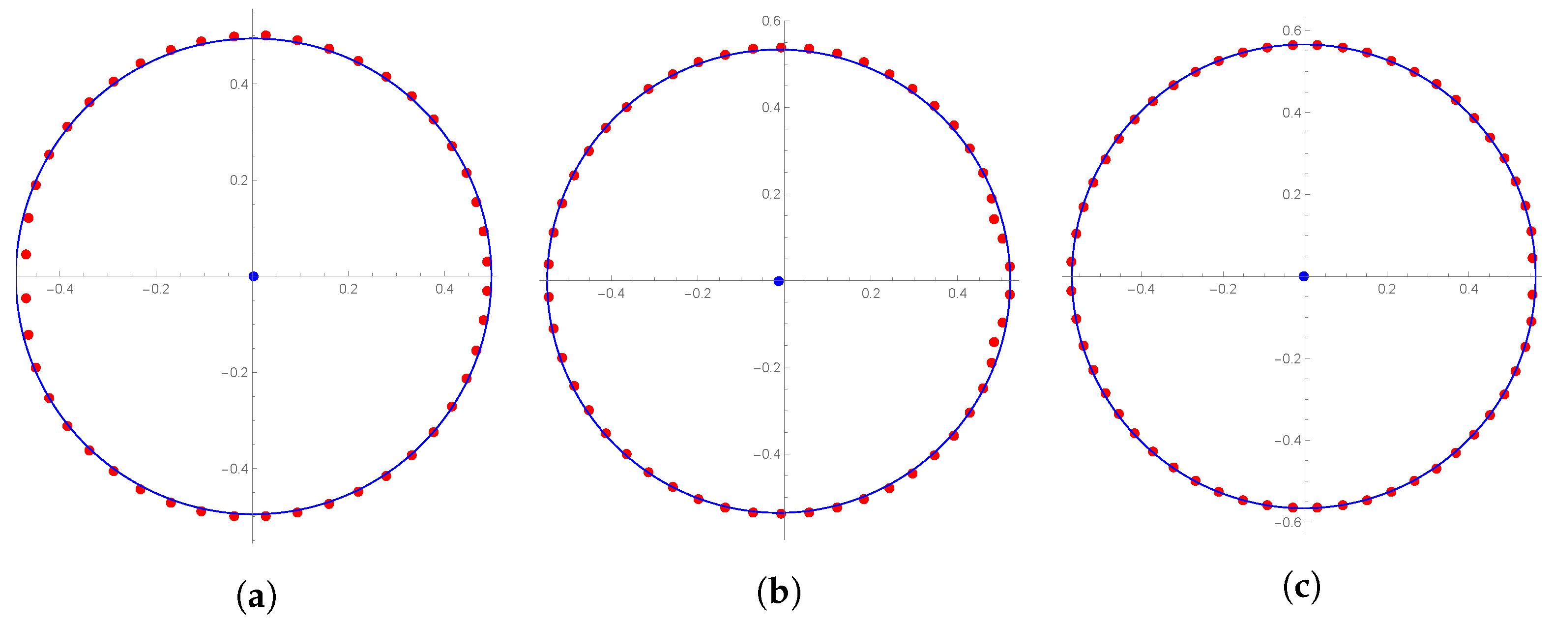
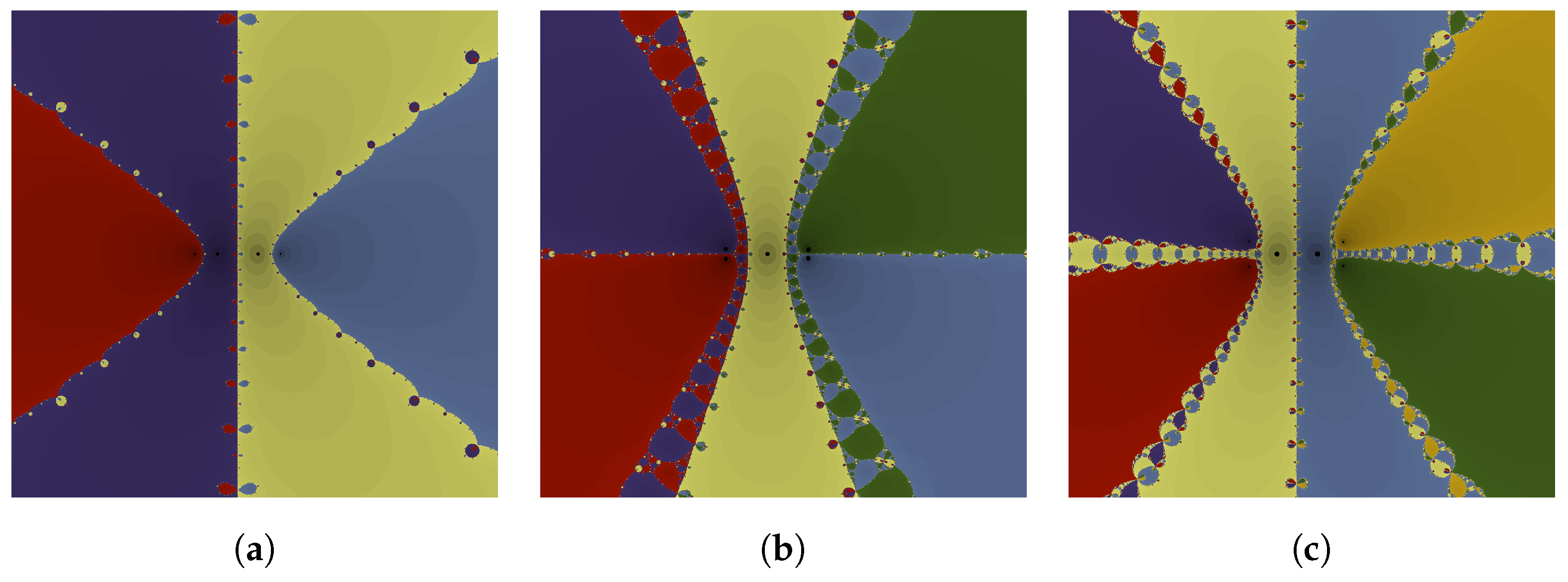
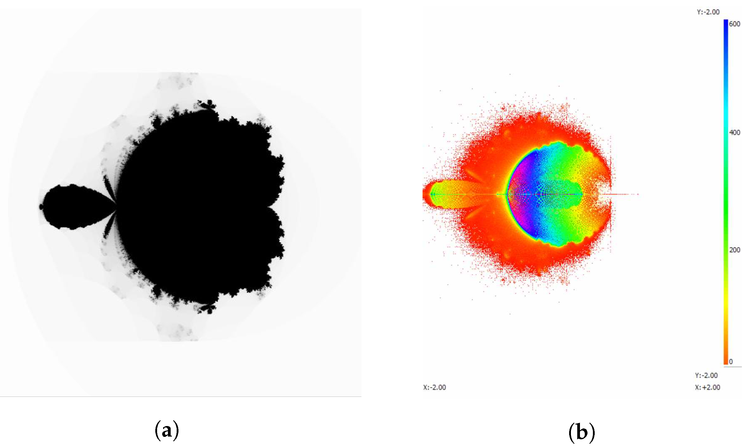
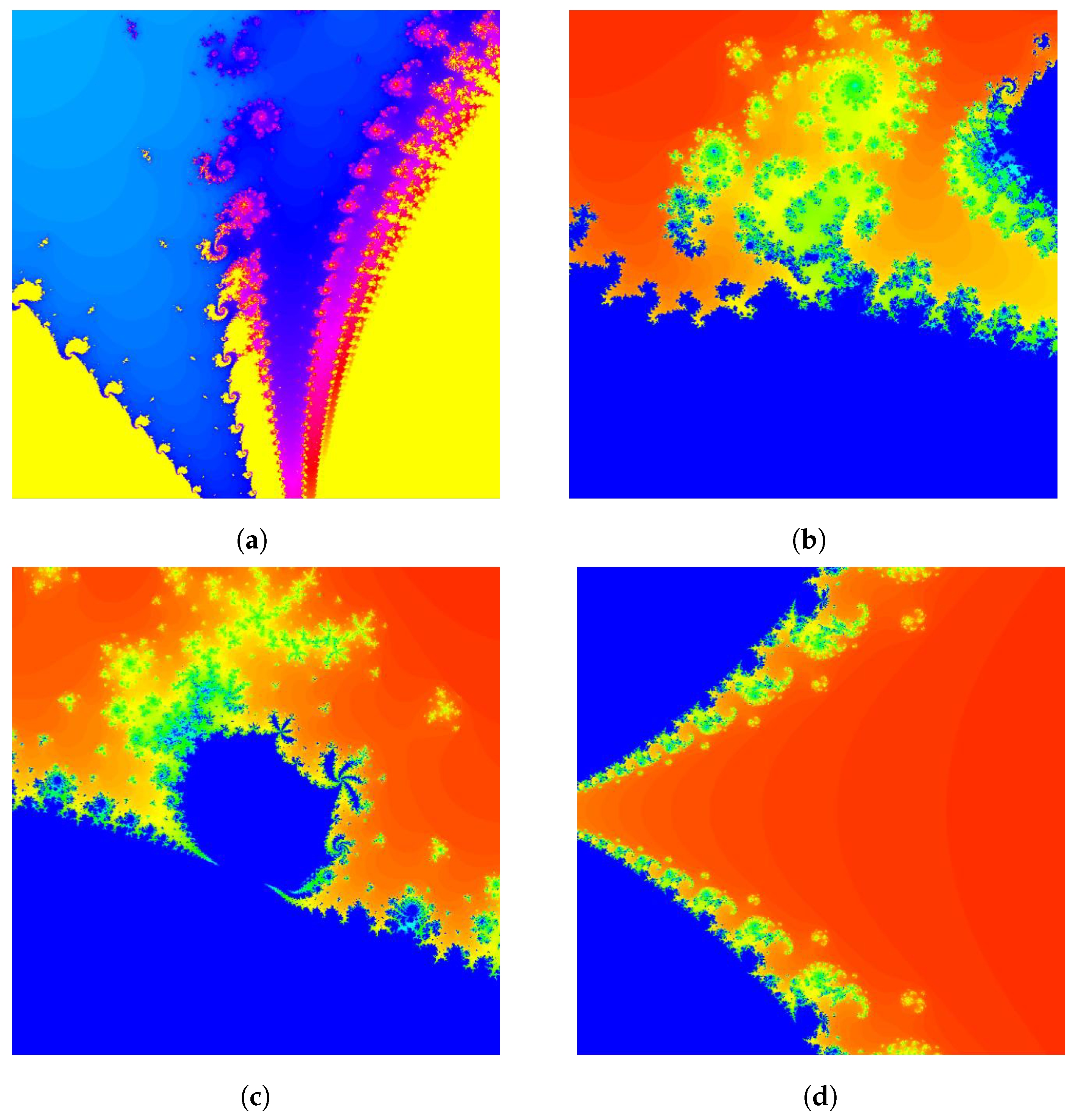
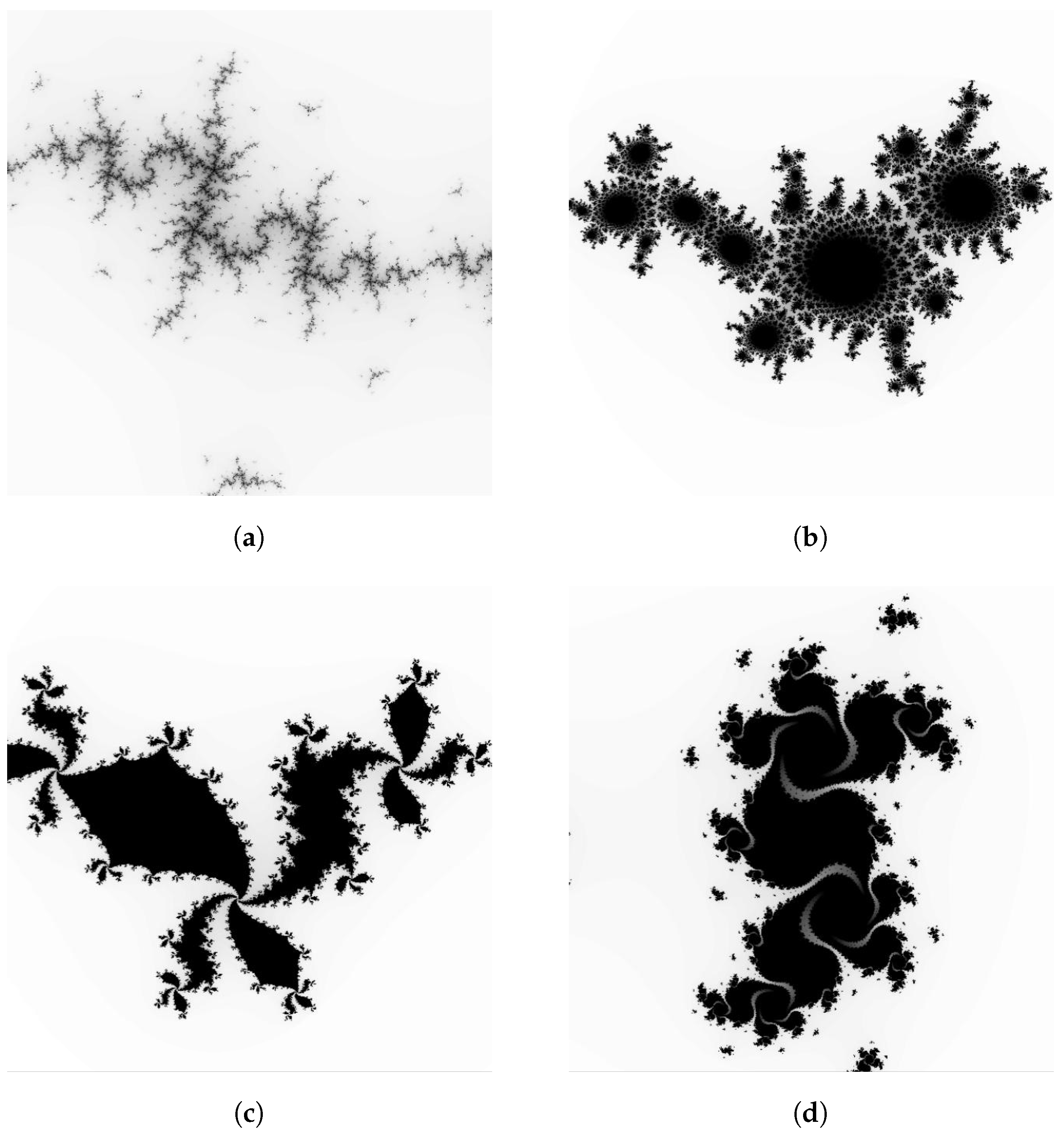
3. Some Fractal Figures and Properties of $(\mathit{p},\mathit{q})$-Sine Sigmoid Polynomials

In Section 3, we define the $(p,q)$-sine sigmoid polynomials and use the properties of $(p,q)$-trigonometric functions to find special properties of $(p,q)$-sine sigmoid polynomials. Furthermore, the values of $q,y$ are fixed and the Mandelbrot and Julia sets according to the change in p are found to confirm their special properties. Figure 5, Figure 6, Figure 7 and Figure 8 are obtained using the C program.

Definition 12.

Let $x,y\in \mathbb{R}$. Then, we define $(p,q)$-sine sigmoid polynomials as follows.

$${\displaystyle \sum _{n=0}^{\infty }}{}_S{\mathcal{S}}_{n,p,q}(x,y)\frac{t^n}{{\left[n\right]}_{p,q}!}=\frac{1}{1+e_{p,q}(-t)}{e}_{p,q}\left(tx\right)SI{N}_{p,q}\left(ty\right).$$

Theorem 4.

For $|p/q|<1$, we derive

$$\begin{gathered} {\mathcal{S}}_{n,p,q}\left(x\right)={\displaystyle \sum _{k=0}^{\left[\frac{n-1}{2}\right]}}{\left[\begin{array}{c}n\\ 2k+1\end{array}\right]}_{p,q}{(-1)}^k{p}^{(2k+1)k}{y}^{2k+1}{}_S{\mathcal{S}}_{n-(2k+1),p,q}(x,y) \\ +{\displaystyle \sum _{k=0}^{\left[\frac{n}{2}\right]}}{\left[\begin{array}{c}n\\ 2k\end{array}\right]}_{p,q}{(-1)}^k{p}^{(2k-1)k}{y}^{2k}{}_C{\mathcal{S}}_{n-k,p,q}(x,y), \end{gathered}$$

where $\left[x\right]$ is the greatest integer not exceeding x and ${\mathcal{S}}_{n,p,q}\left(x\right)$ is the $(p,q)$-sigmoid polynomials.

Proof. 

To use $si{n}_{p,q}\left(x\right)SI{N}_{p,q}\left(x\right)+co{s}_{p,q}\left(x\right)CO{S}_{p,q}\left(x\right)=1$, we note

$$si{n}_{p,q}\left(x\right)={\displaystyle \sum _{n=0}^{\infty }}{(-1)}^n{p}^{(2n+1)n}\frac{x^{2n+1}}{{[2n+1]}_{p,q}!},co{s}_{p,q}\left(x\right)={\displaystyle \sum _{n=0}^{\infty }}{(-1)}^n{p}^{(2n-1)n}\frac{x^{2n}}{{\left[2n\right]}_{p,q}!}.$$

Multiplying $si{n}_{p,q}\left(ty\right)$ in the generating function of $(p,q)$-sine sigmoid polynomials, we find

$$\begin{array}{l}{\displaystyle \sum _{n=0}^{\infty }}{}_S{\mathcal{S}}_{n,p,q}(x,y)\frac{t^n}{{\left[n\right]}_{p,q}!}si{n}_{p,q}\left(ty\right)\\ ={\displaystyle \sum _{n=0}^{\infty }}\left({\displaystyle \sum _{k=0}^{\left[\frac{n-1}{2}\right]}}{\left[\begin{array}{c}n\\ 2k+1\end{array}\right]}_{p,q}{(-1)}^k{p}^{(2k+1)k}{y}^{2k+1}{}_S{\mathcal{S}}_{n-(2k+1),p,q}(x,y)\right)\frac{t^n}{{\left[n\right]}_{p,q}!}\\ =\frac{1}{1+e_{p,q}(-t)}{e}_{p,q}\left(tx\right)SI{N}_{p,q}\left(ty\right)si{n}_{p,q}\left(ty\right).\end{array}$$

(8)

Furthermore, we can find the following equation using the similar way of (8).

$$\begin{array}{l}{\displaystyle \sum _{n=0}^{\infty }}{}_C{\mathcal{S}}_{n,p,q}(x,y)\frac{t^n}{{\left[n\right]}_{p,q}!}{\displaystyle \sum _{n=0}^{\infty }}{(-1)}^n{p}^{(2n-1)n}{y}^{2n}\frac{t^{2n}}{{\left[2n\right]}_{p,q}!}\\ ={\displaystyle \sum _{n=0}^{\infty }}\left({\displaystyle \sum _{k=0}^{\left[\frac{n}{2}\right]}}{\left[\begin{array}{c}n\\ 2k\end{array}\right]}_{p,q}{(-1)}^k{p}^{(2k-1)k}{y}^{2k}{}_C{\mathcal{S}}_{n-k,p,q}(x,y)\right)\frac{t^n}{{\left[n\right]}_{p,q}!}\\ =\frac{1}{1+e_{p,q}(-t)}{e}_{p,q}\left(tx\right)CO{S}_{p,q}\left(ty\right)co{s}_{p,q}\left(ty\right).\end{array}$$

(9)

From (8) and (9), we find

$$\begin{array}{l}\frac{1}{1+e_{p,q}(-t)}{e}_{p,q}\left(tx\right)\left(SI{N}_{p,q}\left(ty\right)si{n}_{p,q}\left(ty\right)+CO{S}_{p,q}\left(ty\right)co{s}_{p,q}\left(ty\right)\right)\\ ={\displaystyle \sum _{n=0}^{\infty }}{\mathcal{S}}_{n,p,q}\left(x\right)\frac{t^n}{{\left[n\right]}_{p,q}!}\\ ={\displaystyle \sum _{n=0}^{\infty }}\left({\displaystyle \sum _{k=0}^{\left[\frac{n-1}{2}\right]}}{\left[\begin{array}{c}n\\ 2k+1\end{array}\right]}_{p,q}{(-1)}^k{p}^{(2k+1)k}{y}^{2k+1}{}_S{\mathcal{S}}_{n-(2k+1),p,q}(x,y)\right)\frac{t^n}{{\left[n\right]}_{p,q}!}\\ +{\displaystyle \sum _{n=0}^{\infty }}\left({\displaystyle \sum _{k=0}^{\left[\frac{n}{2}\right]}}{\left[\begin{array}{c}n\\ 2k\end{array}\right]}_{p,q}{(-1)}^k{p}^{(2k-1)k}{y}^{2k}{}_C{\mathcal{S}}_{n-k,p,q}(x,y)\right)\frac{t^n}{{\left[n\right]}_{p,q}!}.\end{array}$$

Therefore, we look at the required result. □

Corollary 5.

Set $p=1$ and $y=1$ in Theorem 4. Then, the following holds

$$\begin{array}{ll}{\mathcal{S}}_{n,q}\left(x\right)=& {\displaystyle \sum _{k=0}^{\left[\frac{n-1}{2}\right]}}{\left[\begin{array}{c}n\\ 2k+1\end{array}\right]}_q{(-1)}^k{}_S{\mathcal{S}}_{n-(2k+1),q}(x,1)\\ & +{\displaystyle \sum _{k=0}^{\left[\frac{n}{2}\right]}}{\left[\begin{array}{c}n\\ 2k\end{array}\right]}_q{(-1)}^k{}_C{\mathcal{S}}_{n-k,q}(x,1),\end{array}$$

where $\left[x\right]$ is the greatest integer not exceeding x and ${\mathcal{S}}_{n,q}\left(x\right)$ is the q-sigmoid polynomials.

Theorem 5.

Let $a,b$ be non-negative integers. Then, we have

$$\begin{array}{l}{\displaystyle \sum _{k=0}^n}{\left[\begin{array}{c}n\\ k\end{array}\right]}_{p,q}{a}^{n-k}{b}^k{}_C{\mathcal{S}}_{n-k,p,q}(x,y)\left(\frac{x}{a},\frac{y}{a}\right){}_S{\mathcal{S}}_{k,p,q}(x,y)\left(\frac{x}{b},\frac{y}{b}\right)\\ ={\displaystyle \sum _{k=0}^n}{\left[\begin{array}{c}n\\ k\end{array}\right]}_{p,q}{b}^{n-k}{a}^k{}_C{\mathcal{S}}_{n-k,p,q}(x,y)\left(\frac{x}{b},\frac{y}{b}\right){}_S{\mathcal{S}}_{k,p,q}(x,y)\left(\frac{x}{a},\frac{y}{a}\right).\end{array}$$

Proof. 

From the generating functions of $(p,q)$-cosine sigmoid polynomials and $(p,q)$-sine sigmoid polynomials, we can consider

$$A:=\frac{{\left(e_{p,q}\left(tx\right)\right)}^{2}CO{S}_{p,q}\left(ty\right)SI{N}_{p,q}\left(ty\right)}{(1+e_{p,q}(-at))(1+e_{p,q}(-bt))}.$$

The form A can be transformed as

$$\begin{array}{ll}A& =\frac{1}{1+e_{p,q}(-at)}{e}_{p,q}\left(tx\right)CO{S}_{p,q}\left(ty\right)\frac{1}{1+e_{p,q}(-bt)}{e}_{p,q}\left(tx\right)SI{N}_{p,q}\left(ty\right)\\ & ={\displaystyle \sum _{n=0}^{\infty }}\left({\displaystyle \sum _{k=0}^n}{\left[\begin{array}{c}n\\ k\end{array}\right]}_{p,q}{a}^{n-k}{b}^k{}_C{\mathcal{S}}_{n-k,p,q}\left(\frac{x}{a},\frac{y}{a}\right){}_S{\mathcal{S}}_{k,p,q}\left(\frac{x}{b},\frac{y}{b}\right)\right)\frac{t^n}{{\left[n\right]}_{p,q}!},\end{array}$$

and

$$A={\displaystyle \sum _{n=0}^{\infty }}\left({\displaystyle \sum _{k=0}^n}{\left[\begin{array}{c}n\\ k\end{array}\right]}_{p,q}{b}^{n-k}{a}^k{}_C{\mathcal{S}}_{n-k,p,q}\left(\frac{x}{b},\frac{y}{b}\right){}_S{\mathcal{S}}_{k,p,q}\left(\frac{x}{a},\frac{y}{a}\right)\right)\frac{t^n}{{\left[n\right]}_{p,q}!}.$$

From transformed equations, we can see the desired result, which is a symmetric property for mixed $(p,q)$-cosine sigmoid polynomials and $(p,q)$-sine sigmoid polynomials. □

Corollary 6.

Put $a=1$ in Theorem 5. Then, one holds

$${\displaystyle \sum _{k=0}^n}{\left[\begin{array}{c}n\\ k\end{array}\right]}_{p,q}{b}^k{}_C{\mathcal{S}}_{n-k,p,q}(x,y){}_S{\mathcal{S}}_{k,p,q}\left(\frac{x}{b},\frac{y}{b}\right)={\displaystyle \sum _{k=0}^n}{\left[\begin{array}{c}n\\ k\end{array}\right]}_{p,q}{b}^{n-k}{}_C{\mathcal{S}}_{k,p,q}\left(\frac{x}{b},\frac{y}{b}\right){}_S{\mathcal{S}}_{k,p,q}(x,y).$$

Several $(p,q)$-sine sigmoid polynomials are shown in the following.

$$\begin{array}{l}{}_S{\mathcal{S}}_{0,p,q}(x,y)=0,\\ {}_S{\mathcal{S}}_{1,p,q}(x,y)=\frac{y}{2},\\ {}_S{\mathcal{S}}_{2,p,q}(x,y)=\frac{1}{4}(p+q)(1+2x)y,\\ {}_S{\mathcal{S}}_{3,p,q}(x,y)=\frac{1}{8}y(4p^{2}qx(1+x)+4p{q}^{2}x(1+x)+p^3(-1+2x+4x^2)+q^3(1+2x-4y^2)),\\ {}_S{\mathcal{S}}_{4,p,q}(x,y)=\frac{1}{16}(p^3+p^{2}q+p{q}^2+q^3)y(2p^{2}q(-1+2x^2)+2p{q}^2(-1+2x^2)\\ +\frac{1}{16}{p}^3(1-2x+4x^2+8x^3)-q^3(1+2x)(-1+4y^2),\\ \cdots .\end{array}$$

Hereafter, we look at the Mandelbrot set and the Julia set, which can be found based on the above polynomials.

Consider

$$f_{128}:x\mapsto \underset{128}{\underbrace{f\left(f\right(\cdots (f}}\left(x\right)\left)\right)).$$

where $f\left(x\right)={}_S{\mathcal{S}}_{3,0.8,0.9}(x,1)+c=0.868x^2+0.92225x-0.337375+c$.

The Mandelbrot set can be seen in the left picture in Figure 5.

In Figure 5, the figure on the right (b), is an accumulated map of the attracting points that appear under the same conditions. As shown on the left (a), the range of real and imaginary axes is between $-2$ and 2. In addition, the red area can be seen as having very few attracting points, and the blue areas can be seen as having several attracting points. Here, the red area is expressed as having piling up zero attracting points, and the blue area is represented by piling up to 600 attracting points. In the picture on the right in Figure 5, we can see that the blue area appears.

Figure 6 shows the Madelbrot sets that appear differently with changes in p in ${}_S{\mathcal{S}}_{4,p,0.9}(x,1)$ and shows an extended view of the Mandelbrot set of polynomials. Here, we iterate the polynomial 128 times and set the convergence range of upper figures as 4 in the above Figure 6.

The conditions in the upper left figure (a) are $p=0.8$, the range of the real axis is from $0.5525$ to $0.74$, and the range of the imaginary axis is from $0.08875$ to $0.27625$, with the polynomial being $-0.6352-0.831629x+1.06981x^2+0.63104x^3$. The yellow range that appears here is iterated 128 times. The upper right figure (b) shows the condition of $p=0.6$; the range of the real axis is from $-1.6555$ to $-1.28$, and the range of the imaginary axis is from $0.82125$ to $1.19625$. The polynomial here is $-0.393888-0.527158x+0.450158x^2+0.18954x^3$, and we gave the center of the image as $-1.4675+1.00875i$.

Here, the blue range means the polynomial has been iterated 128 times, and the red range means the lowest number of times it has been iterated. The condition of the lower left figure (c) is $p=0.4$, and the convergence range is set to 8. The polynomial in the figure is $-0.241087-0.354814x+0.167713x^2+0.040352x^3$. The center of the image of this figure is $0.80625+2.9575i$, and the point of $2+2.4i$ can be seen moving with a 3-period. The lower right figure (d) is part of the polynomial $-0.150477-0.256541x+0.0481525x^2+0.00374x^3$ that appears when $p=0.2$, and the convergence range is given as 32. We gave the center of the image as $6.45125-0.0025i$, the range of the real axis from $5.70125$ to $7.20125$ and the range of the imaginary axis from $-0.7525$ to $0.7525$.

Figure 7 shows the Julia set and shows the changes in the picture when the offset is given differently in the same polynomial. Here, we can see one of the continent shapes in the left picture changing as the corner, and the area in the shape of the continent becomes smaller as the picture goes to the right. The polynomial in Figure 7 is $0.0790275-0.23493x+0.503685x^2+0.89667x^3$ when $p=0.9,q=0.1$, and $y=3$. The offset in the left picture (a) is $0.66750000-0.3250000i$, the offset in the middle (b) is $0.85500000-0.60000i$, and the offset in the right (c) is $0.840000-0.990000i$. In addition, the range in Figure 7 has the real axis and imaginary axis from $-1.125$ to $1.125$, with the number of iterations being 128.

Figure 8 shows Julia set’s various shapes for ${}_S{\mathcal{S}}_{4,p,0.9}(x,1)$ by setting the number of iterations to 128. The upper left figure (a) shows the condition of $p=0.8$, the range of the real axis from $-2.045$ to $-0.545$ and the range of the imaginary axis from $-0.915$ to $-0.585$. The polynomial here is $-0.6352-0.831629x+1.06981x^2+0.63104x^3$, and the offset is shown if $-0.9-0.5i$. The center of the image is $-1.29-0.165i$. The upper right figure (b) shows the condition of $p=0.6$, the range of the real axis from $-3.79$ to $2.21$, and the range of the imaginary axis from $-3.32$ to $2.68$. The polynomial here is $-0.393888-0.527158x+0.450158x^2+0.18954x^3$ and the offset is shown if $-0.03-1.05i$. The convergence range of upper figures is 4. The lower left figure (c) shows the condition of $p=0.4$, the range of the real axis is from $-6.94$ to $5.06$, and the range of the imaginary axis is from $-6.42$ to $5.58$. The polynomial here is $-0.393888-0.527158x+0.450158x^2+0.18954x^3$ and the offset is shown in $-1.44-3.8i$. The center of the image is $-0.94-0.42i$, and the convergence range is 8. This figure consists of four leaves, and the shape of the top left leaf is the biggest. This shape appears infinitely and repeatedly. The lower right figure (d) shows the polynomial $-0.150477-0.256541x^2+0.00374x^3$, which appears when $p=0.2$, the convergence range is 32 and offset is given as $7.04-4.08i$. Let us give the center of the image as $1.76+0.32i$, the range of the real axis from $14.74$ to $18.26$, and the range of the imaginary axis from $-16.18$ to $16.82$.

4. Conclusions

We defined $(p,q)$-cosine sigmoid polynomials and $(p,q)$-sine sigmoid polynomials and identified the special properties that appear in polynomials, respectively. We also used the program to visualize the properties as p and q change. The values of $p,q$ can be found via a variety of methods, so more research is needed on this, and it is important that fractals for higher-order polynomials are actively studied.

References

1. Chakrabarti, R.; Jagannathan, R. A (p,q)-oscillator realization of two-parameter quantum algebras. J. Phys. A Math. Gen. 1991, 24, L711. [Google Scholar] [CrossRef]
2. Araci, S.; Duran, U.; Acikgoz, M.; Srivastava, H.M. A certain (p,q)-derivative operator and associated divided differences. J. Comput. Theor. Nanosci. 2016, 301. [Google Scholar] [CrossRef] [Green Version]
3. Brodimas, G.; Jannussis, A.; Mignani, R. Two-Parameter Quantum Groups; Preprint; Universita di Roma: Rome, Italy, 1991; Nr. 820. [Google Scholar]
4. Burban, M.; Klimyk, A.U. (P,Q)-differentiation, (P,Q)-integration and (P,Q)-hypergeometric functions related to quantum groups. Integral Transform. Spec. Funct. 1994, 2, 15–36. [Google Scholar] [CrossRef]
5. Corcino, R.B. On (P,Q)-Binomial coefficients. Electron. J. Comb. Number Theory 2008, 8, A29. [Google Scholar]
6. Jagannathan, R.; Rao, K.S. Two-parameter quantum algebras, twin-basic numbers, and associated generalized hypergeometric series. Proceeding of the International Conference on Number Theory and Mathematical Physics, Srinivasa Ramanujan Centre, Kumbakonam, India, 20–21 December 2005. [Google Scholar]
7. Jagannathan, R. (P,Q)-Special functions. arXiv 1998, arXiv:math/9803142v1. [Google Scholar]
8. Kang, J.Y.; Ryoo, C.S. A numerical Investigation on the structure of the zeros of the q-tangent polynomials. In Polynomials-Theory and Application; IntechOpen: London, UK, 2019; pp. 1–18. [Google Scholar]
9. Ryoo, C.S. A numerical investigation on the zeros of the tangent polynomials. J. Appl. Math. Inform. 2014, 32, 315–322. [Google Scholar] [CrossRef]
10. Barnsley, M.F. Fractals Everywhere, 3rd ed.; Academic Press: Boston, MA, USA; San Diego, CA, USA; New York, NY, USA, 1988. [Google Scholar]
11. Han, J.; Moraga, C. The influence of the sigmoid function parameters on the speed of backpropagation learning. Int. Workshop Artif. Neural Netw. 2005, 930, 195–201. [Google Scholar]
12. Han, J.; Wilson, R.S.; Leurgans, S.E. Sigmoidal mixed models for longitudinal data. Stat. Methods Med. Res. 2018, 27, 863–875. [Google Scholar] [CrossRef]
13. Kwan, H.K. Simple sigmoid-like activation function suitable for digital hardware implementation. Stat. Methods Med. Res. 1992, 28, 1379–1380. [Google Scholar] [CrossRef]
14. Kang, J.Y. Some relationships between sigmoid polynomials and other polynomials. J. Appl. Pure. Math. 2019, 1, 57–67. [Google Scholar]
15. Kang, J.Y. Explicit properties of q-sigmoid polynomials combining q-cosine function. J. Appl. Math. Inform. 2021, 39, 541–552. [Google Scholar]
16. Rodrigues, P.S.; Lopes, G.W.; Santos, R.M.; Coltri, E.; Giraldi, G.A. A q-extension of sigmoid functions and the application for enhancement of ultrasound images. Entropy 2019, 21, 430. [Google Scholar] [CrossRef] [PubMed] [Green Version]
17. Kang, J.Y. Some Properties and Distribution of the Zeros of the q-Sigmoid Polynomials. Discret. Dyn. Nat. Soc. 2020, 2020, 4169840. [Google Scholar] [CrossRef]
18. Kang, J.Y. Determination of the properties of (p,q)-sigmoid polynomials and the structure of their roots. In Number Theory and Its Applications; IntechOpen: London, UK, 2020; pp. 1–19. [Google Scholar]
19. Ryoo, C.S.; Kang, J.Y. Structure of approximate roots based on symmetric properties of (p,q)-cosine and (p,q)-sine Bernoulli polynomials. Symmetry 2020, 12, 885. [Google Scholar] [CrossRef]
20. Garcia, F.; Fernandez, A.; Barrallo, J.; Martin, L. Coloring Dynamical Systems in the Complex Plane. Retrieved 21 January 2008. Available online: http://math.unipa.it/grim/Jbarrallo.PDF (accessed on 30 August 2021).
Figure 1. Structures of approximation roots of C S n , 0.9 , q ( x , 2 ) for   q = 0.8 , 0.7 , 0.6 , 0.1 with   0 n 30 . (a) C S n , 0.9 , 0.8 ( x , 2 ) ; (b) C S n , 0.9 , 0.7 ( x , 2 ) ; (c) C S n , 0.9 , 0.6 ( x , 2 ) ; (d) C S n , 0.9 , 0.1 ( x , 2 ) .
Fractalfract 05 00245 g001
Figure 2. The positions of approximation roots of C S n , 0.9 , 0.8 ( x , 2 ) for n = 30 , 40 , 50 . (a) C S 30 , 0.9 , 0.8 ( x , 2 ) ; (b) C S 40 , 0.9 , 0.8 ( x , 2 ) ; (c) C S 50 , 0.9 , 0.8 ( x , 2 ) .
Fractalfract 05 00245 g002
Figure 3. Approximate circles of zeros for C S n , 0.9 , 0.1 ( x , 2 ) for n = 50 , 55 , 60 . (a) C S 50 , 0.9 , 0.1 ( x , 2 ) ; (b) C S 55 , 0.9 , 0.1 ( x , 2 ) ; (c) C S 60 , 0.9 , 0.1 ( x , 2 ) .
Fractalfract 05 00245 g003
Figure 4. C S n , 0.9 , q ( x , 2 ) using Newton’s method for n = 4 , 5 , 6 iterating 50-times. (a) C S 4 , 0.9 , 0.8 ( x , 2 ) ; (b) C S 5 , 0.9 , 0.8 ( x , 2 ) ; (c) C S 6 , 0.9 , 0.8 ( x , 2 ) .
Fractalfract 05 00245 g004
Figure 5. The Madelbrot set and accumulated map of S S 3 , 0.8 , 0.9 ( x , 1 ) iterating 128-times. (a) Mandelbrot set of S S 3 , 0.8 , 0.9 ( x , 1 ) ; (b) accumulated map of S S 3 , 0.8 , 0.9 ( x , 1 ) .
Fractalfract 05 00245 g005
Figure 6. The Madelbrot sets of S S 4 , p , 0.9 ( x , 1 ) when p = 0.8 , 0.6 , 0.4 , 0.2 iterating 128-times. (a) S S 4 , 0.8 , 0.9 ( x , 1 ) ; (b) S S 4 , 0.6 , 0.9 ( x , 1 ) ; (c) S S 4 , 0.4 , 0.9 ( x , 1 ) ; (d) S S 4 , 0.2 , 0.9 ( x , 1 ) .
Fractalfract 05 00245 g006
Figure 7. Julia sets that appear differently depending on offset at S S 4 , 0.9 , 0.1 ( x , 3 ) iterating 128-times. (a) S S 4 , 0.9 , 0.1 ( x , 3 ) , c = 0.66750000 0.3250000 i ; (b) S S 4 , 0.9 , 0.1 ( x , 3 ) , c = 0.85500000 0.60000 i ; (c) S S 4 , 0.9 , 0.1 ( x , 3 ) , c = 0.840000 0.990000 i .
Fractalfract 05 00245 g007
Figure 8. Julia sets of S S 4 , p , 0.9 ( x , 1 ) if   p = 0.8 , 0.6 , 0.4 , 0.2 iterating 128-times. (a) S S 4 , 0.8 , 0.9 ( x , 1 ) , c = 1.44 3.8 i ; (b) S S 4 , 0.6 , 0.9 ( x , 1 ) , c = 1.44 3.8 i ; (c) S S 4 , 0.4 , 0.9 ( x , 1 ) , c = 1.44 3.8 i ; (d) S S 4 , 0.2 , 0.9 ( x , 1 ) , c = 1.44 3.8 i .
Fractalfract 05 00245 g008