Abstract
We investigate Benford’s law in relation to fractal geometry. Basic fractals, such as the Cantor set and Sierpinski triangle are obtained as the limit of iterative sets, and the unique measures of their components follow a geometric distribution, which is Benford in most bases. Building on this intuition, we aim to study this distribution in more complicated fractals. We examine the Laurent coefficients of a Riemann mapping and the Taylor coefficients of its reciprocal function from the exterior of the Mandelbrot set to the complement of the unit disk. These coefficients are 2-adic rational numbers, and through statistical testing, we demonstrate that the numerators and denominators are a good fit for Benford’s law. We offer additional conjectures and observations about these coefficients. In particular, we highlight certain arithmetic subsequences related to the coefficients’ denominators, provide an estimate for their slope, and describe efficient methods to compute them.
1. Introduction
The Mandelbrot set was first introduced and drawn by Brooks and Matelski. By analyzing the family of functions , Douady and Hubbard began the formal mathematical study of the Mandelbrot set as the set of parameters c, for which the orbit of 0 under remains bounded. We study Benford’s law in relation to the Mandelbrot set to both investigate the distribution’s extension to fractal geometry and search for patterns in the Mandelbrot set.
In 1980, Douady and Hubbard were able to prove the connectedness of by constructing a conformal isomorphism
between the complement of the Mandelbrot set and the complement of the closed unit disk [1]. Using the Douady-Hubbard map , we can define related conformal isomorphisms,
where , by setting and . One of the most heavily studied questions in complex dynamics is whether or not is locally connected (MLC). By a theorem of Caratheodory [2], these two maps can be extended continuously to the unit circle if and only if the Mandelbrot set is locally connected. As such, we focus on studying these maps and their respective Laurent and Taylor expansions, as outlined in [3,4], respectively:
In Section 3, we outline the methods [3,4,5] we used to compute the and coefficients. The computation time grows exponentially, so methods of improving computation are explored. Using recursion, we were able to compute the first 7168 coefficients.
In Section 4, we discuss Benford’s law along with statistical testing to determine whether the coefficients obey a Benford distribution. Given a base , a data set is Benford base b if the probability of observing a given leading digit, d, is (see [6,7]).(We can write any positive x as , where is the significand and is an integer. If the probability of observing a significand of is , we say the set is strongly Benford (or frequently just Benford).) In most cases, a data set is demonstrated to be Benford through statistical testing. There are few straightforward proofs for Benfordness, all of which rely heavily on understanding the structure and properties of the data. Well understood sets such as geometric series and the Fibonacci numbers have explicit proofs for Benfordness, but the structure and properties of coefficients we study are still the subject of active research in complex dynamics. Therefore, we rely on statistical testing for our results. We consider the standard distribution and the sequence of the data’s logarithms modulo 1 for our statistical testing, and a standard goodness of fit test demonstrates that the numerators and denominators are a good fit for Benford’s law, while the decimal representations are not.
Section 5 deals with conjecture, observations, and theorems related to the coefficients. Section 5.1 and Section 5.2 are meant to tie together the most important of these that we have found from various authors for the and coefficients, respectively. In Section 5.3, we present new results and conjectures on the and coefficients from our work. Theorem 7 [3,8] states that they are 2-adic rational numbers; in other words, they are of the form , where p is an odd integer. The integer is, by definition, the 2-adic valuation of or . Therefore, we focus on the denominator’s exponents , . Setting , with odd and n fixed; the subsequences , appear to be near-arithmetic progressions. We present the results observed in the following conjecture.
Conjecture 1.
Let m be written as as above, with fixed. Then, the sequence is asymptotically linear, with slope
We also present an efficient way to compute the denominator’s exponents for the cases .
Our work offers a new approach to some classical problems in complex dynamics, and we do this through our statistical testing. These coefficients have been studied extensively, so we compile relevant observations from disparate authors to use as a basis for offering new conjectures and results. The idea of studying Benford’s law in complex dynamics and fractal sets is also original; to our knowledge, no other authors have attempted to study Benford’s law in this setting. Our approach offers both a new and unique way to study important series in complex dynamics, and it provides motivation for number theorists and statisticians to study Benford’s law in the new field of data, namely fractal sets.
2. Preliminaries in Complex Dynamics
We give a brief introduction to complex dynamics. For more detailed proofs see [9,10].
Let be a rational map. The Julia set associated to the map f may be defined as the closure of the set of repelling periodic points of f. For a rational map of degree 2 or higher, the Julia set is non-empty. We now restrict our attention to polynomial maps of degree , which have a superattracting fixed point at infinity. We can thus define the filled Julia set as the complement of the basin of the attraction of infinity:
Making use of the above, it is possible to redefine as the boundary of the filled Julia set.
Lemma 1.
Let f be a polynomial of degree . The filled Julia set is compact, with boundary equal to the Julia set. The complement is connected and equal to the basin of attraction of the point ∞.
It follows that the Julia set of a polynomial f is precisely the boundary of the basin of attraction .
We may now characterize the connectedness of . This is determined entirely by the activity of the critical points of f.
Theorem 1.
The Julia set for a polynomial of degree is connected if and only if the filled Julia set contains every critical point of f.
The Mandelbrot Set
We now focus primarily on the family of quadratic functions of the form . Since has a single critical point 0, it follows from Theorem 1 that is connected if and only if the orbit is bounded. This motivates the following definition of the Mandelbrot set, .
Definition 1.
is the set of all the parameters such that the Julia set is connected. Equivalently, is the set of all the c such that the orbit of 0 under remains bounded:
Remark 1.
It is possible to generalize this definition and most of the following results to the family of unicritical degree d polynomials , where d is an integer . In this case, is called the multibrot set of degree d. For simplicity, we focus only on , which has historically been the object of greatest interest. For more information on , see [3,8].
It is possible to demonstrate that the interior of is nonempty. We utilized an escape time algorithm and computer graphics to obtain the visualization of in presented in Figure 1.
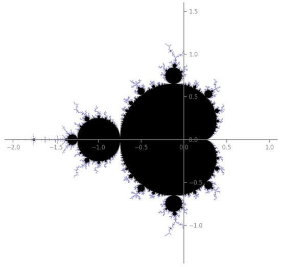
Figure 1.
The Mandelbrot set in the complex plane.
When the first computer images of were generated, Benoit Mandelbrot observed small regions that appeared to be separate from the main cardioid, and conjectured that was disconnected, which was later disproved.
Theorem 2
(Douady, Hubbard). The Mandelbrot set is connected.
This result was first proved by Douady and Hubbard [1] by explicitly constructing a conformal isomorphism . Douady and Hubbard’s proof is significant not only for the result, but also since it provides an explicit formula for the uniformization of the complement of the Mandelbrot set.
A large amount of research has been devoted to the local connectivity of the Mandelbrot set, which is generally regarded as one of the most important open problems in complex dynamics. We recall that a set A in a topological space X is locally connected at if for every open set containing p, there is an open subset U with such that is connected. The set A is said to be locally connected if it is locally connected at p for all .
As above, let be the conformal isomorphism constructed by Douady and Hubbard; notice that the map is the Riemann mapping function of . We consider it the Laurent expansion at ∞
Another possibility is to consider , which is the Riemann mapping of the bounded domain . We have the corresponding Taylor expansion for at the origin:
For the general Multibrot set , we refer to the coefficients with the notation and . To underline the importance of these maps, we reference a lemma from Caratheodory [2].
Theorem 3
(Caratheodory’s continuity lemma). Let be a simply connected domain and a function f maps onto G via a conformal isomorphism. Then f has a continuous extension to if and only if the boundary of G is locally connected.
Therefore, if the map or the map f can be extended continuously to the unit circle , then is locally connected. To demonstrate this extension, it would be sufficient to prove that one of the two series converges uniformly on .
There have been numerous attempts to prove this result. For example, Ewing and Schober demonstrated that the inequality < 1/m holds for every m < . A bound of the type would lead to the desired result; however, this would imply that the extension of is Hölder continuous, which does not happen, as expressed in [11]. Proving that K/(m (m)) would prove that the series converges absolutely; however, modern computations suggest that such a bound does not exist [11]. Therefore, the MLC conjecture and its consequences remain the object of study.
Remark 2
(Consequences of local connectedness). This paper tackles problems related to the behaviour of the coefficients and , with the ultimate aim of improving the state-of-art on the local connectedness of . In this section, we highlight the importance of this property of . In particular, it implies a conjecture known as the Density of Hyperbolicity. A hyperbolic component is an interior connected component of , in which the sequences have an attracting periodic cycle of period p. The Density of Hyperbolicity conjecture states that these are the only interior regions of . Another consequence of MLC is related to a topologically equivalent description of . In particular, the boundary of the Mandelbrot set can be identified with the unit circle under a specific relation ∼, known as the abstract Mandelbrot set [12]. More information and other implications of MLC and the Density of Hyperbolicity may be found in [1,13].
3. Algorithms and Complexity
There are algorithms to compute both the coefficients and . While these algorithms work for a generic degree , we focus on , which is historically the most interesting case, since it is the one associated with . For simplicity, we denote and . The behavior for other values is similar. Derivations for the explicit form of the coefficients may be found in [3]. Derivations for the explicit form of the coefficients may be found in [4]. There is also a formula to switch between the coefficients, outlined in [14].
Theorem 4.
Let and . Then
where the sum is over all non-negative indices such that
and is the generalized binomial coefficient
The coefficients can be obtained from the using the formula
or they can be directly calculated as in the following theorem.
Theorem 5.
Let and . Then
where the sum is over all non-negative indices such that
and is the generalized binomial coefficient
While the above theorems give the explicit forms of the coefficients, the following theorem provides a recursive method to find , which is more suitable for computers. Once we find , we can apply the relationship between and outlined in Theorem 4 to find . More details can be found in [5].
Theorem 6.
Let and . Then
where the following holds true.
Example 1.
For example, to calculate the first several coefficients, we can use Theorem 6 to obtain:
since
3.1. Direct Computation
Our initial algorithm to generate these coefficients was to directly compute them, and we include our original methodology for reference as we cross checked our results. Most of the data was generated through the recursive algorithm, and details are provided in Section 3.2.
We wrote a program in Python to compute and based on the formulas given in Theorems 4 and 5, and we obtained the first 1024 exact values of both coefficients’ sequences.
Our methodology for computing the mth coefficient was to first generate the solutions to the Diophantine Equations (4) and (6). Then, we plug them into the exact formula of and to find the coefficient.
We improved the method to solve the Diophantine equations by first setting an upper limit on the degree for which to obtain coefficients, generated the solutions for the highest order coefficient, and created data structures for dynamic storage. We stored each individual solution as a tuple of length n, where the entry denoted the value of the coefficient . Every solution for the upper bound was then given a reference in a linked list, which we can use to find the highest order coefficient. The solution stored for the upper bound can then be modified through decrementing the value for for each tuple and then deleting the reference to the tuple and deallocating the memory in the linked list when the value for reaches zero.
To deal with the time sink in generating the binomial coefficients, we utilized multi-core parallel computing. Each coefficient can be computed independently after we obtain the solutions to the Diophantine equations. We structure our code for concurrent computation and use generator expressions so that we can use multiple cores where our code is executing simultaneously. In a multi-core setting, each core deals with one coefficient at a time. When one coefficient calculation is conducted, the core takes the next awaiting task that is not being taken by other cores. We chose a high-performance server machine and ran our code in a parallel environment with 72 valid cores. We obtained the first 1024 coefficients with a CPU time of 166 hours and a total run time of 7 days.
3.2. Recursive Computation
The direct computation runs in exponential time, and it is generally impractical for generating large degree coefficients. Therefore, we switched to a recursive method to generate these coefficients.
The method is described in [5,11,14], and we outline the formula for the computation in Theorem 6. This method is more efficient because it is able to reuse information from the previous coefficients to compute the next one.
We wrote a Python program to implement the recursion to find and then use Equation (5) to find the corresponding . We were able to obtain 10,240 coefficients for both series within 82 hours with a single core. We are also able to cross-check our computation results with the direct computation method before starting the statistical analysis. All codes and results can be found at https://github.com/DannyStoll1/polymath-fractal-geometry (accessed on 2 July 2022). Detailed instructions can be found in the README file.
4. Benford’s Law
Frank Benford’s 1938 paper, The Law of Anomalous Numbers [6], illustrated a profound result, in which the first digits of numbers in a given data set are not uniformly distributed in general. Benford applied statistical analysis to a variety of well-behaved but uncorrelated data sets, such as the areas of rivers, financial returns, and lists of physical constants; in an overwhelming amount of the data, 1 appeared as the leading digit around 30% of the time, and each higher digit was successively less likely [6,7]. He then outlined the derivation of a statistical distribution which maintained that the probability of observing a leading digit, d, for a given base, b, is for such data sets [6,7]. This logarithmic relation is referred to as Benford’s Law, and its resultant probability measure for base 10 is outlined in Figure 2. Benford’s Law has been the subject of intensive research over the past several decades, arising in numerous fields; see [7] for an introduction to the general theory and numerous applications.
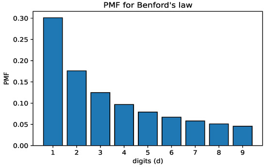
Figure 2.
Probability Measure for Benford’s Law in Base 10.
Benford’s law appears throughout purely mathematical constructions as well as geometric series, recurrence relations, and geometric Brownian motion. Its ubiquity makes it one of the most interesting objects in modern mathematics, as it arises in many disciplines. Therefore, it is worthwhile to consider non-traditional data sets where the law may appear, such as fractal sets. Basic fractals such as the Cantor set and Sierpinski triangle are obtained as the limiting iterations of sets, and as a result, their unique component measures follow a geometric distribution, which is Benford in most bases. Building on these results, it is plausible that more complicated fractals obey this distribution as well. We studied the Riemann mapping of the exterior of the Mandelbrot set to the complement of the unit disk, along with its reciprocal. These mappings are given by a Taylor and Laurent series, respectively, and we studied their coefficients to determine their fit for Benford’s law. These coefficients are of interest as their asymptotic convergence is intimately related to the conjectured local connectivity of the Mandelbrot set, which is an important open problem in complex dynamics.
4.1. Statistical Testing for Benford’S Law
A common statistical methodology for evaluating whether a data set is distributed according to Benford’s law is to utilize the standard goodness of fit test. As we are investigating Benford’s law in base 10, we utilize 8 degrees of freedom for our testing.(There are nine possible first digits, but once we know the proportion that is digits 1 through 8 the percentage that starts with a 9 is forced, and thus we lose one degree of freedom.) If there are N observations, letting be the Benford probability of having a first digit of d, we expect values to have a first digit of d. If we let be the observed number with a first digit of d, the value is
If the data are Benford, with 8 degrees of freedom, then 95% of the time the value will be at most 15.5073; this corresponds to a significance level of . We perform multiple testing by creating a distribtuion of values as a function of the sample size by calculating the values of the first m values in the dataset. This is standard practice for studying Benford sequences, and we conduct this account for periodicity in the values, which is typical for certain Benford data sets, such as the integer powers of 2. To account for this multiplicity, we also incorporate the standard Bonferroni correction so that the overall testing is conducted at the same level of significance while giving equal weight in terms of significance to each individual test. We do this by making each test be completed at a significance level of . In particular, we perform 10,045 tests for the and 10,046 tests for the coefficients as we compute the statistic each time we add a new non-zero coefficient to our data set. This brings our final corrected threshold value to 38.9706 and 38.9708, respectively. This corresponds to = 0.05/10,045 = 4.978 × 10 for each individual hypothesis in the dataset and = 0.05/10,046 = 4.977 × 10 for each individual hypothesis in the dataset.
Each data point is not independent, as the values are computed by using a running total of the data, and as such, each point is built on the previous one. This results in a high correlation between the data, and Bonferroni correction likely overcompensates for the increase in type I error in our multiple testing. Still, it is one of the most plausible methods of dealing with the increase in multiplicity, since it is one of the simplest and most conservative estimates, and a value above the Bonferroni correction provides strong evidence that the data are not Benford. Using independent increments to compute each statistic for Benford’s law would fix the issue of independence, but is not recommended since periodic behavior can be missed if the increments are chosen poorly relative to the frequency in the data, and this has the potential to lead to erroneous conclusions.
Since the data set is built iteratively, we also provide a curve to represent the Bonferroni correction for m tests. The rationale is to keep the significance of the overall test constant with respect to the number of tests performed. As we increase the total number of tests performed, we wish to increase our correction accordingly. As such, it does not make sense to consider every value on our plot of values with the same threshold, and this curve is provided as a reference for the tests performed on subsets of our data.
We considered the distribution of the values to account for random fluctuations and periodic effects. The distribution’s limiting behavior provides our benchmark for the fit to Benford’s law. In addition, we provide the provide the p-value of our computed statistic to provide the type I error rate for our conclusions, and we compute the powers of the tests relative to our null hypothesis that the data are Benford by using the noncentral chi-squared distribution [15]. We also conducted simulations to estimate the sampling error relative to our null hypothesis. We wish to see how likely it is that a random sample falls in the rejection region for our testing; based on our significance level of , we expect the sampling error to be roughly 5% if the data are Benford. We randomly sample 1000 coefficients from our data sets and calculate the value for this sample data. We repeat this simulation 1000 times, and take the ratio of values in the rejection region to the total number of sample statistics calculated, to estimate the sampling error.
An equivalent test is to consider the distribution of the base 10 logarithms for the absolute value of the data set modulo 1; as a necessary and sufficient condition for a Benford distribution, this sequence converges to the uniform distribution [16]. As a measure of quantifying the uniformity of this distribution, we may again consider the standard test. We only perform a single test for the total data set, so we do not need to account for multiplicity. Specifically, we split the interval into 10 equal bins. If the data are uniform, we expect that each bin obtains of the total data. Therefore, for each bin in the data we expect a value of and for each bin in the data we expect a value of . Since there are 10 possible observations, we have 9 degrees of freedom for the data. If the percentage of the data in the first nine bins is known, then the percentage of data in the last bin is forced, and we lose one degree of freedom. We again take and for nine degrees of freedom, this corresponds to a value of 16.919. These results are generated by cells 16, 17, and 18 by the Jupyter notebooks amLogData.ipynb and bmLogData.ipynb, respectively, which may be found under the Data Analysis folder. We also provide the associated p-values and powers of the statistic relative to the null hypothesis that this data are uniform.
The coefficients we studied are 2-adic rational numbers, so we considered the distributions of the numerators, denominators, and decimal expansions separately. We considered only the non-zero coefficients, since zero is not defined for our probability measure, and certain theorems and conjectures outlined by Shiamuchi in [4] already describe the distribution of the zeroes in the coefficients. Our goal is to identify which components of these coefficients are a good fit for Benford’s law through statistical testing, and it is hoped that this will provide motivation for a formal proof.
Table 1 provides examples of the coefficients computed. When the coefficient is 0, numerators are set to 0 and denominators to - for readability. We then use them to compute the exact values in decimal expansion for and .

Table 1.
The table of first 11 coefficients computed.(codes/coeff_compute.py).
4.2. Benfordness of the Taylor and Laurent Coefficients
We examine the distribution of the first digits of the and coefficients. As mentioned earlier, we restrict our discussion to the non-zero coefficients. We conduct the test and distribution of the base 10 logarithms modulo 1 to evaluate the data. The plots of the values are shown in Figure 3, Figure 4 and Figure 5; these figures were generated by cells 16, 17, and 18 in the Jupyter notebooks amChiSquareData.ipynb and bmChiSquareData.ipynb respectively, which may be found under the Data Analysis folder. The plots of the logarithms modulo 1 are provided in Figure 6, Figure 7 and Figure 8; these figures were generated by cells 10,11, and 12 in the Jupyter notebooks amLogData.ipynb and bmLogData.ipynb, respectively, which may be found under the Data Analysis folder. Simulation results can be reproduced using a sampling_simulation.ipynb notebook in the same folder.
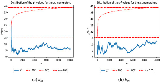
Figure 3.
distribution for the and numerators. Legend Guide: FBC-Final Bonferroni Correction, BCC-Bonferroni Correction Curve.
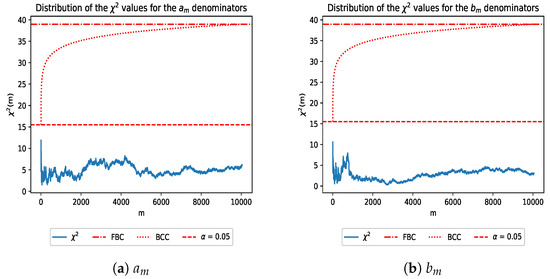
Figure 4.
distribution for the and denominators. Legend Guide: FBC-Final Bonferroni Correction, BCC-Bonferroni Correction Curve.
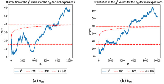
Figure 5.
distribution for the and decimal expansions. Legend Guide: FBC-Final Bonferroni Correction, BCC-Bonferroni Correction Curve.
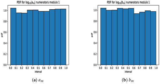
Figure 6.
and numerators.
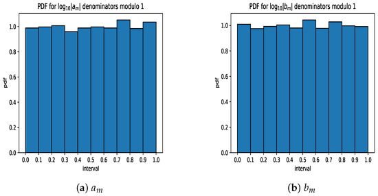
Figure 7.
and denominators.
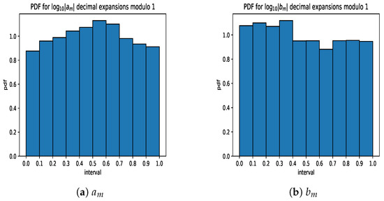
Figure 8.
and decimal expansions.
On the plots of the values, the numerators stay below the uncorrected threshold for statistical significance. The coefficients seem to settle towards the end of the distribution while the coefficients end during a period of relative inflation with many fluctuations. Bearing this in mind, the results for the numerators will be slightly worse than the numerators due to the behavior of the distribution at the point where we finished collecting our data. The final values for the and numerators are 5.968 and 12.785, respectively. The type I error rates (p-values) for the final values are 0.651 and 0.119, both of which are greater than our critical values of for the individual hypotheses and for the overall test. The sampling errors we obtain from our simulations for and are 0.043 and 0.058. The powers relative to the null hypothesis for and are 0.355 and 0.718, respectively. As a result, there is not sufficient evidence to reject our null hypothesis that the data are Benford.
The denominators stay well below the original threshold. This is expected, as they consist of a random sampling of a geometric series, which is known to be Benford in most bases [16]. The final values for the and denominators are 6.148 and 3.093, respectively. The type I error rates (p-values) for the final values are 0.631 and 0.928, both of which are greater than our critical values of for the individual hypotheses and for the overall test. The sampling errors we obtain from our simulations for and are 0.047 and 0.028. The powers relative to the null hypothesis for and are 0.366 and 0.187, respectively. As a result, there is not sufficient evidence to reject our null hypothesis that the data are Benford based on this testing.
The values for the decimal expansions are the most interesting. The values for the coefficients seem to increase in general, but there are erratic periods where the values fall. The sequence ends above the final corrected threshold for significance, and it is plausible that the values will continue to increase more quickly than the correction allows with extra data. The meanwhile surpasses the corrected threshold, which is strong evidence that they are not Benford; the values in the data do decrease towards the end of the distribution, but it is still well above the threshold for significance. The final values for the and data are 58.054 and 51.934, respectively. The type I error rates (p-values) for the final values are × 10 and × 10, both of which are less than our critical values of for the individual hypotheses and for the overall test. The sampling errors we obtain from our simulations for and are 0.235 and 0.243. The powers relative to the null hypothesis for and are 0.999992 and 0.999956, respectively. As a result, there is sufficient evidence to reject our null hypothesis that the data are Benford based on this testing.
As for the distribution of the base 10 logarithms modulo 1, the numerators have a skew towards zero in the distribution of their logarithms. There is a pattern in the coefficients that explains their behavior, we have observed that when , . This result seems to generalize for , such that when , = 1/m, which can be observed in the tables provided by Shiamuchi in [4], and we have not found a counterexample in our computations. There is regularity in the numerators as discussed by Bielefeld, Fisher, and von Haeseler in [11], and it is likely that similar regularities are present in the coefficients as well. It seems that these patterns become less frequent as the sample size increases. The extra regularity in the coefficients also helps explain why their distribution is more skewed towards 0 relative to the one provided for the coefficients as well. Still, for a finite number of iterations, we do not expect perfect agreement, and convergence is likely with larger samples. The values for the and data are 8.482 and 10.203, respectively. These correspond to p-values of 0.486 and 0.334; the powers relative to the null hypothesis are 0.482 and 0.574. There is not sufficient evidence to reject the null hyopthesis that the data are uniform. In turn, this provides further evidence that the data are Benford.
The denominators consist of a sampling of integer powers of 2. Since is irrational, the sequence is Benford in base 10, and (mod 1) converges to the uniform distribution [16]. Since the denominators span many orders of magnitude, it is expected that they will similarly converge in distribution. The values for the and data are 6.334 and 4.416, respectively. These correspond to p-values of 0.706 and 0.882; the powers relative to the null hypothesis are 0.358 and 0.248. There is not sufficient evidence to reject the null hyopthesis that the data are uniform. In turn, this provides further evidence that the data are Benford.
The values for the and decimals are 64.261 and 60.757, respectively. These correspond to p-values of × 10 and × 10; the powers relative to the null hypothesis are 0.99998 and 0.99994. There is sufficient evidence to reject the null hyopthesis that the data are uniform. This provides further evidence that the data are not Benford. It is worth noting that the distribution is skewed towards the second half of the interval, while the distribution is skewed towards the first half of the interval. This asymmetry may be related to how the series represent coefficients of reciprocal functions and how they may be computed from each other.
We may also investigate how many orders of magnitude a data set spans on average by computing the arithmetic mean and standard deviation of to tell where the data set is centered and how spread out it is. It is typical, but not necessary, for a data set to be Benford if it spans many orders of magnitude (see Chapter 2 of [7,17] for an analysis that a sufficiently large spread is not enough to ensure Benfordness). Our findings for the Taylor and Laurent coefficients are summarized in Table 2. The data are generated by cell 8 in the Jupyter notebooks amLogData.ipynb and bmLogData.ipynb, respectively, which may be found under the Data Analysis folder.
Table 2.
Parameters for the distribution of the data sets.
The numerators and denominators span many orders of magnitude, but the decimal expansions cluster. The mean for the decimal expansions being negative indicates that the denominators are larger than the numerators, on average. The ratio between the growth rates of the numerators and denominators likely has some form of regularity as well to account for the small standard deviation, but more analysis would be needed to determine the exact relationship. These observations are consistent with the previously discussed conjecture that for all m, and it is plausible a similar relation holds for the coefficients as well. Ultimately, this provides insight into the growth of the coefficients and the shape of the data, and this motivates our conclusion that the numerators and denominators appear to converge to a Benford distribution, while there is no strong evidence for convergence in the decimal expansions.
5. On the Taylor and Laurent Coefficients
This Section deals with observations and theorems on the coefficients from various authors. Our goal is to compile and highlight important results from disparate sources. We link to the papers where the original observations may be found and their proofs when applicable. Section 5.1 deals specifically with observations related to the coefficients, Section 5.2 deals with the coefficients, and Section 5.3 deals specifically with new observations we make.
Theorem 3 highlights the relevance of the study of the Riemann mappings and . Much effort has been put into the understanding of the behavior of both series. We now refer to a few important results and introduce new conjectures on the behavior of the coefficients. One of the most important theorems relating to both sets of coefficients is the following.
Theorem 7.
The and coefficients are d-adic rational numbers. In other words, and are of the form
where p is an integer indivisible by d. The integer ν is, by definition, the d-adic valuation of or .
This is a combination of Theorems outlined by Shiamuchi in [3,8], and it provided our motivation for studying the numerators, denominators, and decimal expansions, separately. We consider only the case . The majority of the following results hold also for a general integer , under simple modifications.
5.1. Results for the Taylor Coefficients
Remark 3.
For any integers k and ν satisfying and , let . Then
It is unknown whether the converse is true. The proof may be found in [18]. The authors have reported that their computation of 1000 terms of has not produced a zero-coefficient besides those indicated by the theorem, which is consistent with our observations. The result may also be expressed as the following corollary:
Corollary 1.
Let with and odd. If , then .
Making use of the 2-adic valuation, it is possible to obtain the following theorem, as outlined in [4].
Theorem 8.
We have for all m, with equality attained exactly when m is odd.
In the following, since our interest is only for the 2-adic valuation, we will make use of the notation , and we immediately obtain the following remark.
Remark 4.
In the case that m is odd, we may obtain an efficient algorithm to compute through . Following immediately from Theorem 8 by the properties of the d-adic evaluation outlined in [3], we have,
Therefore, if we set a value, N, the denominator’s exponent for every odd number is given by
We may also summarize Theorem 3.1 and Corollary 3.5 from [8] for the case that .
Theorem 9.
Given , we have that , where
Under the same assumptions, the result is also true with
5.2. Results for the Laurent Coefficients
Similar results hold for the coefficients. We use the notation , where is odd. The first result was presented in [19] in 1988.
Remark 5.
If and , then .
It is still unknown whether the converse of this theorem is true. In [5], the only coefficients that have been observed to be zero are those mentioned in this theorem. The following result, from [11], underlines that a result similar to the one for the holds.
Theorem 10.
We have for all m, and equality is attained exactly when m is odd.
Don Zagier has made several observations and conjectures about the exponents of . We shall later extend them to the coefficients. The original conjectures are outlined in [11].
Conjecture 1.
For thecoefficients, we have the following.
- If, then.
- If, then, whereifmod 12 and 1 otherwise.
- If, then, wheremoves with periodicity of 28, as expressed in [11].
5.3. New Remarks on the Coefficients
Remark 6.
Theorem 10 and the results on reported in Remark 4 imply that the denominator’s coefficients for have regularity in terms of consecutive differences for odd m. Zagier’s conjectures posit similar patterns for even m. This gives a constant discrete derivative in the denominator’s exponents for , , . Note that for each of these subsequences, there are some starting values of 0. These correspond exactly with the values predicted by Corollaries 1 and 5, respectively; when , the algorithm gives 0 for the denominator’s exponent. In general, for each n there is a partial periodicity with period in , and equivalently, in m.
Another direction is to calculate the slope of each of the subsequences, since they seem to grow linearly. Our observations make use of the previous remark and have led to the following conjecture.
Conjecture 2.
Conjecture 1 Let m be written as as before, with fixed. Then, the sequence is asymptotically linear, with slope
The numerators tend to follow similar behavior as the denominators. In particular, the modulus of the numerators in the subsequences tend to organize as follows: > > ⋯. The possibility of bounding the numerators by making use of its associated denominator is a subject of further study.
We now extend Conjecture Section 5.2 to the coefficients, as follows:
Conjecture 3.
For the coefficients we have:
- If, , and
-
Table 3. The distribution of when has periodicity 16 × 12. From , it repeats itself, and will have the same () of and following.
This suggests a partial periodicity with period in , or of in m. As before, it is possible to write as , but it is more difficult to identify a general pattern in this case.
6. Future Work
The most natural extension of our work would be to generate more coefficients, which would allow more thorough statistical testing. Given more data, we could look at the coefficients over a certain zoom or average the coefficients over certain subsets. It would be particularly interesting if certain subsets of the coefficients also converge to the Benford distribution. We may also look at the powers of the denominators to observe whether they follow a Benford distribution.
The algorithms for computing the coefficients of the Mandelbrot can also be easily generalized to obtain other abstract Multibrot sets, which could be analyzed using the same methods. We could look at the data in different bases to observe whether Benfordness holds there. It would be interesting to se the numerators and decimal expansions of the coefficients for the Multibrot set of degree d follow a Benford distribution in base d while it is trivial to observe that the denominators will not.
The results of Section 5 also present interesting extensions for future work. In particular, Remark 6 suggests that dividing the coefficients into subsequences to be bounded separately may be the best approach to study the convergence of the Laurent series of the coefficients. This approach, which has not been followed in the past, to the best of our knowledge, could provide valuable results in the study of the local connectedness of .
Author Contributions
This paper is a result of a collaborative effort of all the authors on all aspects of the work, with J.D. on visualization and formal analysis, W.F. on data curation and software, and F.B. on formal analysis and conceptualization. The research was performed as part of the 2021 Polymath Jr program, advised by T.C.M., S.J.M. and D.S. All authors have read and agreed to the published version of the manuscript.
Funding
This work was partially supported by NSF Grant DMS2113535.
Institutional Review Board Statement
Not applicable.
Informed Consent Statement
Not applicable.
Data Availability Statement
The codes and data can be found here https://github.com/DannyStoll1/polymath-fractal-geometry (accessed on 2 July 2022).
Acknowledgments
We thank our colleagues from the 2021 Polymath Jr REU program for helpful comments on earlier drafts.
Conflicts of Interest
The authors declare no conflict of interest.
References
- Douady, A.; Hubbard, J. Exploring the Mandelbrot set. Publ. Math. Orsay 1985. Available online: https://pi.math.cornell.edu/~hubbard/OrsayEnglish.pdf (accessed on 2 July 2022).
- Luo, J.; Yao, X. To Generalize Carathéodory’s Continuity Theorem. arXiv 2020, arXiv:2002.08644. [Google Scholar]
- Shiamuchi, H. A remark on Zagier’s observation of the Mandelbrot set. Osaka J. Math. 2015, 52, 737–747. [Google Scholar]
- Shiamuchi, H. On the coefficients of the Riemann mapping function for the exterior of the Mandelbrot set. RIMS KôKyûRoku Bessatsu 2012, 1807, 21–30. [Google Scholar]
- Ewing, J.H.; Schober, G. The area of the Mandelbrot set. Numer. Math. 1992, 61, 59–72. [Google Scholar] [CrossRef]
- Benford, F. The Law of Anomalous Numbers. Proc. Am. Philos. Soc. 1938, 78, 551–572. [Google Scholar]
- Miller, S.J. Theory and Applications of Benford’s Lawn; Princeton University Press: Princeton, NJ, USA, 2015. [Google Scholar]
- Shiamuchi, H. Taylor Coefficients of the Conformal Map for the Exterior of the Reciprocal of the Multibrot Set. Interdiscip. Inf. Sci. 2019, 25, 33–44. [Google Scholar] [CrossRef]
- Milnor, J. Dynamics in One Complex Variable, 3th ed; Princeton University Press: Princeton, NJ, USA, 2011. [Google Scholar]
- Stoll, D. A Brief Introduction to Complex Dynamics; University of Chicago: Chicago, IL, USA, 2015; pp. 1–23. [Google Scholar]
- Bielefeld, B.; Fisher, Y.; von Haeseler, Y. Computing the Laurent Series of the Map Ψ: C\D¯ → C\M. Adv. Appl. Math. 1993, 14, 25–38. [Google Scholar] [CrossRef][Green Version]
- Bandt, C.; Keller, K. Symbolic dynamics for angle-doubling on the circle. II. Symbolic description of the abstract Mandelbrot set. Nonlinearity 1993, 6, 377–392. [Google Scholar] [CrossRef]
- Benini, A.M. A survey on MLC, Rigidity and related topics. arXiv 2018, arXiv:1709.09869. [Google Scholar]
- Shiamuchi, H. On the coefficients of the Riemann mapping function for the complement of the Mandelbrot set. RIMS Kôkyûroku Bessatsu 2011, 1772, 109–113. [Google Scholar]
- Guenther, W.C. Power and Sample Size for Approximate Chi-Square Tests. Am. Stat. 1977, 31, 83–85. [Google Scholar]
- Miller, S.J.; Takloo-Bighash, R. An Invitation to Modern Number Theory; Princeton University Press: Princeton: NJ, USA, 2006. [Google Scholar]
- Berger, A.; Hill, T.P. Benford’s law strikes back: No simple explanation in sight for mathematical gem. Math. Intell. 2011, 33, 21–30. [Google Scholar] [CrossRef]
- Ewing, J.H.; Schober, G. Coefficients associated with the reciprocal of the Mandelbrot Set. J. Math. Anal. Appl. 1992, 1, 104–114. [Google Scholar] [CrossRef]
- Levin, G.M. On the arithmetic properties of a certain sequence of polynomials. Commun. Mosc. Math. Soc. 1988, 43, 245–246. [Google Scholar] [CrossRef]


Publisher’s Note: MDPI stays neutral with regard to jurisdictional claims in published maps and institutional affiliations. |
© 2022 by the authors. Licensee MDPI, Basel, Switzerland. This article is an open access article distributed under the terms and conditions of the Creative Commons Attribution (CC BY) license (https://creativecommons.org/licenses/by/4.0/).