An Adaptive Generalized Cauchy Model for Remaining Useful Life Prediction of Wind Turbine Gearboxes with Long-Range Dependence

Abstract

Remaining useful life (RUL) prediction is important for wind turbine operation and maintenance. The degradation process of gearboxes in wind turbines is a slowly and randomly changing process with long-range dependence (LRD). The degradation trend of the gearbox is constantly changing, and a single drift coefficient is not accurate enough to describe the degradation trend. This paper proposes an original adaptive generalized Cauchy (GC) model with LRD and randomness to predict the RUL of wind turbine gearboxes. The LRD is explained jointly by the fractal dimension and the Hurst exponent, and the randomness is explained by the diffusion term driven by the GC difference time sequence. The estimated value of the unknown parameter of adaptive GC model is deduced, and the specific expression of the RUL estimation is deduced. The adaptability is manifested in the time-varying drift coefficient of the GC model: by continuously updating the drift coefficient to adapt to the change in the degradation trend, the adaptive GC model offers high accuracy in the prediction of the degradation trend. The performance of the proposed model is analyzed using real wind turbine gearbox data.

1. Introduction

As wind energy continues to grow, ensuring the reliability and reducing maintenance of wind turbines gains increasing importance [1,2]. Monitoring the health state and predicting the RUL of wind turbines has become important to limiting premature failures of wind turbines [3,4]. Bearings and gearbox failures are common wind turbines failures [5]. According to the statistics of the latest reliability database in 2011, approximately 76% of wind turbine failures occur due to bearings and gearboxes [6]. Most gearbox failures start at the bearing location and transfer to the gear teeth in the form of bearing fragments leading to shutdown [7,8].

Research has been conducted in wind turbine condition monitoring, fault detection and diagnosis, and failure prediction. The methods proposed are mainly divided into data-driven methods and model-based methods [9]. For example, a multi-class support vector machine is proposed for fault detection and identification in wind power transmission gearboxes by fusing different time-domain and frequency-domain features. An integral extension load mean decomposition multi-scale entropy method is used in [10] to extract features, and a least square support vector machine is developed to perform fault diagnosis and RUL prediction for wind turbines. In [11], an adaptive Bayesian algorithm is used to predict the bearing’s RUL in wind turbines. A practical disadvantage of the data-driven methods is that they usually require historical data of degradation to train the model [12]. Wind turbines are usually complex, large-scale and highly reliable, and obtaining large amounts of fault measurement data is expensive and time-consuming. The degradation process of wind turbine bearings and gearboxes can be affected by many factors (for example, different environmental factors, failure modes, operating conditions, etc.), which introduces difficulties to the construction and training of data-driven models [13]. Therefore, fault diagnosis and failure prediction based on limited fault data samples are still challenging problems [3].

As a practical alternative, model-based wind turbine life prediction methods have been considered. For instance, a gamma model has been proposed in [14] to describe degradation processes. The model parameters are estimated and updated by the maximum likelihood estimation method and Bayesian method, respectively. A monotonic degradation model based on the inverse Gaussian process is used in [15] to describe the degradation process. The change point of the bearing degradation process is considered in [16] to establish a stochastic prediction model based on the Wiener process. However, the degradation of wind turbine gearboxes is a slow and continuous process with the LRD characteristic, which is affected by the historical state evolution. The above-mentioned model-based prediction methods of wind turbine do not take the LRD into account and do not consider the adaptive nature of the drift coefficient.

In this context, the work presented in this paper proposes an adaptive GC model to describe the LRD and randomness of wind turbine degradation. The adaptive GC model considers the time-varying nature of the drift coefficient of the degradation process [17]. In the continuous change in the degradation trend, the drift coefficient is automatically updated and adjusted in real time to adapt to the change so that the adaptive GC model can predict the degradation trend with high accuracy. The LRD and randomness are explained by the diffusion term driven by the GC difference time sequence. The LRD of the GC process is evaluated by its autocorrelation function (ACF) [18]. The GC process is considered to satisfy the LRD characteristics if its ACF integral diverges. Based on the integration of ACF, the GC process has been found to satisfy the LRD characteristic when $0<(4-2D)(2-2H)\le 1$ [19]. H is the Hurst index, and D is the fractal dimension. The GC process satisfies the LRD characteristics, which means that its ACF slowly decays to the extent of integral divergence. According to the above conditions, the LRD characteristics of the GC process are jointly evaluated by the fractal dimension and the Hurst exponent.

In summary, the main contributions of this paper are highlighted as follows:

• The LRD prediction model driven by a GC process is introduced to describe the degradation process of wind turbine gearboxes. The LRD is explained jointly by the fractal dimension and the Hurst exponent, and the randomness is explained by the diffusion term driven by the GC difference time sequence;
• The time-varying drift coefficient is used to describe the adaptive update of the degradation trend, and the parameter estimation and RUL estimation of the adaptive GC model are deduced;
• The normality test of the GC difference time sequence ensures the accuracy of the multi-dimensional joint distribution of the predicting model.

The remaining sections of this paper are organized as follows. Section 2 describes the LRD characteristics of the GC process. The GC difference time sequence is constructed by ACF, and a normality test is carried out. Section 3 proposes an adaptive GC model and derives the parameter estimation and RUL estimation of the degradation model. Section 4 describes how the proposed procedure is applied to online monitoring and RUL prediction of wind turbines gearboxes. Finally, Section 5 is the conclusion of this paper.

2. Properties of the GC Process and Its Simulation

2.1. The LRD Characteristic of The GC Process

Let $\{x(t),0<t<\infty \}$ be a GC stochastic process; the ACF, $R(\tau )$, of $x(t)$ can be written as follows [19]:

$$R(\tau )=E[x(t+\tau )x(t)]={(1+{\tau }^{\alpha })}^{-\beta /\alpha },$$

(1)

where $\tau$ is the lag time, and $\alpha$ and $\beta$ are parameters describing the LRD characteristics. The LRD characteristics of the GC process are evaluated jointly by the Hurst index $H$ and the fractal dimension $D$, which represent global self-similarity and local roughness, respectively. The specific relationships are $H=1-\beta /2,D=2-\alpha /2$ [19].

If the improper integral of the ACF of $x(t)$ on $(0,\infty )$ is infinite, then $x(t)$ is said to be a stochastic process with LRD characteristics. The infinite integration of the ACF can be calculated as follows:

$${\mathrm{\int }}_0^{+\infty }R(\tau )d\tau ={\mathrm{\int }}_0^{+\infty }{(1+{\tau }^{\alpha })}^{-\beta /\alpha }d\tau =\left\{\begin{array}{c}\frac{1}{\alpha }B(\frac{1}{\alpha },\beta -\frac{1}{\alpha }),\begin{array}{cc}& if(\alpha \beta >1)\end{array}\\ \infty ,\begin{array}{cc}& if(0<\alpha \beta <1)\end{array}\end{array}\right.,$$

(2)

where $B(x,y)=\Gamma (x)\Gamma (y)/\Gamma (x+y)$ is the beta function and $\Gamma (·)$ is the gamma function. Consider the condition when $\alpha \beta =1$,

$${\mathrm{\int }}_0^{+\infty }R(\tau )d\tau ={\mathrm{\int }}_0^{+\infty }{(1+{\tau }^{\alpha })}^{-1/{\alpha }^2}d\tau =\frac{B(1/\alpha ,0)}{\alpha }=\frac{\Gamma (1/\alpha )\Gamma (0)}{\alpha \Gamma (1/\alpha )}=\frac{\Gamma (0)}{\alpha },$$

(3)

which diverges since $\Gamma (z)\sim 1/z$ as $z\to 0$. Thus,$\Gamma (0)/\alpha \sim \infty$ and the GC process is LRD for $0<\alpha \beta \le 1$, whereas it is short-range dependent if $\alpha \beta >1$. According to the definition of LRD, we obtain that when $0<\alpha \beta \le 1$, the GC process satisfies the LRD condition:

$${\mathrm{\int }}_0^{+\infty }R(\tau )d\tau =\infty , if(0<\alpha \beta \le 1).$$

(4)

Substituting the fractal dimension and Hurst exponent for $\alpha$ and $\beta$, one obtains the evaluation criterion for LRD, $0<(4-2D)(2-2H)\le 1$. The ACF for different values of $H$ and $D$ is plotted in Figure 1.

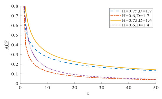
Figure 1. The ACF of the GC process.

It can be seen from Figure 1 that low $D$ and high $H$ values make the ACF curve decay slowly. When the lag time is large enough, the ACF curve does not decay to zero and the improper integral in Equation (4) diverges.

2.2. The Construction of the GC Difference Time Sequence

In this paper, the ACF is used to construct the GC time sequence. The specific steps are as follows.

Step 1: The power spectral density (PSD) function of the GC process is obtained from the relationship between the ACF and the PSD:

$$S(\omega )=F[R(\tau )]=F\left[{(1+{\left|\tau \right|}^{\alpha })}^{-\beta /\alpha }\right],$$

(5)

where $F$ stands for the Fourier transform. Suppose that $H(\omega )$ and $h(t)$ are the system function and impulse response function, respectively, and that $h(t)$ is the inverse Fourier transform of $H(\omega )$. The relationship between the power spectral density function $S(\omega )$ and the system function $H(\omega )$ is $S(\omega )={\left|H(\omega )\right|}^2$. From Equation (5), we can derive the expression of the impulse response function $h(t)$:

$$h(t)=F^{-1}[\sqrt{S(\omega )}]=F^{-1}\left\{F{\left[{\left(1+{\left|\tau \right|}^{4-2D}\right)}^{-\frac{1-H}{2-D}}\right]}^{0.5}\right\}.$$

(6)

Step 2: The GC time sequence can be obtained from the white noise signal and the impulse response function of the GC process [20]:

$$y(t)=w(t)\ast h(t)=w(t)\ast F^{-1}\left\{F{\left[{\left(1+{\left|\tau \right|}^{4-2D}\right)}^{-\frac{1-H}{2-D}}\right]}^{0.5}\right\},$$

(7)

where $w(t)$ is the white noise signal. Suppose that the frequency spectrum of unit white noise is $W(\omega )=\exp (j\theta (\omega ))$. The white noise signal $w(t)$ is obtained by inverse Fourier transform of the frequency spectrum $W(\omega )$ of the white noise:

$$w(t)=F^{-1}\left[W(\omega )\right]=\frac{1}{2\pi }{\mathrm{\int }}_{-{\omega }_c}^{{\omega }_c}\exp (j\theta (\omega ))\exp (j\theta (\omega ))d\omega .$$

(8)

Step 3: Set the time interval to 1 and obtain the GC difference time sequence through the difference $dGC(t)=GC(t+1)-GC(t)$.

The specific flowchart of the above generation procedure is shown in Figure 2.

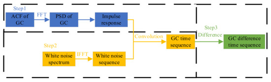
Figure 2. Flowchart of the procedure for generating the difference time sequence.

The GC time sequence is generated with $D=1.2$ and $H=0.7$. The GC difference time sequence is shown in Figure 3.

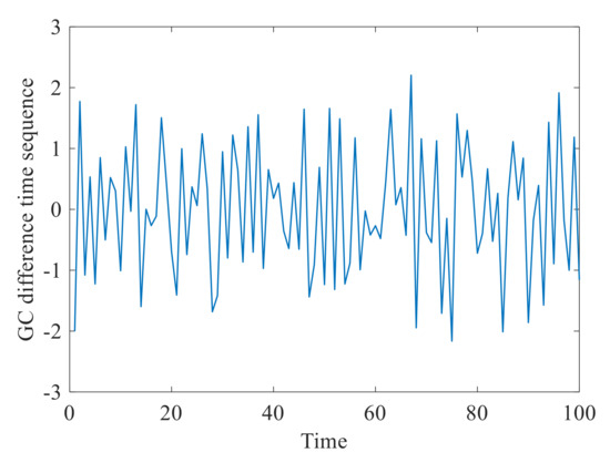
Figure 3. GC difference time sequence.

2.3. The Normality Test on the GC Difference Time Sequence

The PSD is generated by the Fourier transform of the ACF of the GC process, and the impulse response function is obtained by the system function. Then, the GC time sequence is obtained by convolving the impulse response function with the white noise sequence. Finally, the first-order difference processing is performed to obtain the GC difference time sequence. Before obtaining the distribution to which the increment of the degradation process obeys, it is necessary to test the normality of the GC difference time sequence. The histograms under different lengths of the GC difference time sequence are shown in Figure 4. The histogram test, the joint test of skewness and kurtosis, the Shapiro–Wilk (SW) test and the Kolmogorov–Smirnov (KS) test were used to verify the normality of the GC difference time sequence [21,22].

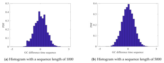
Figure 4. The histograms of GC difference time sequence.

It can be seen from Figure 4 that as the length of the time sequence increases, the time sequence is closer to the normal distribution. The skewness describes the symmetry of the time sequence, and the skewness of the normal distribution is zero. The kurtosis describes the steepness of the time sequence, and the kurtosis of the normal distribution is three. The result of the joint test of skewness and kurtosis is shown in Table 1.

Table 1. The Joint Test of Skewness and Kurtosis of GC Difference Time Sequence.

Length of Time Sequence	100	500	1000	2000	5000
mean value of skewness	−0.1291	0.1067	0.0672	0.0867	−0.0498
mean value of kurtosis	2.8574	3.0816	2.9410	3.0737	2.9841

In Table 1, skewness and kurtosis are close to zero and three, respectively, under different sequence lengths. The results of the SW test and KS test are shown in Table 2 and Table 3, respectively.

Table 2. The SW Test on the C Difference Time Sequence.

Length of Time Sequence	100	500	1000	2000	5000
Statistics	0.980	0.997	0.998	0.999	1.000
p-values	0.131	0.527	0.738	0.827	0.919

Table 3. The KS Test on the GC Difference Time Sequence.

Length of Time Sequence	100	500	1000	2000	5000
Statistics	0.833	0.683	0.520	0.516	0.498
p-value	0.491	0.739	0.950	0.953	0.965

In Table 2 and Table 3, the p-values of the different-length time sequences after the SW test and the KS test are larger than 0.05, which shows that there is no significant difference between the GC difference time sequence and the normal distribution. Therefore, the GC difference time sequence obeys the normal distribution.

3. Degradation Modeling and RUL Prediction Based on Adaptive GC Model

3.1. The Adaptive GC Model

The degradation process of wind turbine gearboxes can be described as [23]

$$d{y}_k=a_k{\Lambda }_k(t_k)+\sigma dB(t_k),$$

(9)

where $y_k$ is the degradation value at time $t_k$,$d{y}_k$ is the difference of $y_k$,$a_k{\Lambda }_k$ is the drift function of the degradation process, reflecting the degradation trend item ${\Lambda }_k$ is a function of time $t_k$ and $\sigma dB(t_k)$ is the diffusion function of the degradation process.

The GC degradation process is obtained by replacing the random term $B(t_k)$ with $GC(t_k)$ [24]:

$$d{y}_k=a_k{\Lambda }_k+\sigma dGC(t_k).$$

(10)

In order to express the time-varying nature of the degradation trend, suppose that $a=[a_1,a_2,\dots ,a_n]$ is a time-varying drift coefficient that obeys the normal distribution $N({\mu }_a,{\sigma }_a^2)$. Then, an adaptive GC model is proposed. Adaptability is necessary to automatically adjust and update the model parameter values and associated RUL expressions according to the data characteristics. The principle of adaptive update of the drift coefficient is shown in Figure 5. The cycle ends when the health indicator (HI) exceeds the fault threshold (FT). Bringing the difference time sequence into Equation (10) yields Equation (11):

$$d{y}_k=a_k{\Lambda }_k+\sigma [GC(t_k+1)-GC(t_k)].$$

(11)

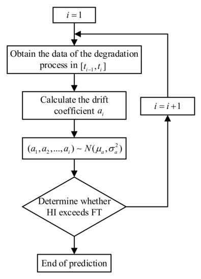
Figure 5. Adaptive update of the drift coefficient.

3.2. Parameter Estimation in the Adaptive GC Model

There are five unknown parameters—${\mu }_a,{\sigma }_a,\sigma ,H,D$—in Equation (11), the values of which need to be determined. Let us denote the unknown parameter vector as $\Phi =[{\mu }_a,{\sigma }_a,\sigma ,H,D{]}^T$, where ${[·]}^T$ represents the transpose of the vector. The maximum likelihood estimation method is used to estimate the values of the unknown parameters based on actual degradation data. Suppose that the measured values of the degradation process of the HI at time $t_1,t_2,\dots ,t_n$ are contained in the vector variable $Y={[y_1,y_2,\dots ,y_n]}^T$, where $n$ is the number of measurements. Let $\Lambda =[{\Lambda }_1,{\Lambda }_2,\dots ,{\Lambda }_n{]}^T$. According to the nature of the independent increment of the GC process, the multi-dimensional random variable $Y$ follows:

$$Y\sim N({\mu }_a,\Lambda ,{\sigma }_a^2,{\sigma }^2,Q),$$

(12)

where $Q$ is the covariance matrix of the GC process. The likelihood function is obtained from the probability density function of the multi-dimensional joint normal distribution

$$l(\Phi |Y)=-\frac{n\ln (2\pi )}{2}-\frac{\ln \left|\Sigma \right|}{2}-\frac{1}{2}(Y-{\mu }_a\Lambda {)}^{\prime }{\Sigma }^{-1}(Y-{\mu }_a\Lambda ),$$

(13)

with

$$\left|\Sigma \right|=\left|{\sigma }^{2}Q\right|(1+{\sigma }_a^2{\Lambda }^{\prime }{({\sigma }^{2}Q)}^{-1}\Lambda ),$$

(14)

$${\Sigma }^{-1}={({\sigma }^{2}Q)}^{-1}-\frac{{\sigma }_a^2{({\sigma }^{2}Q)}^{-1}\Lambda {\Lambda }^{\prime }{({\sigma }^{2}Q)}^{-1}}{1+{\sigma }_a^2{\Lambda }^{\prime }{({\sigma }^{2}Q)}^{-1}\Lambda }.$$

(15)

Calculating the partial derivatives of Equation (13) can predict the parameters ${\mu }_a$ and ${\sigma }_a$, respectively,

$$\frac{\partial l}{\partial {\mu }_a}={\Lambda }^T\Sigma Y-{\mu }_a{\Lambda }^T{\Sigma }^{-1}\Lambda ,$$

(16)

$$\frac{\partial l}{\partial {\sigma }_a^2}=-\frac{{\Lambda }^T{({\sigma }^{2}Q)}^{-1}\Lambda }{2(1+{\sigma }_a^2{\Lambda }^T{({\sigma }^{2}Q)}^{-1}\Lambda )}+\frac{{(Y-{\mu }_a\Lambda )}^T{({\sigma }^{2}Q)}^{-1}\Lambda {\Lambda }^{\prime }{({\sigma }^{2}Q)}^{-1}(Y-{\mu }_a\Lambda )}{2{(1+{\sigma }_a^2{\Lambda }^T{({\sigma }^{2}Q)}^{-1}\Lambda )}^2}.$$

(17)

Setting Equations (16) and (17) to 0 and solving to obtain the maximum likelihood estimates of ${\widehat{\mu }}_a$ and ${\widehat{\sigma }}_a^2$

$${\widehat{\mu }}_a=\frac{{\Lambda }^T{\Sigma }^{-1}Y}{{\Lambda }^T{\Sigma }^{-1}\Lambda },$$

(18)

$${\widehat{\sigma }}_a^2=\frac{{(Y-{\mu }_a\Lambda )}^T{({\sigma }^{2}Q)}^{-1}\Lambda {\Lambda }^{\prime }{({\sigma }^{2}Q)}^{-1}(Y-{\mu }_a\Lambda )}{{({\Lambda }^T{({\sigma }^{2}Q)}^{-1}\Lambda )}^2}-\frac{1}{{\Lambda }^T{({\sigma }^{2}Q)}^{-1}\Lambda }.$$

(19)

The contour log-likelihood function about $\sigma$ can be obtained by substituting Equations (18) and (19) into Equation (13):

$$l(\Phi |Y,{\mu }_a={\widehat{\mu }}_a,{\sigma }_a^2={\widehat{\sigma }}_a^2)=-\frac{n\ln (2\pi )}{2}-\frac{\ln \left|\widehat{\Sigma }\right|}{2}-\frac{1}{2}{(Y-{\widehat{\mu }}_a\Lambda )}^T{\widehat{\Sigma }}^{-1}(Y-{\widehat{\mu }}_a\Lambda ),$$

(20)

where $\widehat{\Sigma }={\widehat{\sigma }}_a^2\Lambda {\Lambda }^{\prime }+{\sigma }^{2}Q$. The maximum likelihood value ${\widehat{\sigma }}^2$ can be obtained by maximizing the contour log-likelihood function.

In order to maximize the contour log-likelihood function, it is usually necessary to set the initial value of ${\sigma }^2$. An inaccurate setting of the initial value will affect the result of the estimated values ${\widehat{\sigma }}^2$. The initial values of ${\sigma }^2$ can be obtained as follows:

• Maximize $l(a_1,a_2,\dots ,a_n|Y)$ to obtain the initial estimated values of $a_1,a_2,\dots ,a_n$; the estimated values of $a_1,a_2,\dots ,a_n$ can be obtained by the least square method

  $$l(a_1,a_2,\dots ,a_n|Y)={\displaystyle \sum _{i=1}^n{(Y-a_i\Lambda )}^T(Y-a_i\Lambda )}.$$

  (21)
• Regarding the initial values of $a_1,a_2,\dots ,a_n$ as $n$ actual values of $a_i\sim N({\mu }_a,{\sigma }_a^2)$, the initial estimated values of ${\mu }_a,{\sigma }_a^2$ are obtained by calculating the mean and variance of $a_1,a_2,\dots ,a_n$.
• According to $a_1,a_2,\dots ,a_n$, maximize $l({\sigma }^2|Y)$ to obtain the estimated value ${\widehat{\sigma }}^2$

  $$l({\sigma }^2|Y)=-\frac{n\ln (2\pi )}{2}-\frac{\ln \left|\Sigma \right|}{2}-\frac{1}{2}{(Y-{\mu }_a\Lambda )}^T{\Sigma }^{-1}(Y-{\mu }_a\Lambda ).$$

  (22)

The Hurst exponent $H$ is calculated by the rescaled range (RS) method [25]:

$$R/S=\frac{\underset{1\le i\le N}{\max }{y}_{i,N}-\underset{1\le i\le N}{\min }{y}_{i,N}}{\sqrt{\frac{1}{N-1}{\displaystyle {\sum }_{i=1}^N{(y_i-⟨y⟩)}^2}}},$$

(23)

where $⟨y⟩$ is the mean of the HI, $y_i$ and $y_{i,N}$ are dispersion values, $R$ and $S$ are the range and standard deviation, respectively. The estimated value of the Hurst exponent $H$ is obtained by the logarithmic relationship between $R/S$ and $N$:

$$\ln R/S=H\ln N+b$$

(24)

The value of the fractal dimension $D$ is estimated by the box dimension method [26]:

$$D=\underset{d\to 0}{\lim }\frac{\ln (N_d)}{\ln (1/d)},$$

(25)

where $N_d$ is the total number of squares occupied by the HI and $d$ is the square side length.

3.3. RUL Estimation Based on the Adaptive GC Model

According to the concept of a RUL based on the first arrival time of degradation process to a given failure threshold, RUL at the moment $l_k$ is defined as:

$$L_k=\inf \{l_k:y(l_k+t_k)\ge \omega |y(t_k)<\omega \},$$

(26)

where $\omega$ is the FT. When the gearbox degradation process exceeds FT after the prediction start time (PST) for the first time, it is considered that a fault has occurred, and this time is called the end of life (EOL). In Figure 6, the RUL prediction schematic is clearly explained.

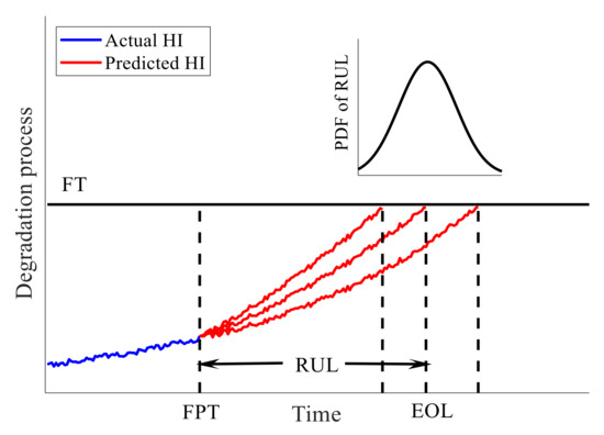
Figure 6. RUL prediction schematic.

Based on the RUL of the Wiener process degradation model, it is easy to obtain the RUL based on the GC process degradation model [27].

$$f_{L_k}(t|y(t_k),\Phi )\cong \frac{\omega -a_k{\Lambda }_k+t{a}_{k}d{\Lambda }_k/dt}{t\sigma \sqrt{2\pi t}}\exp \{-\frac{{(\omega -a_k{\Lambda }_k)}^2}{2t{\sigma }^2}\}.$$

(27)

With the above parameter update mechanism, one can adaptively update the drift coefficient $a_k$ according to the observation data at the current moment. It can be seen from Equation (27) that the expression of the RUL is related to the drift coefficient $a_k$. Next, we discuss the adaptive update of the RUL. The probability density function (PDF) of the RUL is obtained from the total probability formula

$$f_{L_k}(t|y(t_k))=\mathrm{\int }{f}_{L_k}(t|y(t_k),a_k)f(a_k|y(t_k))d{a}_k,$$

(28)

where $f_{L_k}(t|y(t_k))$ is the PDF of the RUL considering the adaptive update of the drift coefficient $a_k$, $f_{L_k}(t|y(t_k),a_k)$ is the conditional PDF of the RUL when the drift coefficient $a_k$ is determined, and $f(a_k|y(t_k))$ is the PDF of the drift coefficient $a_k$ following a normal distribution. If $Z\sim N({\mu }_Z,{\sigma }_Z^2)$, we obtain

$$\begin{array}{l}{E}_Z((K-Z)\exp (-\frac{{(K_1-K_{2}Z)}^2}{2K_3}))\\ =K{E}_Z(\exp (-\frac{{(K_1-K_{2}Z)}^2}{2K_3}))-E_Z(Z\exp (-\frac{{(K_1-K_{2}Z)}^2}{2K_3}))\\ =(K-\frac{{({\sigma }_Z)}^2{K}_1{K}_2+{\mu }_Z{K}_3}{{(K_2{\sigma }_Z)}^2+K_3})\sqrt{\frac{K_3}{{(K_2{\sigma }_Z)}^2+K_3}}\exp (-\frac{{(K_1-K_2{\mu }_Z)}^2}{2({(K_2{\sigma }_Z)}^2+K_3)}).\end{array}$$

(29)

According to the equation for the calculation of the mean value, we can regard $f_{L_k}(t|y(t_k),a_k)$ as the integrand function. Then, Equation (28) can be written as

$$\begin{array}{l}{f}_{L_k}(t|y(t_k))=E_{a_k|y(t_k)}[f_{L_k}(t|a_k,y(t_k))]\\ =\frac{1}{t\sigma \sqrt{2\pi t}}{E}_{a_k}\{(\omega -a_k{\Lambda }_k+t{a}_{k}d{\Lambda }_k/dt)\exp [-\frac{{(\omega -a_k{\Lambda }_k)}^2}{2t{\sigma }^2}\left]\right\}\\ =\frac{{\Lambda }_k-td{\Lambda }_k/dt}{t\sigma \sqrt{2\pi t}}{E}_{a_k}\{(\frac{\omega }{{\Lambda }_k-td{\Lambda }_k/dt}-a_k)\exp [-\frac{{(\omega -a_k{\Lambda }_k)}^2}{2t{\sigma }^2}\left]\right\}.\end{array}$$

(30)

Comparing Equations (29) and (30), we can set $Z$, $K$, $K{ }_1$, $K{ }_2$ and $K{ }_{ 3}$ to $Z=a_k$, $K=\frac{\omega }{{\Lambda }_k-td{\Lambda }_k/dt}$, $K_1=\omega$, $K_2={\Lambda }_k$ and $K_3=t{\sigma }^2$, respectively,

$$f_{L_k}(t|y(t_k))=\frac{\omega S_k-({\Lambda }_k-td{\Lambda }_k/dt)({\sigma }_a^2\omega {\Lambda }_k+{\mu }_{a}t{\sigma }^2)}{t{S}_k\sqrt{2\pi S_k}}\exp [-\frac{{(\omega -{\mu }_a{\Lambda }_k)}^2}{2S_k}],$$

(31)

where $S_k={\Lambda }_k^2{\sigma }_a^2+t{\sigma }^2$. When the drift coefficient $a_k$ updates adaptively, the mean ${\mu }_a$ and variance ${\sigma }_a$ of the drift coefficient $a_k$ also change accordingly. It can be seen from Equation (31) that the PDF of the RUL is related to ${\mu }_a$ and ${\sigma }_a$, so that the RUL is also updated adaptively with the drift coefficient $a_k$. According to the above, the flowchart of the specific procedure for RUL prediction is shown in Figure 7.

Figure 7. Flowchart of the procedure for RUL prediction.

4. Case Study

4.1. Data Description

We consider a case study that concerns experimental data obtained from the FZG test bench of the company STRAM, which operates a wind turbine. As shown in Figure 8, the test bench is composed of a cooling and lubricating controller, gear platform, torque controller and actual operation platform. The sampling frequency is set to 50,000 Hz, and the sampling duration is set to the first 20 s of each minute, that is, one million data are sampled each time. The experimental temperature is set to 70 °C. The vibration signal is collected by an accelerometer placed on the experimental gearboxes. When the amplitude of the collected vibration signal exceeds a certain fault threshold, the experiment stops.

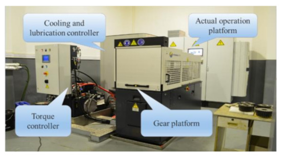
Figure 8. The test bench of gearbox fatigue testing.

In Figure 9, the normal gears before the experiment and the broken gears after the experiment are shown. In this paper, the gearbox vibration signal data collected by the gear contact fatigue test bench are used to verify the effectiveness of the adaptive GC model.

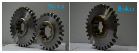
Figure 9. The normal gears and the broken gears.

4.2. Data Preprocessing

In Figure 10, the original signal is depicted, and feature extraction is required to reflect the degradation information of the gearboxes. The unit of sampling interval in Figure 10 is minutes. In Figure 11, nine time-domain features of the data are extracted to describe the degradation process of the gearboxes [28].

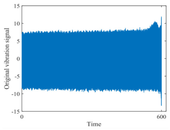
Figure 10. Original vibration signal of the gearboxes.

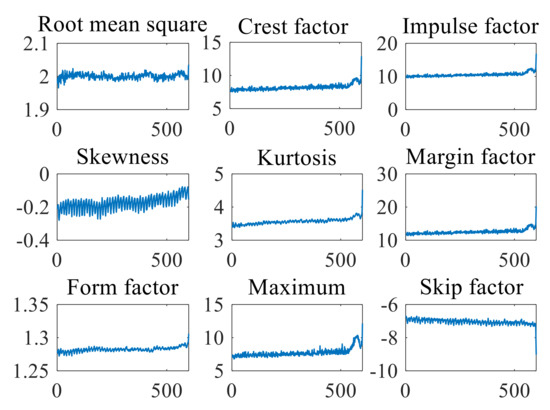
Figure 11. Features of the degradation process data extracted.

In order to reduce the computational burden, these high-dimensional features need to be fused to form a synthetic HI. In this paper, the Mahalanobis distance (MD) method is used to construct the HI [29,30]:

$$M{D}_i=\frac{1}{m}{Z}_i^T{\Sigma }_Z^{-1}{Z}_i,$$

(32)

where $M{D}_i$ is the MD calculated at the $i$-th moment, $Z_i=[z_{i,1},z_{i,2},\dots ,z_{i,m}]$ are the $m$ features extracted at the $i$-th moment in time, and ${\Sigma }_Z$ is the covariance matrix of $Z_i$. The new HI is obtained by calculating the MD of Equation (32), and the result is shown in Figure 12.

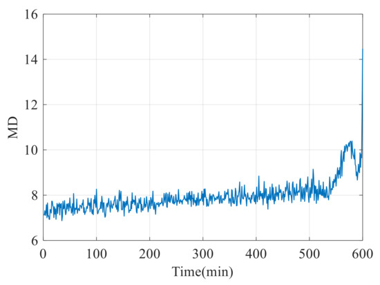
Figure 12. HI constructed by MD.

The extracted features are fused by the MD method as the HI, which is used to describe the degradation process in the RUL prediction.

4.3. RUL Prediction

The MD method is used to perform the fusion of the features extracted from the gearbox vibration signal into an HI, which is often used to predict the RUL. When the failure threshold is set to 10 units of HI value, the corresponding fault occurs at 566 min. For the parameter estimation, we give the concrete expression of the adaptive drift coefficient. The specific estimation results of the unknown parameters $\Phi =[{\mu }_a,{\sigma }_a^2,{\sigma }^2,H,D{]}^T$ of the adaptive GC model are given in Table 4. The GC model, fractional Brownian motion (FBM) model, long short-term memory (LSTM) model and adaptive Wiener are selected for comparison with the adaptive GC model [31,32]. The difference between the GC model and the adaptive GC model is that the adaptive GC model takes into account the time variation of the drift coefficient.

Table 4. Parameters Estimation of Different Prediction Models.

Parameters	${\mathit{\mu }}_{\mathit{a}}$	${\mathit{\sigma }}_{\mathit{a}}$	$\mathit{a}$	$\mathit{\sigma }$	$\mathit{H}$	$\mathit{D}$
adaptive GC model	0.0635	1.2670	-	1.9643	0.5723	1.4523
GC model	−	−	0.0651	2.0617	0.5723	1.4523
FBM model	−	−	0.0592	1.9643	0.5723	−
Adaptive Wiener	0.01163	1.0274	−	1.8640	−	−

From the estimated parameter value if $0<(4-2D)(2-2H)=0.9370\le 1$, the gearbox degradation process has an LRD characteristic. Therefore, the adaptive GC model with an LRD characteristic can be used to predict the gearbox RUL. The estimation of the Hurst exponent $H$ by the RS Method is shown in Figure 13.

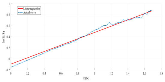
Figure 13. RS method to estimate the Hurst exponent $H$.

According to Equation (24), the estimated value of the Hurst exponent $H$ is the slope in Figure 13. The calculated result is 0.5723. The predicted RUL is obtained through 1000 trials of Monte Carlo simulation [28,33]. The histogram and PDF of 100 RUL prediction are shown in Figure 14.

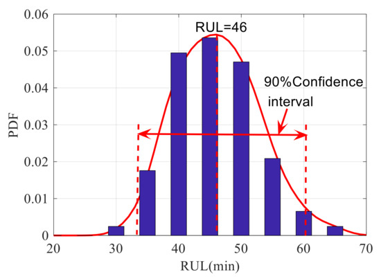
Figure 14. The histogram and PDF of the 100 predicted RUL values.

As shown in Figure 14, according to the statistical results, the RUL has the largest value of the PDF in 46. Hence, the RUL estimate from Monte Carlo simulation is 46. Since the sampling interval is minutes, all RUL values in this work are given in minutes. Then, the PDF of the RUL at 10 different prediction starting points of the operation process is obtained by Monte Carlo simulation. The prediction results of the PDFs by different models are shown in Figure 15 [34,35,36,37].

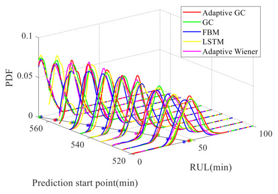
Figure 15. The PDFs of the RUL of different prediction models.

In Figure 15, the black straight line represents the actual RUL, and the five-colored star represents the estimated RUL. The RUL obtained by the five different prediction models is expressed in a two-dimensional plane, and the results are shown in Figure 16. The estimated RUL value of the different models are shown in Table 5.

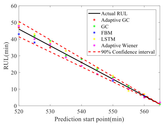
Figure 16. The RUL estimated by different prediction models.

Table 5. The RUL Values Estimated by Different Prediction Models.

Prediction Start Point (min)	Actual RUL (min)	Adaptive GC (min)	GC (min)	FBM (min)	LSTM (min)	Adaptive Wiener (min)
520	46	47	48	43	49	48
525	41	42	42	38	43	40
530	36	35	39	37	38	37
535	31	30	30	33	33	29
540	26	26	28	24	24	24
545	21	22	22	19	23	19
550	16	15	17	15	18	16
555	11	10	12	10	9	10
560	6	5	6	6	7	5
565	1	2	1	2	2	2

To comprehensively compare the prediction advantage of the different models, the evaluation indicators of mean absolute error (MAE), root mean square error (RMSE) and health degree (HD) are considered as follows [38]:

$$MAE=\frac{1}{s}{\displaystyle {\sum }_{i=1}^s\left|L_k-L_k^{*}\right|},$$

(33)

$$RMSE=\sqrt{\frac{1}{s}{\displaystyle {\sum }_{i=1}^s{(L_k-L_k^{*})}^2}},$$

(34)

$$HD=1-\frac{{\displaystyle {\sum }_{i=1}^s{(L_k-L_k^{*})}^2}}{{\displaystyle {\sum }_{i=1}^s{(L_k-{\overline{L}}_k)}^2}},$$

(35)

where $L_k$ is the predicted RUL, $L_k^{*}$ is the actual RUL, $s$ is the number of predictions and ${\overline{L}}_k$ is the mean value of $L_k$.

In Table 6, the RUL prediction accuracy of the adaptive GC model is higher than that of the other four models. One of the reasons is that the drift coefficient of the adaptive GC model has been adaptively updated on the data collected, which gives a more accurate description of the degradation trend of the gearboxes with a fixed drift coefficient. Another reason is that it is more accurate to use an adaptive GC model with LRD characteristics to predict the degradation process of wind turbine gearboxes with LRD characteristics.

Table 6. Prediction Accuracy of the Five Models.

Prediction Models	MAE	RMSE	HD
Adaptive GC	0.9000	0.9487	0.0012
GC	1.2000	1.4832	0.0409
FBM	1.6000	1.8439	0.0373
LSTM	1.9000	1.9748	0.0476
Adaptive Wiener	1.3000	1.4491	0.0112

5. Conclusions, Limitations and Future Research

Based on the GC process, an adaptive GC model with LRD characteristics and randomness is originally proposed for RUL prediction of the gearboxes in a wind turbine. The general conclusions of the work related to such model are as follows:

• The degradation of wind turbine gearboxes is a slow and continuous process with LRD characteristics. The LRD is demonstrated by the Hurst exponent and the fractal dimension. The randomness is explained by the diffusion term driven by the GC difference time sequence. In this paper, the GC difference time sequence is constructed through the ACF of the GC process, and the normality of the time sequence is verified;
• The adaptability of the adaptive GC model is manifested by using time-varying drift coefficients to update the degradation trend in real time so as to improve prediction accuracy. The expressions for the adaptive estimation of the unknown parameters and RUL are derived. The upgradation of the parameters is beneficial to the research of RUL prediction compared with the models of fixed parameters;
• The upgrading of the drift coefficient is based on the random sampling of the Gaussian distribution, which brings little error. Future work can focus on a better upgradation of the drift coefficient.

References

- Wang, J.; Peng, Y.; Wei, Q. Current-Aided Order Tracking of Vibration Signals for Bearing Fault Diagnosis of Direct-Drive Wind Turbines. IEEE Trans. Ind. Electron. 2016, 63, 6336–6346. [Google Scholar] [CrossRef]
- Chen, J.; Pan, J.; Li, Z. Generator bearing fault diagnosis for wind turbine via empirical wavelet transform using measured vibration signals-ScienceDirect. Renew. Energy 2016, 89, 80–92. [Google Scholar] [CrossRef]
- Xu, M.; Baraldi, P.; Al-Dahidi, S. Fault prognostics by an ensemble of Echo State Networks in presence of event-based measurements. Eng. Appl. Artif. Intell. 2020, 87, 103346.1–103346.15. [Google Scholar] [CrossRef]
- Wen, P.; Zhao, S.; Chen, S. A generalized remaining useful life prediction method for complex systems based on composite health indicator. Reliab. Eng. Syst. Saf. 2021, 205, 107241. [Google Scholar] [CrossRef]
- Si, X.S.; Wang, W.; Hu, C.H. Remaining Useful Life Estimation Based on a Nonlinear Diffusion Degradation Process. IEEE Trans. Reliab. 2012, 61, 50–67. [Google Scholar] [CrossRef]
- Gearboxes Reliability Database. Available online: https://grd.nrel.gov/#/stats (accessed on 20 June 2021).
- Luo, L.; Peng, X.; Tong, C. A multigroup framework for fault detection and diagnosis in large-scale multivariate systems. J. Process Control. 2021, 100, 65–79. [Google Scholar] [CrossRef]
- Li, J.; Chen, X.; Du, Z. A new noise-controlled second-order enhanced stochastic resonance method with its application in wind turbine drivetrain fault diagnosis. Renew. Energy 2013, 60, 7–19. [Google Scholar] [CrossRef]
- Cheng, F.; Peng, Y.; Qu, L. Current-Based Fault Detection and Identification for Wind Turbine Drivetrain Gearboxes. IEEE Trans. Ind. Appl. 2017, 53, 878–887. [Google Scholar] [CrossRef]
- Gao, Q.W.; Liu, W.Y.; Tang, B.P. A novel wind turbine fault diagnosis method based on intergral extension load mean decomposition multiscale entropy and least squares support vector machine. Renew. Energy 2018, 116, 169–175. [Google Scholar] [CrossRef]
- Rezamand, M.; Kordestani, M.; Carriveau, R. An Integrated Feature-Based Failure Prognosis Method for Wind Turbine Bearings. IEEE Trans. Mechatron. 2020, 25, 1468–1478. [Google Scholar] [CrossRef]
- Ruiz, G.C.R. Sound and vibration-based pattern recognition for wind turbines driving mechanisms. Renew. Energy 2017, 109, 262–274. [Google Scholar] [CrossRef]
- Wang, J.; Liang, Y.; Zheng, Y. An integrated fault diagnosis and prognosis approach for predictive maintenance of wind turbine bearing with limited samples. Renew. Energy 2020, 145, 642–650. [Google Scholar] [CrossRef]
- Limon, S.; Yadav, O.P. Predicting remaining lifetime using the monotonic gamma process and bayesian inference for multi-stress conditions. Procedia Manuf. 2019, 38, 1260–1267. [Google Scholar] [CrossRef]
- Peng, W.; Zhu, S.P.; Shen, L. The transformed inverse Gaussian process as an age- and state-dependent degradation model. Appl. Math. Model. 2019, 75, 837–852. [Google Scholar] [CrossRef]
- Kong, D.; Balakrishnan, N.; Cui, L. Two-Phase Degradation Process Model with Abrupt Jump at Change Point Governed by Wiener Process. IEEE Trans. Reliab. 2017, 66, 1345–1360. [Google Scholar] [CrossRef]
- Carrillo, R.E.; Aysal, T.C.; Barner, K.E. A generalized Cauchy distribution framework for problems requiring robust behavior. EURASIP J. Adv. Signal Process. 2010, 2010, 312989. [Google Scholar] [CrossRef]
- Liu, H.; Song, W.Q.; Zhang, Y.J. Generalized Cauchy degradation model with long-range dependence and maximum Lyapunov exponent for remaining useful life. IEEE Trans. Instrum. Meas. 2021, 70, 3512812. [Google Scholar] [CrossRef]
- Lim, S.; Li, M. A generalized Cauchy process and its application to relaxation phenomena. J. Phys. A Math. Gen. 2006, 39, 2935–2951. [Google Scholar] [CrossRef]
- Li, M.; Li, J.Y. Generalized Cauchy model of sea level fluctuations with long-range dependence. Phys. A Stat. Mech. Appl. 2017, 484, 309–335. [Google Scholar] [CrossRef]
- Kurita, E.; Seo, T. Multivariate normality test based on kurtosis with two-step monotone missing data. J. Multivar. Anal. 2021, 188, 104824. [Google Scholar] [CrossRef]
- Dimitrova, D.S.; Kaishev, V.K.; Tan, S. Computing the Kolmogorov-Smirnov Distribution When the Underlying CDF is Purely Discrete. Mixed, or Continuous. J. Stat. Softw. 2020, 95, 1–42. [Google Scholar] [CrossRef]
- Zhang, Z.; Si, X.; Hu, C. Degradation Data Analysis and Remaining Useful Life Estimation: A Review on Wiener-Process-Based Methods. Eur. J. Oper. Res. 2018, 271, 775–796. [Google Scholar] [CrossRef]
- Hong, G.X.; Song, W.Q.; Gao, Y. An Iterative Model of the Generalized Cauchy Process for Predicting the Remaining Useful Life of Lithium-ion Batteries. Measurement 2022, 187, 110269. [Google Scholar] [CrossRef]
- Song, W.Q.; Liu, H.; Zio, E. Long-range dependence and heavy tail characteristics for remaining useful life prediction in rolling bearing degradation. Appl. Math. Model. 2022, 102, 268–284. [Google Scholar] [CrossRef]
- Duan, S.W.; Song, W.Q.; Zio, E. Product technical life prediction based on multi-modes and fractional Levy stable motion. Mech. Syst. Signal Process. 2021, 161, 107974. [Google Scholar] [CrossRef]
- Lei, Y.G.; Li, N.P.; Guo, L. Machinery health prognostics: A systematic review from data acquisition to RUL prediction. Mech. Syst. Signal Process. 2018, 104, 799–834. [Google Scholar] [CrossRef]
- Cheng, Y.; Zhu, H.; Hu, K. Reliability prediction of machinery with multiple degradation characteristics using double-Wiener process and Monte Carlo algorithm. Mech. Syst. Signal Process. 2019, 134, 106333. [Google Scholar] [CrossRef]
- Wang, Y.; Peng, Y.Z.; Zi, Y.Y. A Two-Stage Data-Driven-Based Prognostic Approach for Bearing Degradation Problem. IEEE Trans. Ind. Inform. 2016, 12, 924–932. [Google Scholar] [CrossRef]
- Azevedo, H.; Araujo, A.; Bouchonneau, N. A review of wind turbine bearing condition monitoring: State of the art and challenges. Renew. Sustain. Energy Rev. 2016, 56, 368–379. [Google Scholar] [CrossRef]
- Zhang, H.; Chen, M.; Xi, X. Remaining Useful Life Prediction for Degradation Processes with Long-Range Dependence. IEEE Trans. Reliab. 2017, 66, 1368–1379. [Google Scholar] [CrossRef]
- Fu, S.; Zhang, Y.; Lin, L. Deep Residual LSTM with Domain-invariance for Remaining Useful Life Prediction Across Domains. Reliab. Eng. Syst. Saf. 2021, 216, 108012. [Google Scholar] [CrossRef]
- Xing, X.; Feng, Q.; Zhang, W. Vapor-liquid equilibrium and criticality of CO2 and n-heptane in shale organic pores by the Monte Carlo simulation. Fuel 2021, 299, 120909. [Google Scholar] [CrossRef]
- Jie, X.; Song, W.Q.; Francesco, V. Generalized Cauchy Process: Difference Iterative Forecasting Model. Fractal Fract. 2021, 5, 38. [Google Scholar] [CrossRef]
- Li, X.; Ma, Y. Remaining useful life prediction for lithium-ion battery using dynamic fractional brownian motion degradation model with long-term dependence. J. Power Electron. 2022. [Google Scholar] [CrossRef]
- Sayah, M.; Guebli, D.; Masry, Z.A.; Zerhoui, N. Robustness testing framework for RUL prediction Deep LSTM networks. ISA Trans. 2021, 113, 28–38. [Google Scholar] [CrossRef]
- Zhai, Q.Q.; Ye, Z.S. RUL Prediction of Deteriorating Products Using an Adaptive Wiener Process Model. IEEE Trans. Ind. Inform. 2017, 13, 2911–2921. [Google Scholar] [CrossRef]
- Cheng, F.; Qu, L.; Qiao, W. Fault Prognosis and Remaining Useful Life Prediction of Wind Turbine Gearboxes Using Current Signal Analysis. IEEE Trans. Sustain. Energy 2018, 9, 157–167. [Google Scholar] [CrossRef]
Publisher’s Note: MDPI stays neutral with regard to jurisdictional claims in published maps and institutional affiliations. |
© 2022 by the authors. Licensee MDPI, Basel, Switzerland. This article is an open access article distributed under the terms and conditions of the Creative Commons Attribution (CC BY) license (https://creativecommons.org/licenses/by/4.0/).