A Neutrosophic Cubic Hesitant Fuzzy Decision Support System, Application in the Diagnosis and Grading of Prostate Cancer

Abstract

According to available estimates with WHO, cancers are the sixth leading cause of global human morbidity and mortality. Prostate Cancer is the fifth-ranked most lethal among various cancers, and hence it warrants serious, dedicated research for improving its early detection. The employed methodologies such as prostate-specific antigen test, Gleason Score, and T2 Staging lack precision and accuracy in conditions where information is scarring, vague and uncertain. Consequently, in the present study, the innovative use of neutrosophic cubic fuzzy sets (NCFS) is employed to improve prostate cancer detection in situations where basic information is vague, imprecise, and uncertain. Specific and critical similarity measures are defined for using NCFS methodology for the evaluation of prostate cancer. This methodology is found reasonably better compared to the existing benchmark methods for the detection and grading of prostate cancer.

1. Introduction

Prostate cancer is a cancer of prostate glands found only in men and is the fifth largest cause of cancer-based deaths in males globally. The co-occurrence of high-grade depression further aggravates the condition, and hence a significantly increased rate of mortality is reported with prostate cancer [1]. A study reported from the UK found that more than 37,000 new cases of prostate cancer are registered in that country annually (Torre et al. [2]). This situation is further complicated as the age of men increases, i.e., with increased age, the risk of prostate cancer is increased (Jemal et al. [3]). Thus, for better management and effective treatment of prostate cancer, early-stage detection methodologies are very critical (Cartel et al. [4]), and improvements in the existing detection and staging methodologies are also the cry of the hour. In this context, Cao et al. [5] discuss several markers which are useful in the early stage detection of prostate cancer. A variety of methodologies and tests are used for early detection and staging of prostate cancer to determine whether metastasis has taken place or not. The prostate-specific antigen test for detection (Kelly et al. [6]) and Gleason Scoring System (Chan et al. [7]) for determination of Staging/grading prostate cancer are commonly employed approaches. The Gleason Score Range (from 2 to 10) helps stage prostate cancer and works based on tumor-nodes-metastasis (TNM) and is the standardized methodology recommended by the American Joint Committee on Cancer Staging System (Edge et al. [8]). In this staging system, six to twelve T2 staging samples are harvested from the prostate gland to detect cancerous diffusions. The positive results are reflections from samples harvested from both lobes of the prostate gland with specific T2 staging Scores, Gleason Scores, and also the initial PSA test (Partin et al. [9,10,11]). Additional details are described elsewhere [12,13,14,15,16]. The real problem with these methods is when the information becomes scarred, uncertain, non-consistent, and diffuse. Thus, new methodologies and approaches are badly required in uncertain conditions for accuracy of results needed for proper decision-making where a suspected patient may have prostate cancer and warrants early and accurate detection. It is a foregone conclusion that early detection of prostate cancer is vital for proper management of the pathology and reduction of the rate of mortality with this disease. Fuzzy Sets methodology is applied where uncertainty exists. The studies reported by Serita et al. [17,18] make the use of fuzzy sets for the detection of prostate cancer. Similarly, Benecchi [19] reported neuro-fuzzy sets for early detection and staging of prostate cancer, whereas Seker et al. [20] described their method for early detection and staging of prostate cancer which is based upon fuzzy logic. Jing et al. [21] have also reported some improvements in methodology based upon the use of cubic-hesitant-fuzzy sets by measuring the similarities. More details about neutrosophic’s theories can be seen in [22,23,24,25]. Fu et al. established a useful evaluation method of risk grades for prostate cancer using a similarity measure of cubic hesitant fuzzy sets [21]. Thai and Huh discussed optimizing techniques for patient transportation by applying cloud computing [26]. Fu et al. established an evaluation method of benign prostatic hyperplasia using cubic hesitant fuzzy sets [27]. Fu and Ye established a similarity measure with indeterminate parameters of cubic hesitant neutrosophic numbers and its risk grade assessment approach for prostate cancer patients [28]. Choi and Huh established useful techniques to reduce STD infections [29]. Ho and Thanh discussed a community interests approach to a topic model with time factor and clustering methods [30]. Kadian and Kumar established novel intuitionistic Renyi’s–Tsallis discriminant information measure and discussed its applications in decision-making [31]. The contributions of different researchers using different versions of fuzzy sets can be seen in [32,33,34,35,36].

In the present study, we present a new innovative method, and the concept is based upon neutrosophic-cubic-hesitant-fuzzy sets (NCHFS) by making use of the Neutrosophic Theory of Smarandache [22]. The NCHFS combines the advantages of NCS and hesitant fuzzy set. This characteristic makes the NCHFS a powerful tool to deal with inconsistent data. Many multi attribute decision-making methods often ignore the uncertainty and hence yield the results that are not reliable. The NCHFS can efficiently handle the complex information in a decision-making problem. Our results show significant improvement concerning existing prostate cancer detection and staging methodologies in conditions where information is scarce, uncertain, and indeterminate.

2. Preliminaries

In this section, we have collected some helpful material from the existing literature.

Definition 1 ([22]).

A neutrosophic set (NS) in a fixed non empty set U is the structure of the form $\mathcal{N}=\{\langle \left({\mathcal{N}}_T\right)\left(u\right),\left({\mathcal{N}}_I\right)\left(u\right),\left({\mathcal{N}}_F\right)\left(u\right)/u\in U\}$ where ${\mathcal{N}}_T:U⟶[0,1]$ is called truth membership function $,{\mathcal{N}}_I:U⟶[0,1]$ is called indeterminate membership function, ${\mathcal{N}}_F:U⟶[0,1]$ is called false membership function, and ${\mathcal{N}}_T,$${\mathcal{N}}_I$ and ${\mathcal{N}}_F$ are the single fuzzy valued in $[0,1]$.

Definition 2 ([25]).

An interval neutrosophic set (INS) in a fixed non empty set U is the structure of the form $\tilde{\mathcal{N}}=\left\{〈{\tilde{\mathcal{N}}}_T\left(u\right),{\tilde{\mathcal{N}}}_I\left(u\right),{\tilde{\mathcal{N}}}_F\left(u\right)〉/u\in U\right\}$ where ${\tilde{\mathcal{N}}}_T:U⟶D[0,1],{\tilde{\mathcal{N}}}_I:U⟶D[0,1]$ and ${\tilde{\mathcal{N}}}_F:U⟶D[0,1]$ are respectively called interval-truth membership function, an interval-indeterminacy membership function and interval-falsity membership function, and it is denoted by ${\tilde{\mathcal{N}}}_T=[{\mathcal{N}}^{-},{\mathcal{N}}^{+}]\subseteq [0,1],$${\tilde{\mathcal{N}}}_I=[{\mathcal{N}}^{-},{\mathcal{N}}^{+}]\subseteq [0,1]$ and ${\tilde{\mathcal{N}}}_F=[{\mathcal{N}}^{-},{\mathcal{N}}^{+}]\subseteq [0,1].$

Definition 3 ([32]).

A hesitant fuzzy set (HFS) in a fixed non empty set U, is of the form $\mathcal{H}=\left\{(h,f(u\left)\right)/u\in U and f\left(h\right)\in [0,1]\right\}$ where $f\left(h\right)$ is a finite set of values in $[0,1].$

Definition 4 ([33]).

A cubic set (CS) in a fixed non empty set U is the structure of the following form: $\mathcal{C}=\{〈\tilde{\mathcal{A}}\left(u\right),\mathcal{A}\left(u\right)〉/u\in U\}$ where $\tilde{\mathcal{A}}:U⟶D[0,1]$ is an interval-valued fuzzy set in U and $\mathcal{A}:U⟶[0,1]$ is a fuzzy set in U.

Definition 5 ([21]).

A cubic hesitant fuzzy set (CHFS) in a fixed non empty set U is the structure of the form $\mathcal{CH}=\left\{〈\tilde{r}\left(u\right),r_1\left(u\right),r_2\left(u\right),r_3\left(u\right),\dots ,r_n\left(u\right)〉/u\in U\right\}$ where $\tilde{r}:U⟶D[0,1]$ is an interval-valued fuzzy set and $r_i:U⟶[0,1]$ for $i=1,2,\dots ,n$ is a finite set of some different values in $[0,1]$.

Definition 6 ([23]).

Let U be a non-empty set. A neutrosophic hesitant fuzzy set (NHFS) in a fixed non empty set U is the structure of the form

$$\mathcal{NCH}=\left\{〈\begin{array}{c}{\left\{{\mathcal{NH}}_1\left(u\right),{\mathcal{NH}}_2\left(u\right),{\mathcal{NH}}_3\left(u\right),\dots ,{\mathcal{NH}}_n\left(u\right)\right\}}_T,\\ {\left\{{\mathcal{NH}}_1\left(u\right),{\mathcal{NH}}_2\left(u\right),{\mathcal{NH}}_3\left(u\right),\dots ,{\mathcal{NH}}_n\left(u\right)\right\}}_I,\\ {\left\{{\mathcal{NH}}_1\left(u\right),{\mathcal{NH}}_2\left(u\right),{\mathcal{NH}}_3\left(u\right),\dots ,{\mathcal{NH}}_n\left(u\right)\right\}}_F\end{array}〉;u\in U\right\}$$

where ${\mathcal{NH}}_i{\left(u\right)}_T,{\mathcal{NH}}_i{\left(u\right)}_I,{\mathcal{NH}}_i{\left(u\right)}_F\in [0,1]$ for $i=1,2,3,\dots ,n$ are the finite set of values in $[0,1]$, called the truth hesitant membership function, indeterminacy hesitant membership function and falsity hesitant membership functions.

3. Neutrosophic Cubic Hesitant Fuzzy Sets (NCHFSs)

Before discussing the evaluation method for the risk grade of PC’s patient, in this section, we provide the concept of the neutrosophic cubic hesitant fuzzy set, which is an extension of the cubic hesitant fuzzy set. We also define external and internal neutrosophic cubic hesitant fuzzy sets and discuss some basic properties.

Definition 7.

Let U be a non-empty set. A neutrosophic cubic hesitant fuzzy set (NCHFS) is a pair $\mathcal{NCH}=(\tilde{\mathcal{M}},\mathcal{M})$ where $\tilde{\mathcal{M}}=\{〈{\tilde{\mathcal{M}}}_T\left(u\right),{\tilde{\mathcal{M}}}_I\left(u\right),{\tilde{\mathcal{M}}}_F\left(u\right)〉/u\in U\}$ as an interval neutrosopohic set (INS) in U and

$$\mathcal{M}=\{〈\begin{array}{c}{\left\{{\mathcal{M}}_1\left(u\right),{\mathcal{M}}_2\left(u\right),{\mathcal{M}}_3\left(u\right),\dots ,{\mathcal{M}}_n\left(u\right)\right\}}_T,\\ {\left\{{\mathcal{M}}_1\left(u\right),{\mathcal{M}}_2\left(u\right),{\mathcal{M}}_3\left(u\right),\dots ,{\mathcal{M}}_n\left(u\right)\right\}}_I,\\ {\left\{{\mathcal{M}}_1\left(u\right),{\mathcal{M}}_2\left(u\right),{\mathcal{M}}_3\left(u\right),\dots ,{\mathcal{M}}_n\left(u\right)\right\}}_F\end{array}〉/u\in U\}$$

as a neutrosopohic hesitant fuzzy set (NHFS) in U. Then, each element of $\mathcal{NCH}=(\tilde{\mathcal{M}},\mathcal{M})$ is simply denoted by $\tilde{\mathcal{M}}=〈[m_1^{*},m_2^{**}],[m_3^{*},m_4^{**}],[m_5^{*},m_6^{**}]〉$ and $\mathcal{M}=〈(n_1^{*},n_2^{*},\dots ,n_p^{*}),(n_1^{**},n_2^{**},\dots n_p^{**}),(n_1^{***},n_2^{***},\dots ,n_p^{***})〉$ or

$$\mathcal{NCH}=\left\{\begin{array}{c}[m_1^{*},m_2^{**}],[m_3^{*},m_4^{**}],[m_5^{*},m_6^{**}],\\ (n_1^{*},n_2^{*},\dots ,n_p^{*}),(n_1^{**},n_2^{**},\dots n_p^{**}),(n_1^{***},n_2^{***},\dots ,n_p^{***}),\end{array}\right\}$$

which is called neutrosophic cubic hesitant fuzzy number (NCHFN).

Definition 8.

A neutrosophic cubic hesitant fuzzy number (NCHFNs) $\mathcal{NCH}=(\tilde{\mathcal{M}},\mathcal{M})$ is called

• Truth-internal neutrosophic cubic hesitant fuzzy number (T-internal) if the following inequality is satisfied $(\forall u\in U)(m_1^{*}\left(u\right)\le (n_1^{*},n_2^{*},\dots ,n_p^{*})\left(u\right)\le m_2^{**}\left(u\right)))$;
• Indeterminacy-internal neutrosophic cubic hesitant fuzzy number (I-internal) if the following inequality is satisfied $(\forall u\in U)(m_3^{*}\left(u\right)\le (n_1^{**},n_2^{**},\dots n_p^{**})\left(u\right)\le m_4^{**}\left(u\right)));$
• Falsity-internal neutrosophic cubic hesitant fuzzy number (F-internal) if the following inequality is satisfied $(\forall u\in U)(m_5^{*}\left(u\right)\le (n_1^{***},n_2^{***},\dots ,n_p^{***})\left(u\right)\le m_6^{**}\left(u\right));$
• A neutrosophic cubic hesitant fuzzy number (NCHFNs) is called internal neutrosophic cubic hesitant fuzzy number if it is T-internal, I-internal, and F-internal.

Definition 9.

A neutrosophic cubic hesitant fuzzy number (NCHFNs) $\mathcal{NCH}=(\tilde{\mathcal{M}},\mathcal{M})$ is called,

• Truth-external neutrosophic cubic hesitant fuzzy number (T-external) if the following inequality is satisfied $(\forall u\in U)(n_1^{*},n_2^{*},\dots ,n_p^{*})\left(u\right)\notin (m_1^{*},m_2^{**})\left(u\right);$
• Indeterminacy-external neutrosophic cubic hesitant fuzzy number (I-external) if the following inequality is satisfied $(\forall u\in U)(n_1^{**},n_2^{**},\dots n_p^{**})\left(u\right)\notin (m_3^{*},m_4^{**})\left(u\right);$
• Falsity-external neutrosophic cubic hesitant fuzzy number (F-external) if the following inequality is satisfied $(\forall u\in U)(n_1^{***},n_2^{***},\dots ,n_p^{***})\left(u\right)\notin (m_5^{*},m_6^{**})\left(u\right);$
• A neutrosophic cubic hesitant fuzzy number (NCHFN) is called external neutrosophic cubic hesitant fuzzy number if it is T-external, I-external, and F-external.

Definition 10.

Let ${\mathcal{NCH}}_1=({\tilde{\mathcal{M}}}_1,{\mathcal{M}}_1)=\left\{\begin{array}{c}[m_1^{*},m_2^{**}],[m_3^{*},m_4^{**}],[m_5^{*},m_6^{**}],(n_1^{*},n_2^{*},\dots ,n_p^{*}),\\ (n_1^{**},n_2^{**},\dots n_p^{**}),(n_1^{***},n_2^{***},\dots ,n_p^{***})\end{array}\right\}$ and ${\mathcal{NCH}}_2=({\tilde{\mathcal{M}}}_2,{\mathcal{M}}_2)=\left\{\begin{array}{c}[r_1^{*},r_2^{**}],[r_3^{*},r_4^{**}],[r_5^{*},r_6^{**}],(s_1^{*},s_2^{*},\dots ,s_p^{*}),\\ (s_1^{**},s_2^{**},\dots s_p^{**}),(s_1^{***},s_2^{***},\dots ,s_p^{***})\end{array}\right\}$ be two neutrosophic cubic hesitant fuzzy numbers (NCHFNs). Then, we define

(1) if ${\mathcal{NCH}}_1={\mathcal{NCH}}_2$ then $({\tilde{\mathcal{M}}}_1,{\mathcal{M}}_1)=({\tilde{\mathcal{M}}}_2,{\mathcal{M}}_2)$ i.e, $[m_1^{*},m_2^{**}]=[r_1^{*},r_2^{**}],[m_3^{*},m_4^{**}]=[r_3^{*},r_4^{**}]$ and $[m_5^{*},m_6^{**}]=[r_5^{*},r_6^{**}]$ similarly $\left(n_k^{*}\right)=\left(s_k^{*}\right),$$\left(n_k^{**}\right)=\left(s_k^{**}\right)$ and $\left(n_k^{***}\right)=\left(s_k^{***}\right)(\forall$$k=1,2,3,\dots ,p).$

(2) if ${\mathcal{NCH}}_1\subseteq {\mathcal{NCH}}_2$, then $({\tilde{\mathcal{M}}}_1,{\mathcal{M}}_1)\subseteq ({\tilde{\mathcal{M}}}_2,{\mathcal{M}}_2)$ i.e., $[m_1^{*},m_2^{**}]\subseteq [r_1^{*},r_2^{**}],[m_3^{*},m_4^{**}]\subseteq [r_3^{*},r_4^{**}]$ and $[m_5^{*},m_6^{**}]\subseteq [r_5^{*},r_6^{**}]$ while $\left(n_k^{*}\right)\le \left(s_k^{*}\right),$$\left(n_k^{**}\right)\le \left(s_k^{**}\right)$ and $\left(n_k^{***}\right)\le \left(s_k^{***}\right)(\forall$$k=1,2,3,\dots ,p).$

(3) ${\mathcal{NCH}}_1^C=〈{\tilde{\mathcal{M}}}_1^C,{\mathcal{M}}_1^C〉=[1-m_2^{**},1-m_1^{*}],[1-m_4^{**},1-m_3^{*}],[1-m_6^{**},1-m_5^{*}],(1-n_p^{*},1-n_{p-1}^{*},\dots ,1-n_1^{*})$, $(1-n_p^{**},1-n_{p-1}^{**},\dots ,1-n_1^{**})$ and $(1-n_p^{***},1-n_{p-1}^{***},\dots ,1-n_1^{***})$ (complement of ${\mathcal{NCH}}_1$).

4. Similarity Measures of NCHFSs

Here, we discussed some similarity measures of neutrosophic cubic hesitant fuzzy sets (NCHFSs) that will be used in the next section:

Definition 11.

Let ${\mathcal{NCH}}_1=({\tilde{\mathcal{M}}}_1,{\mathcal{M}}_1)=\left\{\begin{array}{c}[m_1^{*},m_2^{**}],[m_3^{*},m_4^{**}],[m_5^{*},m_6^{**}],(n_1^{*},n_2^{*},\dots ,n_p^{*}),\\ (n_1^{**},n_2^{**},\dots n_p^{**}),(n_1^{***},n_2^{***},\dots ,n_p^{***})\end{array}\right\}$ and ${\mathcal{NCH}}_2=({\tilde{\mathcal{M}}}_2,{\mathcal{M}}_2)=\left\{\begin{array}{c}[r_1^{*},r_2^{**}],[r_3^{*},r_4^{**}],[r_5^{*},r_6^{**}],(s_1^{*},s_2^{*},\dots ,s_p^{*}),\\ (s_1^{**},s_2^{**},\dots s_p^{**}),(s_1^{***},s_2^{***},\dots ,s_p^{***})\end{array}\right\}$ be two NCHFNs, and the LCMN of p and q in ${\mathcal{M}}_1$ and ${\mathcal{M}}_2$ is S, then we can extend both by the following forms:

$${\mathcal{NCH}}_1^L=\left\{\begin{array}{c}[m_1^{*},m_2^{**}],[m_3^{*},m_4^{**}],[m_5^{*},m_6^{**}],\\ \stackrel{S}{\overbrace{\left(\begin{array}{c}(n_{11}^{1*},n_{12}^{2*},\dots ,n_{11}^{s/p*}),(n_{12}^{1*},n_{12}^{2*},\dots ,n_{12}^{s/p*}),\dots ,(n_{1p}^{1*},n_{1p}^{2*},\dots ,n_{1p}^{s/p*}),\\ (n_{11}^{1**},n_{12}^{2**},\dots ,n_{11}^{s/p**}),(n_{12}^{1**},n_{12}^{2**},\dots ,n_{12}^{s/p**}),\dots ,(n_{1p}^{1**},n_{1p}^{2**},\dots ,n_{1p}^{s/p**}),\\ (n_{11}^{1***},n_{12}^{2***},\dots ,n_{11}^{s/p***}),(n_{12}^{1***},n_{12}^{2***},\dots ,n_{12}^{s/p***}),\dots ,(n_{1p}^{1***},n_{1p}^{2***},\dots ,n_{1p}^{s/p***}),\end{array}\right)}}\end{array}\right\}$$

and

$${\mathcal{NCH}}_2^L=\left\{\begin{array}{c}[r_1^{*},r_2^{**}],[r_3^{*},r_4^{**}],[r_5^{*},r_6^{**}],\\ \stackrel{S}{\overbrace{\left(\begin{array}{c}(s_{11}^{1*},s_{12}^{2*},\dots ,s_{11}^{s/q*}),(s_{12}^{1*},s_{12}^{2*},\dots ,s_{12}^{s/q*}),\dots ,(s_{1q}^{1*},s_{1q}^{2*},\dots ,s_{1q}^{s/q*}),\\ (s_{11}^{1**},s_{12}^{2**},\dots ,s_{11}^{s/q**}),(s_{12}^{1**},s_{12}^{2**},\dots ,s_{12}^{s/q**}),\dots ,(s_{1q}^{1**},s_{1q}^{2**},\dots ,s_{1q}^{s/q**}),\\ (s_{11}^{1***},s_{12}^{2***},\dots ,s_{11}^{s/q***}),(s_{12}^{1***},s_{12}^{2***},\dots ,s_{12}^{s/q***}),\dots ,(s_{1q}^{1***},s_{1q}^{2***},\dots ,s_{1q}^{s/q***}),\end{array}\right)}}\end{array}\right\}$$

Definition 12.

Let ${\mathcal{NCH}}_1=({\tilde{\mathcal{M}}}_1,{\mathcal{M}}_1)=\left\{\begin{array}{c}[m_1^{*},m_2^{**}],[m_3^{*},m_4^{**}],[m_5^{*},m_6^{**}],(n_1^{*},n_2^{*},\dots ,n_p^{*}),\\ (n_1^{**},n_2^{**},\dots n_p^{**}),(n_1^{***},n_2^{***},\dots ,n_p^{***})\end{array}\right\}$ and ${\mathcal{NCH}}_2=({\tilde{\mathcal{M}}}_2,{\mathcal{M}}_2)=\left\{\begin{array}{c}[r_1^{*},r_2^{**}],[r_3^{*},r_4^{**}],[r_5^{*},r_6^{**}],(s_1^{*},s_2^{*},\dots ,s_p^{*}),\\ (s_1^{**},s_2^{**},\dots s_p^{**}),(s_1^{***},s_2^{***},\dots ,s_p^{***})\end{array}\right\}$ be two NCHFNs, where

$$\begin{array}{ccc}\hfill {\left({\widetilde{{\mathcal{M}}_1}}_k\right)}_T& =& \hfill {[m_k^{*},m_k^{**}]}_T,{\left({\widetilde{{\mathcal{M}}_1}}_k\right)}_I={[m_k^{*},m_k^{**}]}_I and {\left({\widetilde{{\mathcal{M}}_1}}_k\right)}_F={[m_k^{*},m_k^{**}]}_F\hfill \\ \hfill \mathit{where} {\left({\mathcal{M}}_{1k}\right)}_T& =& \hfill {(n_k^1,n_k^2,n_k^3,n_k^4,...,n_k^{p_{1k}})}_T,{\left({\mathcal{M}}_{1k}\right)}_I={(n_k^1,n_k^2,n_k^3,n_k^4,...,n_k^{p_{1k}})}_I, \hfill \\ \hfill {\left({\mathcal{M}}_{1k}\right)}_F& =& \hfill {(n_k^1,n_k^2,n_k^3,n_k^4,...,n_k^{p_{1k}})}_F\hfill \\ \hfill and {\left({\widetilde{{\mathcal{M}}_2}}_k\right)}_T& =& \hfill {[r_k^{*},r_k^{**}]}_T,{\left({\tilde{r}}_k\right)}_I={[r_k^{*},r_k^{**}]}_I and {\left({\tilde{r}}_k\right)}_F={[r_k^{*},r_k^{**}]}_F\hfill \\ \hfill \mathit{where} {\left(r_k\right)}_T& =& \hfill {(s_k^1,s_k^2,s_k^3,s_k^4,...,s_k^{p_{2k}})}_T,{\left(r_k\right)}_I={(s_k^1,s_k^2,s_k^3,s_k^4,...,s_k^{p_{2k}})}_I \hfill \\ \hfill and {\left(r_k\right)}_F& =& \hfill {(s_k^1,s_k^2,s_k^3,s_k^4,...,s_k^{p_{2k}})}_F\hfill \end{array}$$

as $k=1,2,3,\dots ..,m$ and $\alpha >0$; then, the generalized neutrosophic cubic hesitant fuzzy number normalized distance between ${\mathcal{NCH}}_1$ and ${\mathcal{NCH}}_2$ is defined as

$$\begin{array}{ccc}\hfill & & \hfill \mathcal{NCH}{d}_{\alpha }({\mathcal{NCH}}_1,{\mathcal{NCH}}_2)\hfill \end{array}$$

(1)

$$\begin{array}{ccc}& =& \hfill {\left\{{\displaystyle \frac{1}{m}}\sum _{k=1}^m{\displaystyle \frac{1}{(S_k+2)}}\left(\begin{array}{c}{\left|m_k^{*}-r_k^{*}\right|}_T^{\alpha }+{\left|m_k^{**}-r_k^{**}\right|}_T^{\alpha }+{\left|m_k^{*}-r_k^{*}\right|}_I^{\alpha }+{\left|m_k^{**}-r_k^{**}\right|}_I^{\alpha }+\\ {\left|m_k^{*}-r_k^{*}\right|}_F^{\alpha }+{\left|m_k^{**}-r_k^{**}\right|}_F^{\alpha }+\\ {\left|n_k^1-s_k^1\right|}_T^a+{\left|n_k^2-s_k^2\right|}_T^a+{\left|n_k^3-s_k^3\right|}_T^a+,\dots ,{\left|n_k^{S_k}-s_k^{S_k}\right|}_T^a+\\ {\left|n_k^1-s_k^1\right|}_I^a+{\left|n_k^2-s_k^2\right|}_I^a+{\left|n_k^3-s_k^3\right|}_I^a+,\dots ,{\left|n_k^{S_k}-s_k^{S_k}\right|}_I^a+\\ {\left|n_k^1-s_k^1\right|}_F^a+{\left|n_k^2-s_k^2\right|}_F^a+{\left|n_k^3-s_k^3\right|}_F^a+,\dots ,{\left|n_k^{S_k}-s_k^{S_k}\right|}_F^a\end{array}\right)\right\}}^{\frac{1}{\alpha }}\hfill \end{array}$$

(2)

where $S_k$ is the LCMN of $p_{1k}$ and $p_{2k}$ for $k=1,2,3,\dots ,m$ when $\alpha =1,2$ then Equation (1) is reduced to the NCHFN normalized Hamming distance and Euclidean distance as follows: if $\alpha =1$, then Equation (1)

$$\begin{array}{ccc}\hfill & & \hfill d_H({\mathcal{NCH}}_1,{\mathcal{NCH}}_2)\hfill \end{array}$$

(3)

$$\begin{array}{ccc}& =& \hfill \left\{{\displaystyle \frac{1}{m}}\sum _{k=1}^m{\displaystyle \frac{1}{(S_k+2)}}\left(\begin{array}{c}{\left|m_k^{*}-r_k^{*}\right|}_T+{\left|m_k^{**}-r_k^{**}\right|}_T+{\left|m_k^{*}-r_k^{*}\right|}_I+{\left|m_k^{**}-r_k^{**}\right|}_I+\\ {\left|m_k^{*}-r_k^{*}\right|}_F+{\left|m_k^{**}-r_k^{**}\right|}_F+\\ {\left|n_k^1-s_k^1\right|}_T+{\left|n_k^2-s_k^2\right|}_T+{\left|n_k^3-s_k^3\right|}_T+,\dots ,{\left|n_k^{S_k}-s_k^{S_k}\right|}_T+\\ {\left|n_k^1-s_k^1\right|}_I+{\left|n_k^2-s_k^2\right|}_I+{\left|n_k^3-s_k^3\right|}_I+,\dots ,{\left|n_k^{S_k}-s_k^{S_k}\right|}_I+\\ {\left|n_k^1-s_k^1\right|}_F+{\left|n_k^2-s_k^2\right|}_F+{\left|n_k^3-s_k^3\right|}_F+,\dots ,{\left|n_k^{S_k}-s_k^{S_k}\right|}_F\end{array}\right)\right\}\hfill \end{array}$$

(4)

if $\alpha =2$, then Equation (3)

$$\begin{array}{ccc}\hfill & & \hfill d_E({\mathcal{NCH}}_1,{\mathcal{NCH}}_2)\hfill \end{array}$$

(5)

$$\begin{array}{ccc}& =& \hfill {\left\{{\displaystyle \frac{1}{m}}\sum _{k=1}^m{\displaystyle \frac{1}{(S_k+2)}}\left(\begin{array}{c}{\left|m_k^{*}-r_k^{*}\right|}_T^2+{\left|m_k^{**}-r_k^{**}\right|}_T^2+{\left|m_k^{*}-r_k^{*}\right|}_I^2+{\left|m_k^{**}-r_k^{**}\right|}_I^2+\\ {\left|m_k^{*}-r_k^{*}\right|}_F^2+{\left|m_k^{**}-r_k^{**}\right|}_F^2+\\ {\left|n_k^1-s_k^1\right|}_T^2+{\left|n_k^2-s_k^2\right|}_T^2+{\left|n_k^3-s_k^3\right|}_T^2+,\dots ,{\left|n_k^{S_k}-s_k^{S_k}\right|}_T^2+\\ {\left|n_k^1-s_k^1\right|}_I^2+{\left|n_k^2-s_k^2\right|}_I^2+{\left|n_k^3-s_k^3\right|}_I^2+,\dots ,{\left|n_k^{S_k}-s_k^{S_k}\right|}_I^2+\\ {\left|n_k^1-s_k^1\right|}_F^2+{\left|n_k^2-s_k^2\right|}_F^2+{\left|n_k^3-s_k^3\right|}_F^2+,\dots ,{\left|n_k^{S_k}-s_k^{S_k}\right|}_F^2\end{array}\right)\right\}}^{\frac{1}{2}}\hfill \end{array}$$

(6)

The following proposition is related to distance measure $\mathcal{NCH}{d}_{\alpha }({\mathcal{NCH}}_1,{\mathcal{NCH}}_2)$.

Proposition 1.

The following properties on generalized NCHFN normalized distance $\mathcal{NCH}{d}_{\alpha }({\mathcal{NCH}}_1,{\mathcal{NCH}}_2)$ for $\alpha >0$,

(1) $0\le \mathcal{NCH}{d}_{\alpha }({\mathcal{NCH}}_1,{\mathcal{NCH}}_2)\le 1.$

(2) $\mathcal{NCH}{d}_{\alpha }({\mathcal{NCH}}_1,{\mathcal{NCH}}_2)=0$ iff ${\mathcal{NCH}}_1={\mathcal{NCH}}_2.$

(3) $\mathcal{NCH}{d}_{\alpha }({\mathcal{NCH}}_1,{\mathcal{NCH}}_2)=\mathcal{NCH}{d}_{\alpha }({\mathcal{NCH}}_2,{\mathcal{NCH}}_1).$

(4) Let ${\mathcal{NCH}}_1,{\mathcal{NCH}}_2$ and ${\mathcal{NCH}}_3$ be the NCHFS such that ${\mathcal{NCH}}_1\subseteq {\mathcal{NCH}}_2\subseteq {\mathcal{NCH}}_3;$ then, $\mathcal{NCH}{d}_{\alpha }({\mathcal{NCH}}_1,{\mathcal{NCH}}_2)\le \mathcal{NCH}{d}_{\alpha }({\mathcal{NCH}}_1,{\mathcal{NCH}}_3)$ and $\mathcal{NCH}{d}_{\alpha }({\mathcal{NCH}}_2,{\mathcal{NCH}}_3)\le \mathcal{NCH}{d}_{\alpha }({\mathcal{NCH}}_1,{\mathcal{NCH}}_3).$

Proof. 

Clearly $\mathcal{NCH}{d}_{\alpha }({\mathcal{NCH}}_1,{\mathcal{NCH}}_2)$ hold in property (1) to (3) thus, we only proved the property (4). Let ${\mathcal{NCH}}_1,{\mathcal{NCH}}_2$ and ${\mathcal{NCH}}_3$ be the NCHFS such that ${\mathcal{NCH}}_1\subseteq {\mathcal{NCH}}_2\subseteq {\mathcal{NCH}}_3$ we have to show that $\mathcal{NCH}{d}_{\alpha }({\mathcal{NCH}}_1,{\mathcal{NCH}}_2)\le \mathcal{NCH}{d}_{\alpha }({\mathcal{NCH}}_1,{\mathcal{NCH}}_3)$ and $\mathcal{NCH}{d}_{\alpha }({\mathcal{NCH}}_2,{\mathcal{NCH}}_3)\le \mathcal{NCH}{d}_{\alpha }({\mathcal{NCH}}_1,{\mathcal{NCH}}_3).$ Since ${\mathcal{NCH}}_1\subseteq {\mathcal{NCH}}_2\subseteq {\mathcal{NCH}}_3$, then it contains ${\left(m_k^{*}\right)}_T\le {\left(r_k^{*}\right)}_T\le {\left(s_k^{*}\right)}_T,{\left(m_k^{*}\right)}_I\le {\left(r_k^{*}\right)}_I\le {\left(s_k^{*}\right)}_F$ and ${\left(m_k^{*}\right)}_F\le {\left(r_k^{*}\right)}_F\le {\left(s_k^{*}\right)}_F$${\left(m_k^{**}\right)}_T\le {\left(r_k^{**}\right)}_T\le {\left(s_k^{**}\right)}_T,{\left(m_k^{**}\right)}_I\le {\left(r_k^{**}\right)}_I\le {\left(s_k^{**}\right)}_F$ and ${\left(m_k^{**}\right)}_F\le {\left(r_k^{**}\right)}_F\le {\left(s_k^{**}\right)}_F$ and ${\left(n_k^i\right)}_T\le {\left(s_k^i\right)}_T\le {\left({\gamma }_k^i\right)}_T,{\left(n_k^i\right)}_I\le {\left(s_k^i\right)}_I\le {\left({\gamma }_k^i\right)}_I$ and ${\left(n_k^i\right)}_F\le {\left(s_k^i\right)}_F\le {\left({\gamma }_k^i\right)}_F$ for $i=1,2,3,\dots ,s_k$ and $k=1,2,3,\dots ,m.$ Hence, follow the above relations:

$$\begin{array}{ccc}\hfill {\left|m_k^{*}-r_k^{*}\right|}_T^{\alpha }& \le & \hfill {\left|m_k^{*}-s_k^{*}\right|}_T^{\alpha }, {\left|m_k^{**}-r_k^{**}\right|}_T^{\alpha }\le {\left|m_k^{**}-s_k^{**}\right|}_T^{\alpha },\hfill \\ \hfill {\left|m_k^{*}-r_k^{*}\right|}_I^{\alpha }& \le & \hfill {\left|m_k^{*}-s_k^{*}\right|}_I^{\alpha }, {\left|m_k^{**}-r_k^{**}\right|}_I^{\alpha }\le {\left|m_k^{**}-s_k^{**}\right|}_I^{\alpha },\hfill \\ \hfill {\left|m_k^{*}-r_k^{*}\right|}_F^{\alpha }& \le & \hfill {\left|m_k^{*}-s_k^{*}\right|}_F^{\alpha } , {\left|m_k^{**}-r_k^{**}\right|}_F^{\alpha }\le {\left|m_k^{**}-s_k^{**}\right|}_F^{\alpha }\hfill \\ & & \\ \hfill {\left|r_k^{*}-s_k^{*}\right|}_T^{\alpha }& \le & \hfill {\left|m_k^{*}-s_k^{*}\right|}_T^{\alpha } , {\left|r_k^{**}-s_k^{**}\right|}_T^{\alpha }\le {\left|m_k^{**}-s_k^{**}\right|}_T^{\alpha },\hfill \\ \hfill {\left|r_k^{*}-s_k^{*}\right|}_I^{\alpha }& \le & \hfill {\left|m_k^{*}-s_k^{*}\right|}_I^{\alpha } , {\left|r_k^{**}-s_k^{**}\right|}_I^{\alpha }\le {\left|m_k^{**}-s_k^{**}\right|}_I^{\alpha },\hfill \\ \hfill {\left|r_k^{*}-s_k^{*}\right|}_F^{\alpha }& \le & \hfill {\left|m_k^{*}-s_k^{*}\right|}_F^{\alpha } , {\left|r_k^{**}-s_k^{**}\right|}_F^{\alpha }\le {\left|m_k^{**}-s_k^{**}\right|}_F^{\alpha }\hfill \\ & & \\ \hfill {\left|n_k^i-s_k^i\right|}_T^a& \le & \hfill {\left|n_k^i-{\gamma }_k^i\right|}_T^a , {\left|s_k^i-{\gamma }_k^i\right|}_T^a\le {\left|n_k^i-{\gamma }_k^i\right|}_T^a,\hfill \\ \hfill {\left|n_k^i-s_k^i\right|}_I^a& \le & \hfill {\left|n_k^i-{\gamma }_k^i\right|}_I^a , {\left|s_k^i-{\gamma }_k^i\right|}_I^a\le {\left|n_k^i-{\gamma }_k^i\right|}_I^a,\hfill \\ \hfill {\left|n_k^i-s_k^i\right|}_F^a& \le & \hfill {\left|n_k^i-{\gamma }_k^i\right|}_F^a , {\left|s_k^i-{\gamma }_k^i\right|}_F^a\le {\left|n_k^i-{\gamma }_k^i\right|}_F^a\hfill \end{array}$$

Thus, the following inequalities exist:

$$\begin{array}{ccc}\hfill {\left|m_k^{*}-r_k^{*}\right|}_T^{\alpha }+{\left|m_k^{**}-r_k^{**}\right|}_T^{\alpha }+{\left|n_k^i-s_k^i\right|}_T^a& \le & \hfill {\left|m_k^{*}-s_k^{*}\right|}_T^{\alpha }+{\left|m_k^{**}-s_k^{**}\right|}_T^{\alpha }+{\left|n_k^i-{\gamma }_k^i\right|}_T^a,\hfill \\ \hfill {\left|r_k^{*}-s_k^{*}\right|}_T^{\alpha }+{\left|r_k^{**}-s_k^{**}\right|}_T^{\alpha }+{\left|n_k^i-{\gamma }_k^i\right|}_T^a& \le & \hfill {\left|m_k^{*}-s_k^{*}\right|}_T^{\alpha }+{\left|m_k^{**}-s_k^{**}\right|}_T^{\alpha }+{\left|n_k^i-{\gamma }_k^i\right|}_T^a,\hfill \\ & & \\ \hfill {\left|m_k^{*}-r_k^{*}\right|}_I^{\alpha }+{\left|m_k^{**}-r_k^{**}\right|}_I^{\alpha }+{\left|n_k^i-s_k^i\right|}_I^a& \le & \hfill {\left|m_k^{*}-s_k^{*}\right|}_I^{\alpha }+{\left|m_k^{**}-s_k^{**}\right|}_I^{\alpha }+{\left|n_k^i-{\gamma }_k^i\right|}_I^a,\hfill \\ \hfill {\left|r_k^{*}-s_k^{*}\right|}_I^{\alpha }+{\left|r_k^{**}-s_k^{**}\right|}_I^{\alpha }+{\left|n_k^i-{\gamma }_k^i\right|}_I^a& \le & \hfill {\left|m_k^{*}-s_k^{*}\right|}_I^{\alpha }+{\left|m_k^{**}-s_k^{**}\right|}_I^{\alpha }+{\left|n_k^i-{\gamma }_k^i\right|}_I^a,\hfill \\ & & \\ \hfill {\left|m_k^{*}-r_k^{*}\right|}_F^{\alpha }+{\left|m_k^{**}-r_k^{**}\right|}_F^{\alpha }+{\left|n_k^i-s_k^i\right|}_F^a& \le & \hfill {\left|m_k^{*}-s_k^{*}\right|}_F^{\alpha }+{\left|m_k^{**}-s_k^{**}\right|}_F^{\alpha }+{\left|n_k^i-{\gamma }_k^i\right|}_F^a,\hfill \\ \hfill {\left|r_k^{*}-s_k^{*}\right|}_F^{\alpha }+{\left|r_k^{**}-s_k^{**}\right|}_F^{\alpha }+{\left|n_k^i-{\gamma }_k^i\right|}_F^a& \le & \hfill {\left|m_k^{*}-s_k^{*}\right|}_F^{\alpha }+{\left|m_k^{**}-s_k^{**}\right|}_F^{\alpha }+{\left|n_k^i-{\gamma }_k^i\right|}_F^a.\hfill \end{array}$$

for $i=1,2,3,\dots ,s_k$ and $k=1,2,3,\dots .,m.$ From the above inequalities, we obtain the following form:

$$\begin{array}{ccc}& & \hfill {\left\{{\displaystyle \frac{1}{m}}\sum _{k=1}^m{\displaystyle \frac{1}{(S_k+2)}}\left(\begin{array}{c}{\left|m_k^{*}-r_k^{*}\right|}_T^{\alpha }+{\left|m_k^{**}-r_k^{**}\right|}_T^{\alpha }+{\left|m_k^{*}-r_k^{*}\right|}_I^{\alpha }+{\left|m_k^{**}-r_k^{**}\right|}_I^{\alpha }+\\ {\left|m_k^{*}-r_k^{*}\right|}_F^{\alpha }+{\left|m_k^{**}-r_k^{**}\right|}_F^{\alpha }+\\ {\left|n_k^1-s_k^1\right|}_T^a+{\left|n_k^2-s_k^2\right|}_T^a+{\left|n_k^3-s_k^3\right|}_T^a+,\dots ,{\left|n_k^{S_k}-s_k^{S_k}\right|}_T^a+\\ {\left|n_k^1-s_k^1\right|}_I^a+{\left|n_k^2-s_k^2\right|}_I^a+{\left|n_k^3-s_k^3\right|}_I^a+,\dots ,{\left|n_k^{S_k}-s_k^{S_k}\right|}_I^a+\\ {\left|n_k^1-s_k^1\right|}_F^a+{\left|n_k^2-s_k^2\right|}_F^a+{\left|n_k^3-s_k^3\right|}_F^a+,\dots ,{\left|n_k^{S_k}-s_k^{S_k}\right|}_F^a\end{array}\right)\right\}}^{\frac{1}{\alpha }}\hfill \\ & \le & \hfill {\left\{{\displaystyle \frac{1}{m}}\sum _{k=1}^m{\displaystyle \frac{1}{(S_k+2)}}\left(\begin{array}{c}{\left|m_k^{*}-s_k^{*}\right|}_T^{\alpha }+{\left|m_k^{**}-s_k^{**}\right|}_T^{\alpha }+{\left|m_k^{*}-s_k^{*}\right|}_I^{\alpha }+{\left|m_k^{**}-s_k^{**}\right|}_I^{\alpha }+\\ {\left|m_k^{*}-s_k^{*}\right|}_F^{\alpha }+{\left|m_k^{**}-s_k^{**}\right|}_F^{\alpha }+\\ {\left|n_k^1-{\gamma }_k^1\right|}_T^a+{\left|n_k^2-{\gamma }_k^2\right|}_T^a+{\left|n_k^3-{\gamma }_k^3\right|}_T^a+,\dots ,{\left|n_k^{S_k}-{\gamma }_k^{S_k}\right|}_T^a+\\ {\left|n_k^1-{\gamma }_k^1\right|}_I^a+{\left|n_k^2-{\gamma }_k^2\right|}_I^a+{\left|n_k^3-{\gamma }_k^3\right|}_I^a+,\dots ,{\left|n_k^{S_k}-{\gamma }_k^{S_k}\right|}_I^a+\\ {\left|n_k^1-{\gamma }_k^1\right|}_F^a+{\left|n_k^2-{\gamma }_k^2\right|}_F^a+{\left|n_k^3-{\gamma }_k^3\right|}_F^a+,\dots ,{\left|n_k^{S_k}-{\gamma }_k^{S_k}\right|}_F^a\end{array}\right)\right\}}^{\frac{1}{\alpha }}\hfill \\ & & \mathrm{and}\hfill \\ & & \hfill {\left\{{\displaystyle \frac{1}{m}}\sum _{k=1}^m{\displaystyle \frac{1}{(S_k+2)}}\left(\begin{array}{c}{\left|r_k^{*}-s_k^{*}\right|}_T^{\alpha }+{\left|r_k^{**}-s_k^{**}\right|}_T^{\alpha }+{\left|r_k^{*}-s_k^{*}\right|}_I^{\alpha }+{\left|r_k^{**}-s_k^{**}\right|}_I^{\alpha }+\\ {\left|r_k^{*}-s_k^{*}\right|}_F^{\alpha }+{\left|r_k^{**}-s_k^{**}\right|}_F^{\alpha }+\\ {\left|s_k^1-{\gamma }_k^1\right|}_T^a+{\left|s_k^2-{\gamma }_k^2\right|}_T^a+{\left|s_k^3-{\gamma }_k^3\right|}_T^a+,\dots ,{\left|s_k^{S_k}-{\gamma }_k^{S_k}\right|}_T^a+\\ {\left|s_k^1-{\gamma }_k^1\right|}_I^a+{\left|s_k^2-{\gamma }_k^2\right|}_I^a+{\left|s_k^3-{\gamma }_k^3\right|}_I^a+,\dots ,{\left|s_k^{S_k}-{\gamma }_k^{S_k}\right|}_I^a+\\ {\left|s_k^1-{\gamma }_k^1\right|}_F^a+{\left|s_k^2-{\gamma }_k^2\right|}_F^a+{\left|s_k^3-{\gamma }_k^3\right|}_F^a+,\dots ,{\left|s_k^{S_k}-{\gamma }_k^{S_k}\right|}_F^a\end{array}\right)\right\}}^{\frac{1}{\alpha }}\hfill \\ & \le & \hfill {\left\{{\displaystyle \frac{1}{m}}\sum _{k=1}^m{\displaystyle \frac{1}{(S_k+2)}}\left(\begin{array}{c}{\left|m_k^{*}-s_k^{*}\right|}_T^{\alpha }+{\left|m_k^{**}-s_k^{**}\right|}_T^{\alpha }+{\left|m_k^{*}-s_k^{*}\right|}_I^{\alpha }+{\left|m_k^{**}-s_k^{**}\right|}_I^{\alpha }+\\ {\left|m_k^{*}-s_k^{*}\right|}_F^{\alpha }+{\left|m_k^{**}-s_k^{**}\right|}_F^{\alpha }+\\ {\left|n_k^1-{\gamma }_k^1\right|}_T^a+{\left|n_k^2-{\gamma }_k^2\right|}_T^a+{\left|n_k^3-{\gamma }_k^3\right|}_T^a+,\dots ,{\left|n_k^{S_k}-{\gamma }_k^{S_k}\right|}_T^a+\\ {\left|n_k^1-{\gamma }_k^1\right|}_I^a+{\left|n_k^2-{\gamma }_k^2\right|}_I^a+{\left|n_k^3-{\gamma }_k^3\right|}_I^a+,\dots ,{\left|n_k^{S_k}-{\gamma }_k^{S_k}\right|}_I^a+\\ {\left|n_k^1-{\gamma }_k^1\right|}_F^a+{\left|n_k^2-{\gamma }_k^2\right|}_F^a+{\left|n_k^3-{\gamma }_k^3\right|}_F^a+,\dots ,{\left|n_k^{S_k}-{\gamma }_k^{S_k}\right|}_F^a\end{array}\right)\right\}}^{\frac{1}{\alpha }}\hfill \end{array}$$

Using the definition of generalized NCHFN normalized distance of above, we obtain:

$$\begin{array}{ccc}\hfill \mathcal{NCH}{d}_{\alpha }({\mathcal{NCH}}_1,{\mathcal{NCH}}_2)& \le & \hfill \mathcal{NCH}{d}_{\alpha }({\mathcal{NCH}}_1,{\mathcal{NCH}}_3) \hfill \\ \hfill \mathrm{and} \mathcal{NCH}{d}_{\alpha }({\mathcal{NCH}}_2,{\mathcal{NCH}}_3)& \le & \hfill \mathcal{NCH}{d}_{\alpha }({\mathcal{NCH}}_1,{\mathcal{NCH}}_3) \mathrm{can} \mathrm{hold} \mathrm{for} \alpha >0.\hfill \end{array}$$

Hence, this is the proof of the property. □

• If we consider each NCHFN $r_k$ and ${\mathcal{M}}_k$ by the weight ${\omega }_k$ where $k=1,2,\dots .,m$ with ${\omega }_k\in [0,1]$ and ${\sum }_{k=1}^m{\omega }_k=1$, then generalized NCHFN weighted distance is defined as

  $$\mathcal{NCH}{d}_w({\mathcal{NCH}}_1,{\mathcal{NCH}}_2)={\left\{\sum _{k=1}^m{\displaystyle \frac{{\omega }_k}{(S_k+2)}}\left(\begin{array}{c}{\left|m_k^{*}-r_k^{*}\right|}_T^{\alpha }+{\left|m_k^{**}-r_k^{**}\right|}_T^{\alpha }+{\left|m_k^{*}-r_k^{*}\right|}_I^{\alpha }+\\ {\left|m_k^{**}-r_k^{**}\right|}_I^{\alpha }+\\ {\left|m_k^{*}-r_k^{*}\right|}_F^{\alpha }+{\left|m_k^{**}-r_k^{**}\right|}_F^{\alpha }+\\ {\left|n_k^1-s_k^1\right|}_T^a+{\left|n_k^2-s_k^2\right|}_T^a+{\left|n_k^3-s_k^3\right|}_T^a+,\dots ,\\ {\left|n_k^{S_k}-s_k^{S_k}\right|}_T^a+\\ {\left|n_k^1-s_k^1\right|}_I^a+{\left|n_k^2-s_k^2\right|}_I^a+{\left|n_k^3-s_k^3\right|}_I^a+,\dots ,\\ {\left|n_k^{S_k}-s_k^{S_k}\right|}_I^a+\\ {\left|n_k^1-s_k^1\right|}_F^a+{\left|n_k^2-s_k^2\right|}_F^a+{\left|n_k^3-s_k^3\right|}_F^a+,\dots ,\\ {\left|n_k^{S_k}-s_k^{S_k}\right|}_F^a\end{array}\right)\right\}}^{\frac{1}{\alpha }}$$

  (7)
  The following proposition is related to weighted distance measure $d_{{}_{\omega }}({\mathcal{NCH}}_1,{\mathcal{NCH}}_2)$.

Proposition 2.

The following properties on weighted distance measure $d_{{}_{\omega }}({\mathcal{NCH}}_1,{\mathcal{NCH}}_2)$ for $\alpha >0$:

(1) $0\le \mathcal{NCH}{d}_w({\mathcal{NCH}}_1,{\mathcal{NCH}}_2)\le 1.$

(2) $\mathcal{NCH}{d}_w({\mathcal{NCH}}_1,{\mathcal{NCH}}_2)=0$$iff$${\mathcal{NCH}}_1={\mathcal{NCH}}_2.$

(3) $\mathcal{NCH}{d}_w({\mathcal{NCH}}_1,{\mathcal{NCH}}_2)=\mathcal{NCH}{d}_w({\mathcal{NCH}}_2,{\mathcal{NCH}}_1).$

(4) Let ${\mathcal{NCH}}_1,{\mathcal{NCH}}_2$ and ${\mathcal{NCH}}_3$ be the NCHFS such that ${\mathcal{NCH}}_1\subseteq {\mathcal{NCH}}_2\subseteq {\mathcal{NCH}}_3,$ then

$$\begin{array}{ccc}\hfill \mathcal{NCH}{d}_w({\mathcal{NCH}}_1,{\mathcal{NCH}}_2)& \le & \hfill \mathcal{NCH}{d}_w({\mathcal{NCH}}_1,{\mathcal{NCH}}_3),\hfill \\ \hfill \mathcal{NCH}{d}_w({\mathcal{NCH}}_2,{\mathcal{NCH}}_3)& \le & \hfill \mathcal{NCH}{d}_w({\mathcal{NCH}}_1,{\mathcal{NCH}}_3).\hfill \end{array}$$

Proof. 

Straightforward. □

• The relation between the similarity measure and the distance measure is called weighted-similarity measure, which is defined as

  $$\begin{array}{ccc}\hfill \mathcal{NCH}{d}_s({\mathcal{NCH}}_1,{\mathcal{NCH}}_2)& =& 1-\mathcal{NCH}{d}_w({\mathcal{NCH}}_1,{\mathcal{NCH}}_2)\hfill \\ & =& 1-{\left\{\sum _{k=1}^m{\displaystyle \frac{{\omega }_k}{(S_k+2)}}\left(\begin{array}{c}{\left|m_k^{*}-r_k^{*}\right|}_T^{\alpha }+{\left|m_k^{**}-r_k^{**}\right|}_T^{\alpha }+{\left|m_k^{*}-r_k^{*}\right|}_I^{\alpha }+\\ {\left|m_k^{**}-r_k^{**}\right|}_I^{\alpha }+\\ {\left|m_k^{*}-r_k^{*}\right|}_F^{\alpha }+{\left|m_k^{**}-r_k^{**}\right|}_F^{\alpha }+\\ {\left|n_k^1-s_k^1\right|}_T^a+{\left|n_k^2-s_k^2\right|}_T^a+{\left|n_k^3-s_k^3\right|}_T^a+,\dots ,\\ {\left|n_k^{S_k}-s_k^{S_k}\right|}_T^a+\\ {\left|n_k^1-s_k^1\right|}_I^a+{\left|n_k^2-s_k^2\right|}_I^a+{\left|n_k^3-s_k^3\right|}_I^a+,\dots ,\\ {\left|n_k^{S_k}-s_k^{S_k}\right|}_I^a+\\ {\left|n_k^1-s_k^1\right|}_F^a+{\left|n_k^2-s_k^2\right|}_F^a+{\left|n_k^3-s_k^3\right|}_F^a+,\dots ,\\ {\left|n_k^{S_k}-s_k^{S_k}\right|}_F^a\end{array}\right)\right\}}^{\frac{1}{\alpha }}\hfill \end{array}$$

  (8)
  The following proposition is related to weighted similarity measure $\mathcal{NCH}{d}_s({\mathcal{NCH}}_1,{\mathcal{NCH}}_2)$.

Proposition 3.

The following properties on weighted distance measure $\mathcal{NCH}{d}_s({\mathcal{NCH}}_1,{\mathcal{NCH}}_2)$ for $\alpha >0$:

(1) $0\le \mathcal{NCH}{d}_s({\mathcal{NCH}}_1,{\mathcal{NCH}}_2)\le 1,$

(2) $\mathcal{NCH}{d}_s({\mathcal{NCH}}_1,{\mathcal{NCH}}_2)=0$$iff$${\mathcal{NCH}}_1={\mathcal{NCH}}_2,$

(3) $\mathcal{NCH}{d}_s({\mathcal{NCH}}_1,{\mathcal{NCH}}_2)=\mathcal{NCH}{d}_s({\mathcal{NCH}}_2,{\mathcal{NCH}}_1),$

(4) Let ${\mathcal{NCH}}_1,{\mathcal{NCH}}_2$ and ${\mathcal{NCH}}_3$ be the NCHFS such that ${\mathcal{NCH}}_1\subseteq {\mathcal{NCH}}_2\subseteq {\mathcal{NCH}}_3$; then,

$$\begin{array}{ccc}\hfill \mathcal{NCH}{d}_s({\mathcal{NCH}}_1,{\mathcal{NCH}}_2)& \ge & \hfill \mathcal{NCH}{d}_s({\mathcal{NCH}}_1,{\mathcal{NCH}}_3),\hfill \\ \hfill \mathcal{NCH}{d}_s({\mathcal{NCH}}_2,{\mathcal{NCH}}_3)& \ge & \hfill \mathcal{NCH}{d}_s({\mathcal{NCH}}_1,{\mathcal{NCH}}_3).\hfill \end{array}$$

Proof. 

Straightforward. □

5. Risk Evaluation Method of Prostate Cancer (PC)

The growth of Prostate Cancer (PC) is slow. In this regard, it is mandatory to determine the PC risk grade/stage and set out proper PC patient treatment. Clinical staging, Gleason Score, and Prostate-specific antigen (PSA) are tests used to diagnose PC as shown in

Table 1. Three-day PSA, Gleason-score, and Clinical-staging score correspondence for PC risk criteria.

Risk Grades	PSA (ng/mL)	Gleason Score	Clinical Staging ${\mathit{T}}_2$
Small-risk	<10, 4.0, 3.5	≤6	≤${\mathbb{T}}_{2 a}$
Fair-risk	10–20, 4.0–10, 3.5–4.5	7	${\mathbb{T}}_{2 b}$
Large-risk	>20, 10, 4.5	≥8	≥${\mathbb{T}}_{2 c}$

. It is not easy to identify the PC level as it is a hazardous type of cancer that has several effects on PC patients’ lives.

The PSA test stands as a blood test. Cancer and non-cancer tissues are indicated by the use of a chemical known as PSA. In 1997, Partin et al. introduced a first-time PSA level score range from 2–50. Three-day hospital admitted PC patients’ PSA level score ranges are shown in

Table 2. Staging score of the PSA level.

Staging	PSA (ng/mL)	Description
Stag 1	$[2,9],[2.4,4.0],[2.5,3.5]$	Low PSA level
Stag 2	$[10,20],[4.0,10],[3.5,4.5]$	Moderate PSA level
Stag 3	$[21,50],[10,20],[4.5,6.5]$	High PSA level

.

Gleason score is known as a grade also given by Prostate cancer. The prostate historical grade, i.e., Gleason scoring-system, enlists tumor staging in determining the progression diagnosis. PSA had a few insufficiencies and, in 2000, Chen et al. introduced the Gleason score test with score range from 2 to 10. The Gleason score risk grade for three days was obtained from admitted PC patients as listed in

Table 3. Histological score of PC.

Gleason Grade	Gleason Score	Histological Description
$G_x$	Grade cannot be evaluate	Not exist
$G_1$	$[2,4],[3,5],[0,2]$	Well differentiated
$G_2$	$[5,6],[6,8],[3,5]$	Moderately differentiated
$G_3$	$[7,10],[8,10],[6,10]$	Poorly differentiated

.

These categories of score between 3 and 10 are described as below:

• Gleason’s score of 3 to 5 indicates low risk;
• Gleason’s score of 6 to 8 suggests medium-grade cancer;
• Gleason’s score of 8 to 10 indicates high-grade cancer.

The categories of scores between 0 and 10 are described as below:

• Gleason’s score of 0 to 2 indicates low risk;
• Gleason’s score of 3 to 5 indicates intermediate risk;
• Gleason’s score of 6 to 10 indicates high risk.
• Gleason’s Pattern scale is shown in Figure 1.

The tumor is mainly depicted through clinical staging confined within the Prostate through needle biopsy found in single or both lobes. Prostate tissue samples (6–12) were collected and examined regarding cancer cells present in the lab. Cancer patients’ disease progression based on TNM (tumor/nodes/metastasis) classification in 2010 was described ranging from 0 to 10 by the American Joint Committee on Cancer (AJCC) staging system. Therefore, the clinical staging risk grade obtained from an admitted PC patient for three days in the hospital is listed in

Table 4. Clinical staging score.

Clinical Staging ${\mathit{T}}_2$	Description	Score
${\mathbb{T}}_{2 a}$	Tumor gains ≤50% of one lobe	$[0,3],[1,4],[4,6]$
${\mathbb{T}}_{2 b}$	Tumor gains >50% of not both lobes but one lobe	$[4,6],[5,7],[6,7]$
${\mathbb{T}}_{2 c}$	Tumor gains both of the lobes	$[7,10],[8,10],[7,10]$

.

In clinical staging, PC patients can be diagnosed with the help of the following stages:

• T1a: The clinical staging score of 1 to 4 of tumor is 5% or less of the prostate tissue removed during surgery;
• T1b: The clinical staging score of 5 to 7 of tumors is in more than 5% of the prostate tissue removed during surgery;
• T1c: The clinical staging score of 8 to 10 of tumor is found during a needle biopsy, usually because the patient has an elevated PSA level;
• T2: The tumor is found only in the prostate, not other parts of the body;
• T2a: The clinical staging score of 4 to 6 of the tumor involves one-half of one side of the prostate;
• T2b: The clinical staging score of 6 to 7 of a tumor involves more than one-half of one side of the prostate but not both sides;
• T2c: The tumor’s clinical staging score of 7 to 10 has grown in both sides of the prostate;
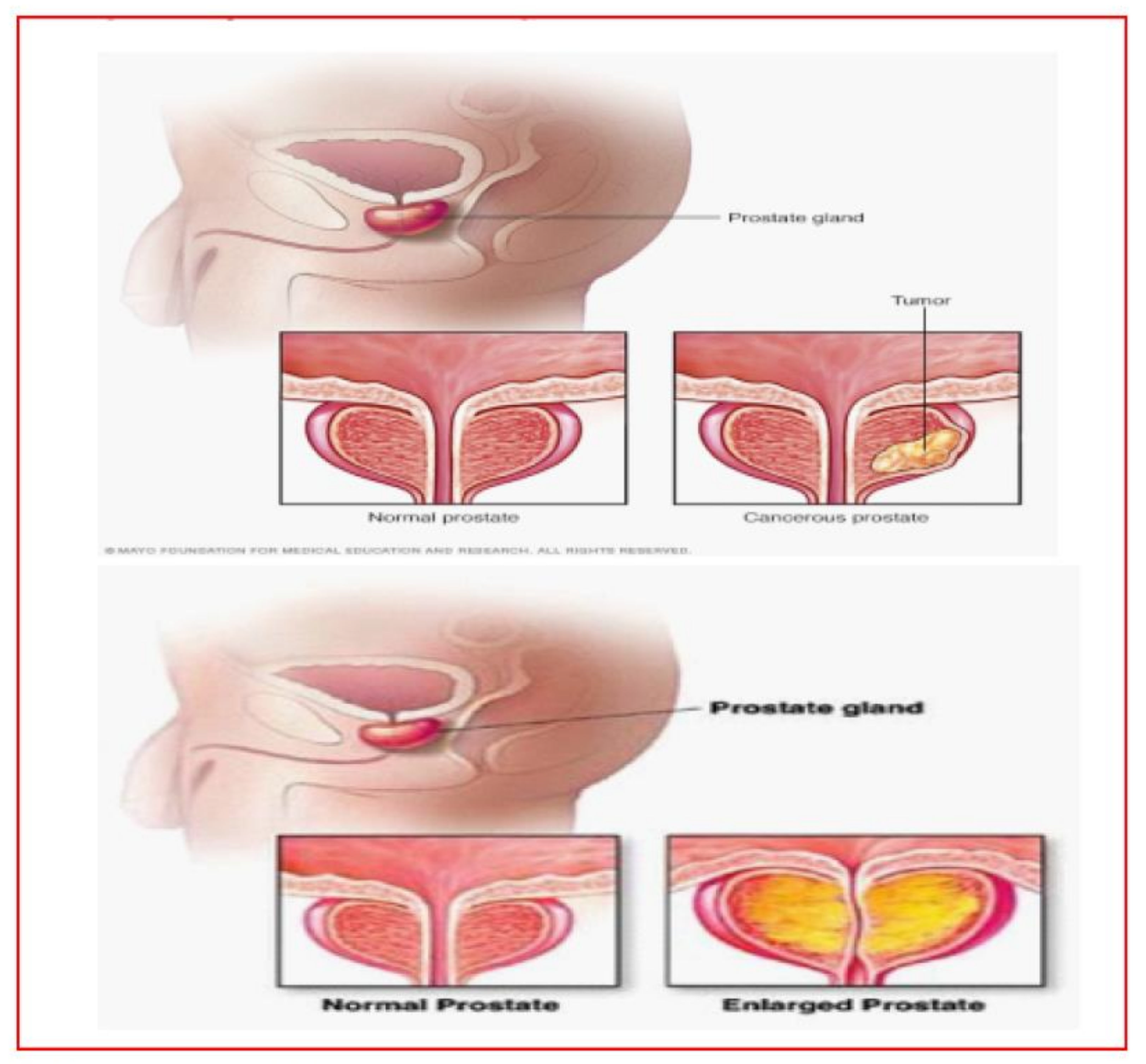
• Different stages of the prostate are shown in Figure 2.

The corresponding PC risk grades of Table 2 and Table 4 are given in

Table 5. The PC risk grades.

Risk Grades	${\mathit{S}}_1$: PSA (ng/mL)	${\mathit{S}}_2$: Gleason Score	${\mathit{S}}_3$: Clinical Staging ${\mathit{T}}_2$
${\mathbb{R}}_1(Small-risk)$	$[2,9],[2.4,4.0],[2.5,3.5]$	$[2,4],[3,5],[0,2]$	$[0,3],[1,4],[4,6]$
${\mathbb{R}}_2(Fair-risk)$	$[10,20],[4.0,10],[3.5,4.5]$	$[5,6],[6,8],[3,5]$	$[4,6],[5,7],[6,7]$
${\mathbb{R}}_3(Large-risk)$	$[21,50],[10,20],[4.5,6.5]$	$[7,10],[8,10],[6,10]$	$[7,10],[8,10],[7,10]$

.

The risk grades of PC from Table 5, NCHFN normalized transformation using the following formula:

$${\Psi }_{jk}=\left\{\begin{array}{c}{[{\alpha }_{jk}/max\left(n_{jk}\right),n_{jk}/max\left(n_{jk}\right)]}_T,{[r_{jk}/max\left(r_{jk}\right),r_{jk}/max\left(r_{jk}\right)]}_I\\ {\gamma }_{jk}/max\left(m_{jk}\right),m_{jk}/max\left(m_{jk}\right){]}_F,\\ \left({\alpha }_{jk}/max\left(n_{jk}\right)+n_{jk}/max\left(n_{jk}\right)\right)/2,(r_{jk}/max\left(r_{jk}\right)+r_{jk}/max\left(r_{jk}\right))/2,\\ ({\gamma }_{jk}/max\left(m_{jk}\right)+m_{jk}/max\left(m_{jk}\right))/2\end{array}\right\}$$

(9)

As ${\Psi }_{jk}$ is the normalized CHFNs which represent information (three outlines) of $j=1,2,3$ and $k=1,2,3$, of the risk grades of PC in

Table 6. Similarity measure values and risk evaluation grades of the 10 PC patients.

Risk Grades	${\mathit{S}}_1$	${\mathit{S}}_2$	${\mathit{S}}_3$
$R_1$(Small-risk)	$〈\begin{array}{c}<[0.04,0.18],\\ [0.12,0.2]\\ [0.38,0.54]\\ 0.11,0.16,0.46>\end{array}〉$	$〈\begin{array}{c}<[0.2,0.4],\\ [0.3,0.5]\\ [0.0,0.2]\\ \hfill 0.30,0.4,0.1>\end{array}〉$	$〈\begin{array}{c}<[0.0,0.3],\\ [0.1,0.4]\\ [0.4,0.6]\\ \hfill 0.15,0.25,0.5>\end{array}〉$
$R_2$(Fair-risk)	$〈\begin{array}{c}<[0.2,0.4],\\ [0.2,0.5]\\ [0.54,0.69]\\ \hfill 0.30,0.35,0.61>\end{array}〉$	$〈\begin{array}{c}<[0.5,0.6],\\ [0.6,0.8]\\ [0.3,0.5]\\ \hfill 0.55,0.7,0.4>\end{array}〉$	$〈\begin{array}{c}<[0.4,0.6],\\ [0.5,0.7]\\ [0.6,0.7]\\ \hfill 0.5,0.6,0.65>\end{array}〉$
$R_3$(Large-risk)	$〈\begin{array}{c}<[0.42,1],\\ [0.5,1]\\ [0.69,1]\\ 0.71,0.75,0.84>\end{array}〉$	$〈\begin{array}{c}<[0.7,1],\\ [0.8,1]\\ [0.6,1]\\ \hfill 0.85,0.9,0.8>\end{array}〉$	$〈\begin{array}{c}<[0.7,1],\\ [0.8,1]\\ [0.7,1]\\ \hfill 0.58,0.9,0.58>\end{array}〉$

.

The PC of risk grades of Table 6 can be expressed as the following NCHFSs:

$$\begin{array}{c}\hfill \begin{array}{c}\hfill {\mathbb{R}}_1=\left\{〈\begin{array}{c}<S_1,[0.04,0.18],\\ [0.12,0.2],\\ [0.38,0.54],\\ 0.11,0.16,0.46>\end{array}〉,〈\begin{array}{c}<S_2,[0.2,0.4],\\ [0.3,0.5],\\ [0.0,0.2],\\ \hfill 0.30,0.4,0.1>\end{array}〉,〈\begin{array}{c}<S_3,[0.0,0.3],\\ [0.1,0.4],\\ [0.4,0.6],\\ \hfill 0.15,0.25,0.5>\end{array}〉\right\}\end{array}\\ \hfill {\mathbb{R}}_2=\left\{〈\begin{array}{c}<S_1,[0.2,0.4],\\ [0.2,0.5],\\ [0.54,0.69],\\ \hfill 0.30,0.35,0.61>\end{array}〉,〈\begin{array}{c}<S_2,[0.5,0.6],\\ [0.6,0.8],\\ [0.3,0.5],\\ \hfill 0.55,0.7,0.4>\end{array}〉,〈\begin{array}{c}<S_3,[0.4,0.6],\\ [0.5,0.7],\\ [0.6,0.7],\\ \hfill 0.5,0.6,0.65>\end{array}〉\right\}\\ \hfill {\mathbb{R}}_3=\left\{〈\begin{array}{c}<S_1,[0.42,1],\\ [0.5,1],\\ [0.69,1],\\ 0.71,0.75,0.84>\end{array}〉,〈\begin{array}{c}<S_2,[0.7,1],\\ [0.8,1],\\ [0.6,1],\\ \hfill 0.85,0.9,0.8>\end{array}〉,〈\begin{array}{c}<S_3,[0.4,0.6],\\ [0.5,0.7],\\ [0.6,0.7],\\ \hfill 0.5,0.6,0.65>\end{array}〉\right\}\end{array}$$

Suppose that, for PC patients, the risk estimations of the T2 staging, Gleason score, and PSA level are provided by a physician group as per Table 3, Table 4 and Table 5. Therefore, based on collecting neutrosophic and cubic with the hesitant fuzzy set, the p patients’ estimation in order of PC in the form of NCHFSs can be described as

$$\begin{array}{ccc}\hfill H_i& =& \hfill \left(\begin{array}{c}<(S_{i1},[r_{i1}^{*},r_{i1}^{**}],[r_{i1}^{*},r_{i1}^{**}],[m_{i1}^{*},m_{i1}^{**}],\\ \{{(r_{i1}^1,r_{i1}^2,r_{i1}^3,\dots .,r_{i1}^{S_i})}_T,\\ {(r_{i1}^1,r_{i1}^2,r_{i1}^3,\dots ,r_{i1}^{S_i})}_I,\\ {(m_{i1}^1,m_{i1}^2,m_{i1}^3,\dots ,m_{i1}^{S_i})}_F\}>,\\ <(S_{i2},[r_{i2}^{*},r_{i2}^{**}],[r_{i2}^{*},r_{i2}^{**}],[m_{i2}^{*},m_{i2}^{**}],\\ \{{(r_{i2}^1,r_{i2}^2,r_{i2}^3,\dots .,r_{i2}^{S_i})}_T,\\ {(r_{i2}^1,r_{i2}^2,r_{i2}^3,\dots ,r_{i2}^{S_i})}_I,\\ {(m_{i2}^1,m_{i2}^2,m_{i1}^3,\dots ,m_{i1}^{S_i})}_F\}>,\\ <(S_{i3},[r_{i3}^{*},r_{i3}^{**}],[r_{i3}^{*},r_{i3}^{**}],[m_{i3}^{*},m_{i3}^{**}],\\ \{{(r_{i3}^1,r_{i3}^2,r_{i3}^3,\dots .,r_{i3}^{S_i})}_T,\\ {(r_{i3}^1,r_{i3}^2,r_{i3}^3,\dots ,r_{i3}^{S_i})}_I,\\ {(m_{i3}^1,m_{i3}^2,m_{i3}^3,\dots ,m_{i3}^{S_i})}_F\}>,\end{array}\right)\hfill \\ \hfill (i& =& 1,2,3,\dots ,q)\hfill \end{array}$$

(10)

The similarity measure is identified as a mathematical tool to express identification. In reality, PC risk-grades estimation also expresses difficulty value. In this regard, to obtain proper risk grade estimation in the context of PC patients $H_i$, the similarity measure $S_{{}_{{}_{\omega }}}(H_i,R_j)$ values for $\alpha =1$ or 2, for $i=1,2,3,\dots ,p$ is a prostate cancer patients and for $j=1,2,3$ is the risk criteria. Then, similarity measures can be determined by the following method:

$$S_{{}_{{}_{\omega }}}(H_i,R_j)=1-{\left\{\sum _{k=1}^m{\displaystyle \frac{{\omega }_k}{(S_k+2)}}\left(\begin{array}{c}{\left|r_{ik}^{*}-r_{jk}^{*}\right|}_T^{\alpha }+{\left|r_{ik}^{**}-r_{jk}^{**}\right|}_T^{\alpha }+{\left|r_{ik}^{*}{-}_{jk}^{*}\right|}_I^{\alpha }+\\ {\left|r_{ik}^{**}{-}_{jk}^{**}\right|}_I^{\alpha }+\\ {\left|m_{ik}^{*}-m_{jk}^{*}\right|}_F^{\alpha }+{\left|m_{ik}^{**}-m_{jk}^{**}\right|}_F^{\alpha }+\\ {\left|r_{ik}^1-r_{jk}^1\right|}_T^a+{\left|r_{ik}^2-r_{jk}^2\right|}_T^a+{\left|r_{ik}^3-r_{jk}^3\right|}_T^a+,\dots ,\\ {\left|r_{ik}^{S_k}-r_{jk}^{S_k}\right|}_T^a+\\ {\left|r_{ik}^1-r_{jk}^1\right|}_I^a+{\left|r_{ik}^2-r_{jk}^2\right|}_I^a+{\left|r_{ik}^3-r_{jk}^3\right|}_I^a+,\dots ,\\ {\left|r_{ik}^{S_k}-r_{jk}^{S_k}\right|}_I^a+\\ {\left|m_{ik}^1-m_{jk}^1\right|}_F^a+{\left|m_{ik}^2-m_{jk}^2\right|}_F^a+{\left|m_{ik}^3-m_{jk}^3\right|}_F^a+,\dots ,\\ {\left|m_{ik}^{S_k}-m_{jk}^{S_k}\right|}_F^a\end{array}\right)\right\}}^{\frac{1}{\alpha }}$$

(11)

The proper risk grade for $R_{j^{*}}$ of the PC patient $H_i$ is given by

$$J^{*}=arg\underset{1\le j\le 3}{max}\left\{S_{\omega }(H_i,R_j)\right\}.$$

6. Numerical Example

In this section, we give a numerical example of 10 PC patients as actual clinical cases based on Table 2, Table 3 and Table 4 by a group of three physicians. We obtain the PSA level, Gleason score, and T2 staging score for 10 PC patients, as shown in

Table 7. The risk arguments of the ten PC patients.

Patiens ${\mathit{H}}_{\mathit{i}}$	${\mathit{S}}_1$: PSA(ng/mL)	${\mathit{S}}_2$: Gleason Score	${\mathit{S}}_3$: Clinical Staging ${\mathit{T}}_2$
$H_1$	$\left\{\begin{array}{c}[11,12],[4,9],\\ [3.6,4.4]\\ \{11.1,11.3\},\\ \{4.1,4.3\},\\ \{3.7,3.9\}\end{array}\right\}$	$\left\{\begin{array}{c}[7,8],[3,4],\\ [2,4],\{7,8\}\\ \{3,4\},\{2,3\}\end{array}\right\}$	$\left\{\begin{array}{c}[6,8],[5,7],\\ [7,9],\{6,7,8\}\\ \{5,6,7\},\{7,8,9\}\end{array}\right\}$
$H_2$	$\left\{\begin{array}{c}[10,11],[7,8],\\ [3.0,4.0]\\ \{10.59,10.69\},\\ \{7.59,7.69\},\\ \{3.49,3.59\}\end{array}\right\}$	$\left\{\begin{array}{c}[5,7],[2,4],\\ [4,6],\{5,6,7\}\\ \{2,3,4\},\{4,5,6\}\end{array}\right\}$	$\left\{\begin{array}{c}[4,5],[6,7],\\ [7,8],\{4,5\}\\ \{6,7\},\{7,8\}\end{array}\right\}$
$H_3$	$\left\{\begin{array}{c}[30,32],[11,13],\\ [4.6,4.8]\\ \{30.78,30.8\},\\ \{11.78,11.8\}\\ \{4.70,4.8\}\end{array}\right\}$	$\left\{\begin{array}{c}[5,7],[2,4],\\ [4,6],\{5,6,7\}\\ \{2,3,4\},\{4,5,6\}\end{array}\right\}$	$\left\{\begin{array}{c}[4,5],[6,7],\\ [7,8],\{4,5\}\\ \{6,7\},\{7,8\}\end{array}\right\}$
$H_4$	$\left\{\begin{array}{c}[12,13],[5,7],\\ [3.55,3.6]\\ \{12.26,12.29\},\\ \{5.26,5.29\},\\ \{3.57,3.67\}\end{array}\right\}$	$\left\{\begin{array}{c}[7,8],[3,4],\\ [2,4],\{7,8\}\\ \{3,4\},\{2,3\}\end{array}\right\}$	$\left\{\begin{array}{c}[7,9],[5,7],\\ [7,9],\{7,8,9\}\\ \{5,6,7\},\{7,8,9\}\end{array}\right\}$
$H_5$	$\left\{\begin{array}{c}[46,48],[12,13],\\ [4.6,4.7]\\ \{46.68,46.76\},\\ \{12.68,12.76\},\\ \{4.61,4.64\}\end{array}\right\}$	$\left\{\begin{array}{c}[8,9],[7,8],\\ [5,6],\{8,9\}\\ \{7,8\},\{5,6\}\end{array}\right\}$	$\left\{\begin{array}{c}[9,10],[8,9],\\ [9,10],\{9,10\}\\ \{8,9\},\{9,10\}\end{array}\right\}$
$H_6$	$\left\{\begin{array}{c}[9,10],[5,7],\\ [3.6,3.8]\\ \{9.25,9.43\}\\ \{5.35,5.44\}\\ \{3.67,3.7\}\end{array}\right\}$	$\left\{\begin{array}{c}[6,7],[5,6],\\ [4,5],\{6,7\}\\ \{5,6\},\{4,5\}\end{array}\right\}$	$\left\{\begin{array}{c}[5,6],[6,7],\\ [8,9],\{5,6\}\\ \{6,7\},\{8,9\}\end{array}\right\}$
$H_7$	$\left\{\begin{array}{c}[11,12],[6,8],\\ [3.7,3.8]\\ \{11.38,11.48\},\\ \{6.11,6.48\},\\ \{3.71,3.73\}\end{array}\right\}$	$\left\{\begin{array}{c}[6,7],[5,6],\\ [4,5],\{6,7\}\\ \{5,6\},\{4,5\}\end{array}\right\}$	$\left\{\begin{array}{c}[2,3],[3,4],\\ [5,6],\{2,3\}\\ \{3,4\},\{5,6\}\end{array}\right\}$
$H_8$	$\left\{\begin{array}{c}[20,21],[10,11],\\ [4.4,4.5]\\ \{20.22,20.46\},\\ \{10.22,10.46\},\\ \{4.42,4.43\}\end{array}\right\}$	$\left\{\begin{array}{c}[7,9],[5,7],\\ [4,6],\{7,8,9\}\\ \{5,6,7\},\{4,5,6\}\end{array}\right\}$	$\left\{\begin{array}{c}[8,10],[8,9],\\ [8,10],\{8,10\}\\ \{8,9\},\{8,10\}\end{array}\right\}$
$H_9$	$\left\{\begin{array}{c}[11,12],[5,6],\\ [3.4,4.5]\\ \{11.39,11.67\},\\ \{5.39,5.67\},\\ \{3.42,3.45\}\end{array}\right\}$	$\left\{\begin{array}{c}[6,7],[5,6],\\ [4,5],\{6,7\}\\ \{5,6\},\{4,5\}\end{array}\right\}$	$\left\{\begin{array}{c}[4,6],[5,7],\\ [6,8],\{4,5,6\}\\ \{5,6,7\},\{6,7,8\}\end{array}\right\}$
$H_{10}$	$\left\{\begin{array}{c}[51,55],[15,17],\\ [4.6,4.7]\\ \{16.22,16.35\},\\ \{15.22,15.35\},\\ \{4.61,4.62\}\end{array}\right\}$	$\left\{\begin{array}{c}[7,8],[3,4],\\ [2,4],\{7,8\}\\ \{3,4\},\{2,3\}\end{array}\right\}$	$\left\{\begin{array}{c}[7,9],[5,7],\\ [7,9],\{7,8,9\}\\ \{5,6,7\},\{7,8,9\}\end{array}\right\}$

.

Ten patients’ risk arguments from Table 7 can then be changed into normalized NCHFNs, reflected in

Table 8. Ten PC patients’ risk information expressed by the normalized NCHFNs.

${\mathit{H}}_{\mathit{i}}$	${\mathit{S}}_1$	${\mathit{S}}_2$	${\mathit{S}}_3$
$H_1$	$\left\{\begin{array}{c}<[0.22,0.24],\\ [0.2,0.45],\\ [0.55,0.67],\\ \{0.222,0.226\},\\ \{0.20,0.21\},\\ \{0.57,0.6\}>\end{array}\right\}$	$\left\{\begin{array}{c}<[0.7,0.8],\\ [0.3,0.4],\\ [0.2,0.4],\\ \{0.7,0.8\},\\ \{0.3,0.4\},\\ \{0.2,0.3\}\end{array}\right\}$	$\left\{\begin{array}{c}<[0.6,0.8],\\ [0.5,0.7],\\ [0.7,0.9],\\ \{0.6,0.7,0.8\},\\ \{0.5,0.6,0.7\},\\ \{0.7,0.8,0.9\}\end{array}\right\}$
$H_2$	$\left\{\begin{array}{c}<[0.2,0.22],\\ [0.35,0.4],\\ [0.46,0.62],\\ \{0.211,0.213\},\\ \{0.38,0.39\},\\ \{0.54,0.55\}>\end{array}\right\}$	$\left\{\begin{array}{c}<[0.5,0.7],\\ [0.2,0.4],\\ [0.4,0.6],\\ \{0.5,0.6,0.7\},\\ \{0.2,0.3,0.4\},\\ \{0.4,0.5,0.6\}\end{array}\right\}$	$\left\{\begin{array}{c}<[0.4,0.5],\\ [0.6,0.7],\\ [0.7,0.8],\\ \{0.4,0.5\}\\ \{0.6,0.7\},\\ \{0.7,0.8\}\end{array}\right\}$
$H_3$	$\left\{\begin{array}{c}<[0.6,0.64],\\ [0.55,0.65],\\ [0.70,0.73],\\ \{0.615,0.616\},\\ \{0.58,0.59\},\\ \{0.72,0.72\}>\end{array}\right\}$	$\left\{\begin{array}{c}<[0.8,0.9],\\ [0.7,0.8],\\ [0.5,0.6],\\ \{0.8,0.9\},\\ \{0.7,0.8\},\\ \{0.5,0.6\}\end{array}\right\}$	$\left\{\begin{array}{c}<[0.9,1.0],\\ [0.8,0.9],\\ [0.9,1.0],\\ \{0.9,1.0\},\\ \{0.8,0.9\},\\ \{0.9,1.0\}\end{array}\right\}$
$H_4$	$\left\{\begin{array}{c}<[0.24,0.26],\\ [0.25,0.35],\\ [0.54,0.55],\\ \{0.245,0.2458\},\\ \{0.26,0.27\},\\ \{0.54,0.56\}>\end{array}\right\}$	$\left\{\begin{array}{c}<[0.7,0.8],\\ [0.3,0.4],\\ [0.2,0.4],\\ \{0.7,0.8\}\\ \{0.3,0.4\},\\ \{0.2,0.3\}\end{array}\right\}$	$\left\{\begin{array}{c}<[0.7,0.9],\\ [0.5,0.7],\\ [0.7,0.9],\\ \{0.7,0.8,0.9\},\\ \{0.5,0.6,0.7\},\\ \{0.7,0.8,0.9\}\end{array}\right\}$
$H_5$	$\left\{\begin{array}{c}<[0.92,0.96],\\ [0.6,0.65],\\ [0.70,0.72],\\ \{0.93,0.955\},\\ \{0.63,0.64\},\\ \{0.72,0.723\}>\end{array}\right\}$	$\left\{\begin{array}{c}<[0.8,0.9],\\ [0.7,0.8],\\ [0.5,0.6],\\ \{0.8,0.9\},\\ \{0.7,0.8\},\\ \{0.5,0.6\}\end{array}\right\}$	$\left\{\begin{array}{c}<[0.9,1.0],\\ [0.8,0.9],\\ [0.9,1.0],\\ \{0.9,1.0\},\\ \{0.8,0.9\},\\ \{0.8,0.9\}\end{array}\right\}$
$H_6$	$\left\{\begin{array}{c}<[0.18,0.2],\\ [0.25,0.35],\\ [0.553,0.584],\\ \{0.185,0.188\},\\ \{0.267,0.285\},\\ \{0.564,0.569\}>\end{array}\right\}$	$\left\{\begin{array}{c}<[0.6,0.7],\\ [0.5,0.6],\\ [0.4,0.5],\\ \{0.6,0.7\},\\ \{0.5,0.6\},\\ \{0.4,0.5\}\end{array}\right\}$	$\left\{\begin{array}{c}<[0.5,0.6],\\ [0.6,0.7],\\ [0.8,0.9],\\ \{0.5,0.6\},\\ \{0.6,0.7\},\\ \{0.8,0.9\}\end{array}\right\}$
$H_7$	$\left\{\begin{array}{c}<[0.22,0.24],\\ [0.3,0.4],\\ [0.569,0.584],\\ 0.227,0.229\},\\ \{0.305,0.324\},\\ \{0.570,0.573\}>\end{array}\right\}$	$\left\{\begin{array}{c}<[0.6,0.7],\\ [0.5,0.6],\\ [0.4,0.5],\\ \{0.6,0.7\},\\ \{0.5,0.6\},\\ \{0.4,0.5\}\end{array}\right\}$	$\left\{\begin{array}{c}<[0.2,0.3],\\ [0.3,0.4],\\ [0.5,0.6],\\ \{0.2,0.3\},\\ \{0.3,0.4\},\\ \{0.5,0.6\}\end{array}\right\}$
$H_8$	$\left\{\begin{array}{c}<[0.4,0.42],\\ [0.5,0.55],\\ [0.676,0.69],\\ \{0.404,0.409\},\\ \{0.51,0.523\},\\ \{0.68,0.682\}>\end{array}\right\}$	$\left\{\begin{array}{c}<[0.7,0.9],\\ [0.5,0.7],\\ [0.4,0.6],\\ \{0.7,0.8,0.9\},\\ \{0.5,0.6,0.7\},\\ \{0.4,0.5,0.6\}\end{array}\right\}$	$\left\{\begin{array}{c}<[0.8,1.0],\\ [0.8,0.9],\\ [0.8,1.0],\\ \{0.8,1.0\},\\ \{0.8,0.9\},\\ \{0.8,1.0\}\end{array}\right\}$
$H_9$	$\left\{\begin{array}{c}<[0.22,0.24],\\ [0.25,0.3],\\ [0.523,0.538],\\ \{0.229,0.233\}\\ \{0.26,0.283\},\\ \{0.526,0.530\}>\end{array}\right\}$	$\left\{\begin{array}{c}<[0.6,0.7],\\ [0.5,0.6],\\ [0.4,0.5],\\ \{0.6,0.7\}\\ \{0.5,0.6\},\\ \{0.4,0.5\}\end{array}\right\}$	$\left\{\begin{array}{c}<[0.4,0.6],\\ [0.5,0.7],\\ [0.6,0.8],\\ \{0.4,0.5,0.6\},\\ \{0.5,0.6,0.7\},\\ \{0.6,0.7,0.8\}\end{array}\right\}$
$H_{10}$	$\left\{\begin{array}{c}<[0.32,0.34],\\ [0.75,0.85],\\ [0.707,0.723],\\ \{0.324,0.327\},\\ \{0.76,767\},\\ \{0.709,0.710\}>\end{array}\right\}$	$\left\{\begin{array}{c}<[0.7,0.8],\\ [0.3,0.4],\\ [0.2,0.4],\\ \{0.7,0.8\}\\ \{0.3,0.4\},\\ \{0.2,0.3\}\end{array}\right\}$	$\left\{\begin{array}{c}<[0.7,0.9],\\ [0.5,0.7],\\ [0.7,0.9],\\ \{0.7,0.8,0.9\},\\ \{0.5,0.6,0.7\},\\ \{0.7,0.8,0.9\}\end{array}\right\}$

.

Then, the risk information of the 10 PC patients in Table 8 can be expressed as the following NCHFSs:

$$\begin{array}{c}\hfill H_1=\left\{\begin{array}{c}<S_1,[0.22,0.24],\\ [0.2,0.45],\\ [0.55,0.67],\\ \{0.222,0.226\},\\ \{0.20,0.21\},\\ \{0.57,0.6\}>\end{array}\right\},\left\{\begin{array}{c}<S_2,[0.7,0.8],\\ [0.3,0.4],\\ [0.2,0.4],\\ \{0.7,0.8\},\\ \{0.3,0.4\},\\ \{0.2,0.3\}\end{array}\right\},\left\{\begin{array}{c}<S_3,[6,8],\\ [5,7],\\ [7,9],\\ \{6,7,8\},\\ \{5,6,7\},\\ \{7,8,9\}\end{array}\right\}\\ \hfill H_2=\left\{\begin{array}{c}<S_1,[0.2,0.22],\\ [0.35,0.4],\\ [0.46,0.62],\\ \{0.211,0.213\},\\ \{0.38,0.39\},\\ \{0.54,0.55\}>\end{array}\right\},\left\{\begin{array}{c}<S_2,[0.5,0.7],\\ [0.2,0.4],\\ [0.4,0.6],\\ \{0.5,0.6,0.7\},\\ \{0.2,0.3,0.4\},\\ \{0.4,0.5,0.6\}\end{array}\right\},\left\{\begin{array}{c}<S_3,[0.4,0.5],\\ [0.6,0.7],\\ [0.7,0.8],\\ \{0.4,0.5\},\\ \{0.6,0.7\},\\ \{0.7,0.8\}\end{array}\right\}\\ \hfill H_3=\left\{\begin{array}{c}<S_1,[0.6,0.64],\\ [0.55,0.65],\\ [0.70,0.73],\\ \{0.615,0.616\},\\ \{0.58,0.59\},\\ \{0.72,0.72\}>\end{array}\right\},\left\{\begin{array}{c}<S_2,[0.8,0.9],\\ [0.7,0.8],\\ [0.5,0.6],\\ \{0.8,0.9\},\\ \{0.7,0.8\},\\ \{0.5,0.6\}\end{array}\right\},\left\{\begin{array}{c}<S_3,[0.9,1.0],\\ [0.8,0.9],\\ [0.9,1.0],\\ \{0.9,1.0\},\\ \{0.8,0.9\},\\ \{0.9,1.0\}\end{array}\right\}\end{array}$$

$$\begin{array}{c}\hfill H_4=\left\{\begin{array}{c}<S_1,[0.24,0.26],\\ [0.25,0.35],\\ [0.54,0.55],\\ \{0.245,0.2458\},\\ \{0.26,0.27\},\\ \{0.54,0.56\}>\end{array}\right\},\left\{\begin{array}{c}<S_2,[0.7,0.8],\\ [0.3,0.4],\\ [0.2,0.4],\\ \{0.7,0.8\},\\ \{0.3,0.4\},\\ \{0.2,0.3\}\end{array}\right\},\left\{\begin{array}{c}<S_3,[0.7,0.9],\\ [0.5,0.7],\\ [0.7,0.9],\\ \{0.7,0.8,0.9\},\\ \{0.5,0.6,0.7\},\\ \{0.7,0.8,0.9\}\end{array}\right\}\\ \hfill H_5=\left\{\begin{array}{c}<S_1,[0.92,0.96],\\ [0.6,0.65],\\ [0.70,0.72],\\ \{0.93,0.955\},\\ \{0.63,0.64\},\\ \{0.72,0.723\}>\end{array}\right\},\left\{\begin{array}{c}<S_2,[0.8,0.9],\\ [0.7,0.8],\\ [0.5,0.6],\\ \{0.8,0.9\},\\ \{0.7,0.8\},\\ \{0.5,0.6\}\end{array}\right\},\left\{\begin{array}{c}<S_3,[0.9,1.0],\\ [0.8,0.9],\\ [0.9,1.0],\\ \{0.9,1.0\},\\ \{0.8,0.9\},\\ \{0.8,0.9\}\end{array}\right\}\\ \hfill H_6=\left\{\begin{array}{c}<S_1,[0.18,0.2],\\ [0.25,0.35],\\ [0.553,0.584],\\ \{0.185,0.188\},\\ \{0.267,0.285\},\\ \{0.564,0.569\}>\end{array}\right\},\left\{\begin{array}{c}<S_2,[0.6,0.7],\\ [0.5,0.6],\\ [0.4,0.5],\\ \{0.6,0.7\},\\ \{0.5,0.6\},\\ \{0.4,0.5\}\end{array}\right\},\left\{\begin{array}{c}<S_3,[0.5,0.6],\\ [0.6,0.7],\\ [0.8,0.9],\\ \{0.5,0.6\},\\ \{0.6,0.7\},\\ \{0.8,0.9\}\end{array}\right\}\\ \hfill H_7=\left\{\begin{array}{c}<S_1,[0.22,0.24],\\ [0.3,0.4],\\ [0.569,0.584],\\ 0.227,0.229\},\\ \{0.305,0.324\},\\ \{0.570,0.573\}>\end{array}\right\},\left\{\begin{array}{c}<S_2,[0.6,0.7],\\ [0.5,0.6],\\ [0.4,0.5],\\ \{0.6,0.7\},\\ \{0.5,0.6\},\\ \{0.4,0.5\}\end{array}\right\},\left\{\begin{array}{c}<S_3,[0.2,0.3],\\ [0.3,0.4],\\ [0.5,0.6],\\ \{0.2,0.3\},\\ \{0.3,0.4\},\\ \{0.5,0.6\}\end{array}\right\}\\ \hfill H_8=\left\{\begin{array}{c}<S_1,[0.4,0.42],\\ [0.5,0.55],\\ [0.676,0.69],\\ \{0.404,0.409\},\\ \{0.51,0.523\},\\ \{0.68,0.682\}>\end{array}\right\},\left\{\begin{array}{c}<S_2,[0.7,0.9],\\ [0.5,0.7],\\ [0.4,0.6],\\ \{0.7,0.8,0.9\},\\ \{0.5,0.6,0.7\},\\ \{0.4,0.5,0.6\}\end{array}\right\},\left\{\begin{array}{c}<S_3,[0.8,1.0],\\ [0.8,0.9],\\ [0.8,1.0],\\ \{0.8,1.0\},\\ \{0.8,0.9\},\\ \{0.8,1.0\}\end{array}\right\}\\ \hfill H_9=\left\{\begin{array}{c}<S_1,[0.22,0.24],\\ [0.25,0.3],\\ [0.523,0.538],\\ \{0.229,0.233\}\\ \{0.26,0.283\},\\ \{0.526,0.530\}>\end{array}\right\},\left\{\begin{array}{c}<S_2,[0.6,0.7],\\ [0.5,0.6],\\ [0.4,0.5],\\ \{0.6,0.7\}\\ \{0.5,0.6\},\\ \{0.4,0.5\}\end{array}\right\},\left\{\begin{array}{c}<S_3,[0.4,0.6],\\ [0.5,0.7],\\ [0.6,0.8],\\ \{0.4,0.5,0.6\},\\ \{0.5,0.6,0.7\},\\ \{0.6,0.7,0.8\}\end{array}\right\}\\ \hfill H_{10}=\left\{\begin{array}{c}<S_1,[0.32,0.34],\\ [0.75,0.85],\\ [0.707,0.723],\\ \{0.324,0.327\},\\ \{0.76,767\},\\ \{0.709,0.710\}>\end{array}\right\},\left\{\begin{array}{c}<S_2,[0.7,0.8],\\ [0.3,0.4],\\ [0.2,0.4],\\ \{0.7,0.8\}\\ \{0.3,0.4\},\\ \{0.2,0.3\}\end{array}\right\},\left\{\begin{array}{c}<S_3,[0.7,0.9],\\ [0.5,0.7],\\ [0.7,0.9],\\ \{0.7,0.8,0.9\},\\ \{0.5,0.6,0.7\},\\ \{0.7,0.8,0.9\}\end{array}\right\}\end{array}$$

Suppose the weight for each element of $S_k$ is considered as $w_k=1/3$, where $k=1,2,3$, then by using Equation (11) taking $\alpha =2$. Then, use the similarity measure $M_w(H_i,R_j)$ between the patient $H_i$ as $i=1,2,3\dots 10$ and the risk grades $R_j$ as $j=1,2,3$ and the risk evaluation grades of the 10 PC patients, which are shown in

Table 9. Similarity measure values and risk evaluation grades of the 10 PC patients.

Patients ${\mathit{H}}_{\mathit{i}}$	${\mathit{M}}_{\mathit{w}}({\mathit{H}}_{\mathit{i}},{\mathit{R}}_{\mathit{j}})$	Risk Grade Based on Table 1
$H_1$	$0.62509,0.7927,0.4592$	$R_2$
$H_2$	$0.5945,0.6789,0.6541$	$R_2$
$H_3$	$0.5643,0.3426,0.7658$	$R_3$
$H_4$	$0.3462,0.7648,0.6534$	$R_2$
$H_5$	$0.6734,0.6212,0.6754$	$R_3$
$H_6$	$0.7124,0.7531,0.3416$	$R_2$
$H_7$	$0.5732,0.6743,0.7851$	$R_2$
$H_8$	$0.3416,0.8753,0.7641$	$R_3$
$H_9$	$0.6341,0.7346,0.8763$	$R_2$
$H_{10}$	$0.7845,0.8963,0.7453$	$R_2$

.

Table 9 reflected suitable risk grade having the largest similarity measure.

7. Comparison Analysis

This section leads us towards the comparison with existing methods to estimate the quality of the proposed model. The results of

Table 10. The 10 PC patients’ overall risk evaluation grades with other existing methods [15,21].

Patients ${\mathit{H}}_{\mathit{i}}$	${\mathit{M}}_{\mathit{w}}({\mathit{H}}_{\mathit{i}},{\mathit{R}}_{\mathit{j}})$	Method-1 Risk Grades Based on NCHFS	Method-2 Risk Grades Based on CHFS [21]	Method-3 Risk Grades Based on [15]
$H_1$	$0.62509,0.7927,0.4592$	$R_2$	$R_2$	$R_2$ or $R_3$ (indeterminacy)
$H_2$	$0.5945,0.6789,0.86541$	$R_3$	$R_2$	$R_2$
$H_3$	$0.5643,0.8426,0.7658$	$R_2$	$R_3$	$R_3$
$H_4$	$0.3462,0.7648,0.6534$	$R_2$	$R_3$	$R_2$ or $R_3$ (indeterminacy)
$H_5$	$0.6734,0.6812,0.5754$	$R_2$	$R_3$	$R_3$
$H_6$	$0.7124,0.7531,0.3416$	$R_2$	$R_2$	$R_1$ or $R_2$ (indeterminacy)
$H_7$	$0.5732,0.6743,0.7851$	$R_3$	$R_2$	$R_1$ or $R_2$ (indeterminacy)
$H_8$	$0.3416,0.8753,0.641$	$R_2$	$R_3$	$R_3$
$H_9$	$0.6341,0.7346,0.8763$	$R_3$	$R_2$	$R_2$
$H_{10}$	$0.7845,0.7363,0.7453$	$R_3$	$R_2$	$R_2$ or $R_3$ (indeterminacy)

show that, if we consider the patient $H_1$, then the risk grade is identical for all three methods, with a bit of indeterminacy in method-3. If we believe patient $H_2$, the results of Table 10 show that the risk grade is $R_3$ for method-1, $R_2$ for method-2, and method-3 as shown in the following Figure 1, Figure 2, Figure 3, Figure 4 and Figure 5.

This difference exists due to the indeterminacy covered by our proposed method, which indicates the superiority of our proposed method-1. Similarly, one can see the changes in the risk grades for other patients in Table 10, and the same is shown in the graphs of the three methods.

8. Conclusions

In the present study, an innovative approach is applied for risk evaluation and potential susceptibility in patients for early prostate cancer diagnosis. A definite set of similarity measures is defined to reach deterministic results with a consequence of establishing the superiority and usefulness of this method compared to the existing processes just by the use of data from 10 patients only. The graphic comparison with other existing methods depicts the superiority of the neutrosophic fuzzy hesitant sets approach for the early diagnosis of prostate cancer. We believe that this approach will yield similarly better results if applied to investigate other forms of cancers such as kidney, bladder, lungs, etc.; however, it is part of future research in our group.

References

1. Lin, P.-H.; Liu, J.-M.; Hsu, R.-J.; Chuang, H.-C.; Chang, S.-W.; Pang, S.-T.; Chang, Y.-H.; Chuang, C.-K.; Lin, S.-K. Depression negatively impacts survival of patients with metastatic prostate cancer. Int. J. Environ. Res. Public Health 2018, 15, 2148. [Google Scholar] [CrossRef] [PubMed] [Green Version]
2. Torre, L.A.; Bray, F.; Siegel, R.L.; Ferlay, J.; Lortet-Tieulent, J.; Jemal, A. Global cancer statistics, 2012. CA Cancer J. Clin. 2015, 65, 87–108. [Google Scholar] [CrossRef] [PubMed] [Green Version]
3. Jemal, A.; Siegel, R.; Ward, E.; Murray, T.; Xu, J.; Smigal, C.; Thun, M.J. Cancer statistics, 2006. CA Cancer J. Clin. 2006, 56, 106–130. [Google Scholar] [CrossRef] [PubMed] [Green Version]
4. Carter, H.B.; Albertsen, P.C.; Barry, M.J.; Etzioni, R.; Freedland, S.J.; Greene, K.L.; Holmberg, L.; Kantoff, P.; Konety, B.R.; Murad, M.H. Early detection of prostate cancer: Aua guideline. J. Urol. 2013, 190, 419–426. [Google Scholar] [CrossRef] [Green Version]
5. Cao, K.; Arthurs, C.; Atta-ul, A.; Millar, M.; Beltran, M.; Neuhaus, J.; Horn, L.-C.; Henrique, R.; Ahmed, A.; Thrasivoulou, C. Quantitative analysis of seven new prostate cancer biomarkers and the potential future of the ‘biomarker laboratory’. Diagnostics 2018, 8, 49. [Google Scholar] [CrossRef] [Green Version]
6. Kelly, W.K.; Scher, H.I.; Mazumdar, M.; Vlamis, V.; Schwartz, M.; Fossa, S.D. Prostate-specific antigen as a measure of disease outcome in metastatic hormone-refractory prostate cancer. J. Clin. Oncol. 1993, 11, 607–615. [Google Scholar] [CrossRef] [PubMed]
7. Chan, T.Y.; Partin, A.W.; Walsh, C.P.; Epstein, J.I. Prognostic significance of Gleason score 3+4 versus Gleason score 4+3 tumor at radical prostatectomy. Urology 2000, 56, 823–827. [Google Scholar] [CrossRef]
8. Edge, S.B.; Byrd, D.R.; Compton, C.C.; Fritz, A.G.; Greene, F.L.; Trotti, A., III. AJCC Cancer Staging Manual, 7th ed.; Springer: Berlin/Heidelberg, Germany, 2010; pp. 457–468. [Google Scholar]
9. Matzkin, H.; Eber, P.; Todd, B.; van der Zwaag, R.; Soloway, M.S. Prognostic significance of changes in prostate-specific markers after endocrine treatment of stage D2 prostatic cancer. Cancer 1992, 70, 2302–2309. [Google Scholar] [CrossRef]
10. Partin, W.; Kattan, M.W.; Subong, E.N.; Walsh, P.C.; Wojno, K.J.; Oesterling, J.E.; Scardino, P.T.; Pearson, J.D. Combination of prostate-specific antigen, clinical stage, and Gleason score to predict pathological stage of localized prostate cancer. A multi-institutional update. J. Am. Med Assoc. 1997, 277, 1445–1451. [Google Scholar] [CrossRef]
11. Pisansky, T.M.; Cha, S.S.; Earle, J.D.; Durr, E.D.; Kozelsky, T.F.; Wieand, H.S.; Oesterling, J.E. Prostate-specific antigen as a pretherapy prognostic factor in patients treated with radiation therapy for clinically localized prostate cancer. J. Clin. Oncol. 1993, 11, 2158–2166. [Google Scholar] [CrossRef]
12. Ronco, A.L.; Fernandez, R. Improving Ultrasonographic Diagnosis of Prostate Cancer with Neural Networks. Ultrasound Med. Biol. 1999, 25, 729–733. [Google Scholar] [CrossRef]
13. Metlin, C.; Lee, F.; Drago, J.; Murphy, G.P.; Investigators of the American Cancer Society National Prostate Cancer Detection Project. The American Cancer Society National Prostate Cancer Detection, Project: Findings on the detection of Early Prostate Cancer in 2425 Men. Cancer 1991, 67, 2949–2958. [Google Scholar] [CrossRef]
14. Cosma, G.; McArdle, S.E.; Reeder, S.; Foulds, G.A.; Hood, S.; Khan, M.; Pockley, A.G. Identifying the presence of prostate cancer in individuals with psa levels <20ngml-1 using computational data extraction analysis of high dimensional peripheral blood flow cytometric phenotyping data. Front. Immunol. 2017, 8, 1771. [Google Scholar] [PubMed] [Green Version]
15. Ren, S.; Wang, F.; Shen, J.; Sun, Y.; Xu, W.; Lu, J.; Wei, M.; Xu, C.; Wu, C.; Zhang, Z.; et al. Long non-coding RNA metastasis associated in lung adenocarcinoma transcript 1 derived mini RNA as a novel plasma-based biomarker for diagnosing prostate cancer. Eur. J. Cancer 2013, 49, 2949–2959. [Google Scholar] [CrossRef]
16. Stamey, T.A.; Yang, N.; Hay, A.R.; McNeal, J.E.; Freiha, F.S.; Redwine, E. Prostate-specific antigen as a serum marker for adenocarcinoma of the prostate. N. Engl. J. Med. 1987, 317, 909–916. [Google Scholar] [CrossRef]
17. Saritas, I.; Allahverdi, N.; Sert, I.U. A Fuzzy Expert System Design for Diagnosis of Prostate Cancer. In Proceedings of the International Conference on Computer Systems and Technologies—CompSysTech’03, Sofia, Bulgaria, 19–20 June 2003; pp. 345–351. [Google Scholar]
18. Saritas, I.; Allahverdi, N.; Sert, U. A fuzzy approach for determination of prostate cancer. Int. J. Intell. Syst. Appl. Eng. 2013, 1, 1–7. [Google Scholar]
19. Benecchi, L. Neuro-fuzzy system for prostate cancer diagnosis. Urology 2006, 68, 357–361. [Google Scholar] [CrossRef]
20. Yuksel, S.; Dizman, T.; Yildizdan, G.; Sert, U. Application of soft sets to diagnose the prostate cancer risk. J. Inequal. Appl. 2013, 2013, 229. [Google Scholar] [CrossRef] [Green Version]
21. Fu, J.; Ye, J.; Cui, W. An evaluation method of risk grades for prostate cancer using similarity measure of cubic hesitant fuzzy sets. J. Biomed. Inform. 2018, 87, 131–137. [Google Scholar] [CrossRef]
22. Smarandache, F. Neutrosophic Logic. Neutrosophy, Neutrosophic Set, Neutrosophic Probability; Amrican Reserch Press: Rehoboth, NM, USA, 1999. [Google Scholar]
23. Ye, J. Multiple-attribute decision-making method using similarity measures of single-valued neutrosophic hesitant fuzzy sets based on least common multiple cardinality. J. Intell. Fuzzy Syst. 2018, 34, 4203–4211. [Google Scholar] [CrossRef]
24. Aslam, M.; Albassam, M. Application of Neutrosophic Logic to Evaluate Correlation between Prostate Cancer Mortality and Dietary Fat Assumption. Symmetry 2019, 11, 330. [Google Scholar] [CrossRef]
25. Wang, H.; Smarandache, F.; Zhang, Y.Q.; Sunderaman, R. Interval Neutrosophic Sets and Logic, Theory and Applications in Computing; Hexis: Phoenix, AZ, USA, 2005. [Google Scholar]
26. Thai, H.D.; Huh, J.H. Optimizing patient transportation by applying cloud computing and big data analysis. J. Supercomput. 2022, 1–30. [Google Scholar] [CrossRef]
27. Fu, J.; Ye, J.; Cui, W. The Dice measure of cubic hesitant fuzzy sets and its initial evaluation method of benign prostatic hyperplasia symptoms. Sci. Rep. 2019, 9, 60. [Google Scholar] [CrossRef] [PubMed] [Green Version]
28. Fu, J.; Ye, J. Similarity measure with indeterminate parameters regarding cubic hesitant neutrosophic numbers and its risk grade assessment approach for prostate cancer patients. Appl. Intell. 2020, 50, 2120–2131. [Google Scholar] [CrossRef]
29. Choi, W.H.; Huh, J.H. A Survey to Reduce STDs Infection in Mongolia and Big Data Virtualization Propagation. Electronics 2021, 10, 3101. [Google Scholar] [CrossRef]
30. Ho, T.; Thanh, T.D. Discovering community Interests approach to topic model with time factor andclustering methods. J. Inf. Process. Syst. 2021, 17, 163–177. [Google Scholar]
31. Kadian, R.; Kumar, S. A novel intuitionistic Renyi’s–Tsallis discriminant information measure and itsapplications in decision-making. Granul. Comput. 2021, 6, 901–913. [Google Scholar] [CrossRef]
32. Torra, V. Hesitant fuzzy sets. Int. J. Intell. Syst. 2010, 25, 529–539. [Google Scholar] [CrossRef]
33. Jun, Y.B.; Kim, C.S.; Yang, K.O. Cubic sets. Ann. Fuzzy Math. Inform. 2012, 4, 83–98. [Google Scholar]
34. Applegate, C.; Rowles, J.; Ranard, K.; Jeon, S.; Erdman, J. Soy consumption and the risk of prostate cancer: An updated systematic review and meta-analysis. Nutrients 2018, 10, 40. [Google Scholar] [CrossRef] [Green Version]
35. Seker, H.; Odeyato, M.; Petrovic, D.; Naguib, R.N.G. A Fuzzy Logic Based Method for Prognostic Decision Making in Breast and Prostate Cancers. IEEE Trans. Inf. Technol. Biomed. 2003, 7, 114–120. [Google Scholar] [CrossRef] [PubMed]
36. Torra, V.; Narukawa, Y. On hesitant fuzzy sets and decision. In Proceedings of the 18th IEEE International Conference on Fuzzy Systems, Jeju Island, Korea, 20–24 August 2009; pp. 1378–1382. [Google Scholar]
Figure 1. Gleason’s Pattern scale.
Fractalfract 06 00648 g001
Figure 2. Different stages of the prostate.
Fractalfract 06 00648 g002
Figure 3. Graphical view of risk grades based on Method-1.
Fractalfract 06 00648 g003
Figure 4. Graphical view of risk grades based on Method-2.
Fractalfract 06 00648 g004
Figure 5. Graphical view of risk grades based on Method-3.
Fractalfract 06 00648 g005