Water Detection in Satellite Images Based on Fractal Dimension

Abstract

Identification and monitoring of existing surface water bodies on the Earth are important in many scientific disciplines and for different industrial uses. This can be performed with the help of high-resolution satellite images that are processed afterwards using data-driven techniques to obtain the desired information. The objective of this study is to establish and validate a method to distinguish efficiently between water and land zones, i.e., an efficient method for surface water detection. In the context of this work, the method used for processing the high-resolution satellite images to detect surface water is based on image segmentation, using the Quadtree algorithm, and fractal dimension. The method was validated using high-resolution satellite images freely available at the OpenAerialMap website. The results show that, when the fractal dimensions of the tiles in which the image is divided after completing the segmentation phase are calculated, there is a clear threshold where water and land can be distinguished. The proposed scheme is particularly simple and computationally efficient compared with heavy artificial-intelligence-based methods, avoiding having any special requirements regarding the source images. Moreover, the average accuracy obtained in the case study developed for surface water detection was 96.03%, which suggests that the adopted method based on fractal dimension is able to detect surface water with a high level of accuracy.

1. Introduction

Identification and monitoring of different types of surface water bodies on the Earth are necessary for numerous scientific disciplines and industrial uses and are of paramount importance in sustaining all forms of lives and ecosystems. Surface water refers to water on the surface of the Earth, including wetlands, rivers, or lakes. This definition usually excludes oceans because of their enormous size and salty character, although smaller saline water bodies are normally included [1]. Potential applications and uses of identifying and monitoring surface water include sustainable agriculture, irrigation reservoirs’ monitoring, wetland inventory, watershed monitoring, river dynamics, climate change, types of climates, environment monitoring, and flood mapping [2,3,4,5,6]. In short, identification, monitoring, and assessment of present and future water resources are essential, as water information is crucial in many areas and necessary for human life.

One way to detect and monitor surface water on the Earth is through the use of high-resolution satellite images. These satellite images can be captured with the help of a variety of remote sensing technologies and devices. Some examples of remote sensing techniques used to obtain satellite images are satellite sensors, aerial photographs, or drones. The possibilities opened by remote sensing technologies and devices, especially drones, have attracted the interest of many researchers and practitioners [7,8].

It is important to remark that the trustworthiness of satellite images depends on their resolution; in other words, low quality images will not be able to provide information with added value. After all, satellite images are often snapshots generated by different algorithms that are able to determine how the raw data from sensors must be interpreted and visualized. Through platforms like Google Earth [9] and websites like OpenAerialMap [10], satellite images are becoming increasingly ubiquitous and are available to scholars and technicians. The availability of this high-resolution imagery was exploited in this research work.

High-resolution satellite images can be processed with the help of different data-driven techniques to obtain the desired information. Some of the techniques most commonly used for satellite image processing are enhancement, feature extraction, segmentation, fusion, change detection, compression, classification, and feature detection. Researchers and practitioners often categorize these techniques into four broad categories: pre-processing, transformation, correction, and classification [11,12,13,14]. Although satellite image processing can be performed using a variety of computational methods, different methods will produce different results in a number of fields of application and use cases and, consequently, the wrong selection of techniques will produce worse results for a specific application or use case. Moreover, processing satellite images is computationally intensive and can be quite complex.

In the context of this research work, satellite images will be used to detect surface water. To obtain the necessary information from the satellite images, a method based on image segmentation plus fractal dimension analysis will be used. Then, when the fractal dimensions of the tiles in which the image is divided after segmentation are calculated, there is a clear threshold where water and land can be distinguished.

Image segmentation is a process that allows breaking down a digital image into several image segments or regions of interest. This technique allows reducing the complexity of the image to make further analysis easier and has been broadly researched and exploited by scholars and practitioners [15,16,17,18]. During the segmentation process, the same label will be assigned to all pixels belonging to the same category. When a segmentation technique is used, the input can be a single region selected by a segmentation algorithm, instead of the whole image. This will reduce the processing time and computational effort. Image segmentation can be based on detecting similarity between pixels in the image to form a segment, based on a threshold (similarity), or the discontinuity of pixel intensity values of the image (discontinuity). In an image segmentation process, the objective is to identify the content of the image at the pixel level, which means that every pixel in the image belongs to a single class, contrary to, for example, image object detection, where the bounding boxes of objects can overlap [19].

A fractal is a structure where each part has the same statistical properties as a whole. In other words, fractals are complex patterns that are self-similar across different scales and, for this reason, can be thought of as never-ending patterns that can be created by repeating a simple process indefinitely. Fractals have attracted the interest of scholars and researchers [20,21,22]. One of the reasons for this is the interesting possibilities in using fractals in a variety of very different fields of application and use cases [23,24,25,26,27,28,29]. More specifically, one of the possible uses of fractals is the image compression field, where a block-based image compression technique, which detects and decodes the existing similarities between different image regions, called fractal image compression, is applied [30].

Artificial intelligence (AI) has evolved in the last decades thanks to the progress in computer science and technology [31]. Moreover, the information storage capacity has considerably increased, allowing the treatment of massive amounts of data, which is commonly known as Big Data. Nevertheless, a systematic literature review on the existing methods capable of detecting water in aerial images reveals several challenges. Delving into the world of AI, convolutional neural networks (CNNs) have proven to be an excellent tool in the fields of deep learning (DL) and machine learning (ML) [32]. CNNs are composed of a series of layers that extract features from the pixels, just as a human eye would do. However, this type of network needs to be trained by supervised learning, which means that it is necessary to indicate the object to be detected in the training images.

Moreover, sometimes, AI techniques focused on the detection of objects in images can pose difficulties that can vary depending on the field of application and the type of image or object to be detected [33]. In fact, to use AI techniques for the same objective as the method proposed in this paper, it would be necessary to count with a set of metadata in attached files, apart from the image itself. An example is a shapefile, which is a vector format that saves the location of geographic elements and attributes associated with them.

For example, in [34], a combination of clustering and an ML classifier to detect water in high resolution aerial images, obtained from Sentinel, is presented. Nevertheless, the main difficulty in the use of this model is related to the data source, as it is necessary to use pictures with the associated geoinformation metadata.

Therefore, these requirements must be considered when preparing a dataset to train and evaluate a neural network. Likewise, there are some objects that, because of their heterogeneity, are difficult to detect using AI techniques [35].

The objective of this research work is to establish and validate a method to distinguish efficiently between water and land zones, i.e., an efficient method for surface water detection, based on image segmentation plus fractal dimension analysis. More specifically, this research work uses the computational method described in [36] to directly estimate the dimension of fractals stored as digital image files. To validate this method in the context of surface water detection, an experimental study was conducted using high-resolution satellite images freely available to researchers and practitioners at the OpenAerialMap website [10]. The proposed scheme is particularly simple and computationally efficient compared with heavy-artificial intelligence-based methods, avoiding having any special requirements regarding the source images.

The remainder of the paper is organized as follows. Section 2 introduces the proposed method for surface water detection based on image segmentation plus fractal dimension analysis. Section 3 describes the case study developed where high-quality satellite images, obtained from the freely accessible OpenAerialMap website [10], were used as the source to detect surface water. The obtained results after applying the method are also presented. Finally, in Section 4, these results are discussed and interpreted.

2. Water Detection Using Quadtree Segmentation and Fractal Dimension Analysis

The proposed method can be divided into three different phases: (1) image pre-processing, (2) image segmentation, and (3) fractal dimension analysis of the images’ tiles.

Initially, the quality of the image is far more important, as it is necessary to start with a high-resolution picture that contains a considerable quantity of information. For this reason, images taken from the open-source website known as OpenAerialMap [10] were used as the source. Although the website has more than 12,000 images, 670 sensors, and 963 providers, it is necessary to apply a filter at the time of selection. The first criterion is to obtain images containing water areas, as water detection is the main purpose of this work. As previously mentioned, this study requires high-quality images, and this requirement sets the second selection criterion. Fortunately, the source has a search engine that allows filtering by resolution level; however, size and resolution vary depending on the provider. Therefore, in this work, both criteria were applied, obtaining a set of pictures with a resolution of 300 × 300 ppi and a file size of around 20 MB, depending on the image size. Because color information has a three-dimensional property, which makes processing bulkier and heavier [37], the first step consists of transforming original RGB (red, green and blue) pictures into grayscale ones.

Secondly, once the images have been pre-processed, segmentation is performed to obtain several tiles for which the fractal dimension will be calculated. In this research work, a frequently used algorithm, called Quadtree, was used [38]. A quadtree is a tree data structure commonly used to partition a two-dimensional space by recursively subdividing it into four regions. Quadtree decomposition allows subdividing an image into regions that are more homogeneous than the image itself, thus revealing information about the structure of the image. In this work, a script was developed to apply the quadtree algorithm to an input image. Firstly, the concept known as a node was implemented, which represents a spatial region, i.e., the top-left point of the image followed by its width and height. Nevertheless, to divide the input image, it is necessary to use the mean squared error of the pixels, obtaining the concept of a purity node. Then, there are two parameters that must be set to stop the recursive subdivision of the quadtree method: the contrast and the node size. On the one hand, the contrast is defined because, if there is too much contrast, it is necessary to continue dividing, while if there is too little contrast, it is better to finish the algorithm. On the other hand, the node size depends on the size and the amount of information of the image, because a middle ground is sought, i.e., if the node size is too small, the tiles are overfitted, whereas if it is too big, the tiles provide the same information as the original image. Likewise, it is necessary to emphasize the relevance of storing the coordinates of each region, specifically the upper-left and lower-right coordinates. This step is necessary to crop the grayscale picture and to obtain all of the regions for which the fractal dimension will be calculated.

Thirdly, when the image pre-processing and segmentation have been completed, the compression fractal dimension [36] of the resulting tiles can be calculated. The greater the number of regions, the longer the processing time. In order to calculate the compression fractal dimension of each tile, the following three tasks are needed: (1) image tile resizing, (2) image tile compression, and (3) sweeping for image tile size storage. Initially, the first step consists of resizing each one of the tiles, sweeping the resizing percentage from 10% to 90% with an increment of 10%. This corresponds to reducing the image size to 10%, 20%, …, and 90% of the original file size. It is worth noting that a free library, called ImageMagick [39], was used, where the resizing percentage is related to the payload. Therefore, the greater the resizing percentage, the larger the size of the file that will be obtained. Finally, the resulting number of resized images is obtained by multiplying the set of tiles by nine. When the regions have been resized, a crucial second step is performed, which consists of a process of compression, which is necessary to obtain the fractal dimension. Again, the open-source library ImageMagick [39] was used; however, in this case, it is applied to compress each one of the tiles in GZIP file format. The third step is based on a sweep where the size of the compressed tiles is stored in rows. Thus, there will be one file with nine rows for each tile, relating each row to the resizing percentage.

To understand the next steps, it is necessary to first explain the mathematical component that supports the calculation of the compression fractal dimension, as described in detail in [36]. The initial image whose fractal dimension we want to estimate requires

$$N_i=n_x{n}_y$$

(1)

symbols to be stored, one per pixel, where N is the total number of pixels; n_x and n_y are the number of pixels along the x- and y-axis, respectively; and the subindex i stands for “image”. If a file containing this set of symbols is compressed, the minimum file size

$$S=N_{i}h$$

(2)

required to store the information of the image is the entropy S of the data file, where h (bits/symbol) is the entropy rate.

We now address the effect of changing the image resolution on the file size and its entropy. As the scale s used to represent the image is varied, the number of pixels used along each axis changes linearly with s, and the total number of pixels used to represent the image varies as

$$N_i\left(s\right)=n_x{n}_y=N_0{s}^2$$

(3)

where N₀ is an arbitrary reference number. Therefore, the optimal compressed file size is

$$S\left(s\right)=N_0{s}^{2}h\left(s\right)$$

(4)

At the same time, as a fractal body, the amount of information required to represent such an object at the scaling level s is [36]

$$N_f=2^{H\left(s\right)}=N_1{s}^D$$

(5)

where N₁ is an integer, D is the fractal dimension, and H(s) is the number of bits required to represent the fractal. Therefore, the entropy of the picture file follows the scaling asymptotic

$$S\left(s\right) ~ 2^{H\left(s\right)} ~ s^D$$

(6)

and we can estimate the fractal dimension D from the sizes of the image files after compression at each resolution level s by calculating the compression dimension.

$$D_c=\underset{s \to \infty }{\lim }\frac{logS\left(s\right)}{logs}$$

(7)

The compression dimension calculation will only provide a valid estimate of the fractal dimension if the image file gives a truthful representation of the fractal object in full detail at all of the scaling levels considered. That is,

$$N_f\left(s\right)\ll N_i\left(s\right)$$

(8)

at all values of s used in the calculation. Equation (8) sets a bound on the minimum usable resolution of the image file at the beginning of the calculation and the depth of the values of s used in the estimation algorithm.

When the sizes of the compressed tiles are stored in files, linear regression is calculated for each file, sweeping the nine values. In this operation, the slope is obtained facing the logarithm of the resizing scale against the logarithm of the compressed sizes. Although the resizing scale ideally ranges from 10% to 90% [36], an exhaustive study shows that, for the tiles used, there is a turning point where the linearity disappears, indicating the violation of Equation (7). Therefore, in this research work, the scale varies between 70% and 90%, i.e., the reduced information contents in the scaled versions with resizing percentages between 60% and 10% yield meaningless data. Finally, the slope calculated for each tile corresponds to the fractal dimension of a specific tile.

To finish, when the fractal dimensions of the tiles are calculated, it is found that there is a clear threshold where surface water and land zones can be distinguished. This threshold depends on the scenario, defined as a collection of pictures captured under the same conditions, i.e., they must have the same resolution, pixel dimensions, bit depth, dynamic range, and so on. In addition, a threshold is calculated for each scenario, carrying out a loop to test the accuracy obtained with a range of thresholds, selecting the threshold that allows the best accuracy to be obtained. Likewise, this range of thresholds oscillates between the smallest and the largest fractal dimension, obtained in the first picture of each scenario.

Besides, it is necessary to clarify how the accuracy is calculated, for which it is essential to label each tile to obtain a ground truth. Likewise, the accuracy percentage is calculated by dividing the correctly classified tiles by the total number of tiles and multiplying the result by one hundred. Then, in order to validate the established threshold, this threshold is applied to another image of the same scenario and its accuracy is calculated. As the threshold varies according to the scenario, two application scenarios were established, with two images each. The first image of each scenario is used to calculate the optimal threshold, while the second image of each scenario is used to validate the previously calculated threshold. This shows that it is possible to set clear thresholds for different scenarios where surface water and land zones can be distinguished. To show the results, as previously explained, the tiles must have been labeled, thus a comparison can be made contrasting the predictions made with the fractal dimension against the true labels.

3. Results

In this work, high-quality satellite images, obtained from OpenAerialMap [10], were used to detect surface water. The results show that it is possible to set a threshold in the fractal dimension that allows differentiation between surface water and land zones.

However, it is more important to determine the accuracy, which must be studied for each picture, as the accuracy will determine the validity or not of the proposed method. Each image presents a specific accuracy; however, the average obtained in this work is 96.03%, which indicates good performance of the proposed method.

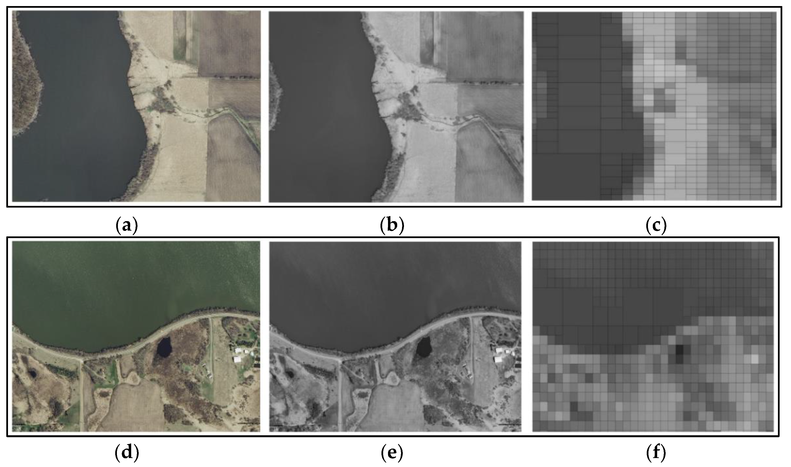
The first scenario has two different images, one to set the optimal threshold of this scenario (Figure 1a) and one to validate this threshold (Figure 1d). Next, image pre-processing was applied, converting RGB images into gray-scale ones (Figure 1b,e).

In Figure 1c–f, the segmentation performed by the Quadtree algorithm can be observed. The number of tiles depends on the size and the amount of information in the picture. In the first image, the minimum region size was set to 30 pixels, obtaining 757 tiles. Nevertheless, in the second picture, the minimum region size was set to 60 pixels owing to the dimensions, obtaining 934 tiles.

In Figure 2, a distribution histogram of the fractal dimensions of the first scenario can be observed. The x-axis shows the range in which the fractal dimensions are delimited, whereas on the y-axis, the frequency of repetition can be analyzed.

Then, in Figure 3a,b, the resizing evolution of a specific tile of the first image and the second image in the first scenario, correspondingly, can be analyzed. The first resizing corresponds to 90% and the last one corresponds to 10%; therefore, the last image contains more information.

Finally, Figure 4a,b show the results of the images of the first scenario. The accuracy of the first picture is 94.98%, whereas the second image obtains an accuracy of 96.79%. The threshold obtained on the first scenario is 1.86. As can be seen, using the threshold obtained for image 1 in image 2, an even higher accuracy is obtained, validating that the water was clearly identified for this scenario.

The second scenario is also composed of two different images, one to establish the optimal threshold of this scenario (Figure 5a) and one to validate this threshold (Figure 5d). Again, next, image pre-processing was applied, converting RGB images into gray-scale ones (Figure 5b,e).

In Figure 5c,f, the segmentation performed by the Quadtree algorithm can be observed. In the first image, the minimum region size was set to 60 pixels, obtaining 1024 tiles. In the second picture, the minimum region size was set to 30 pixels, obtaining 505 tiles. Again, the reason that the number of tiles is higher than in the first scenario is because of the amount of information contained in the image, as well as its size.

Again, Figure 6 shows a distribution histogram of the fractal dimensions of the second scenario. The x-axis shows the range in which the fractal dimensions are delimited, whereas on the y-axis, the frequency of repetition can be analyzed.

Again, in Figure 7a,b, the resizing evolution of a specific tile of the first image and the second image in the second scenario, correspondingly, can be analyzed. The first resizing corresponds to 90% and the last one corresponds to 10%; therefore, the last image contains more information.

Finally, Figure 8a,b show the results of the images of the second scenario. The accuracy of the first picture is 95.51%, whereas the accuracy of the second picture is 96.83%. The threshold obtained on the scenario is 1.90. As in the previous scenario, using the threshold obtained for image 1 in image 2, a higher accuracy is obtained, demonstrating once again that the water areas were clearly identified for this scenario too.

4. Discussion

The method proposed in this paper, based on image segmentation, performed with the Quadtree algorithm, and compression fractal dimension calculation of the tiles in which the image is divided after completing the segmentation phase, in order to detect surface water bodies on Earth, is particularly simple, especially when compared with the complex techniques used in AI. It is also remarkable that this method does not have any special requirements regarding the data source, which is a great advantage, because only the image is needed, but no geoinformation metadata are required. Moreover, from a computational point of view, the proposed method, based on the computational scheme described in [36] to directly estimate the dimension of fractals stored as digital image files, involves lighter tasks than the training and related tasks of artificial neural networks. Moreover, the average accuracy obtained in the work developed for surface water detection was 96.03%, which suggests that the fractal dimension is quite useful to detect surface water with a high level of accuracy.