Modeling and Calibration for Some Stochastic Differential Models

Abstract

In many scientific fields, the dynamics of the system are often known, and the main challenge is to estimate the parameters that model the behavior of the system. The question then arises whether one can use experimental measurements of the system response to derive the parameters? This problem has been addressed in many papers that focus mainly on data from a deterministic model, but few efforts have been made to use stochastic data instead. In this paper, we address this problem using the following procedure: first, we build the probabilistic stochastic differential models using a natural extension of the commonly used deterministic models. Then, we use the data from the stochastic models to estimate the model parameters by solving a nonlinear regression problem. Since the stochastic solutions are not differentiable, we use the well-known Nelder–Mead algorithm. Our numerical results show that the fitting procedure is able to obtain good estimates of the parameters requiring only a few sample data.

1. Introduction

The most common approach to studying many biological, ecological, or engineering systems is based on nonlinear dynamic models. One of the major challenges is the calibration of these dynamical models, also known as the parameter estimation problem, which involves finding the unknown parameters of the model that best fit a set of experimental data. Parameter estimation belongs to the class of so-called inverse problems [1], which require not only a prior assumption about the unknown parameters but also a posterior study of the determinability of the parameters. This problem has been tackled by many authors in various fields of science (see reference [2] for practical applications and numerical solutions, and reference [3] for a comprehensive review).

Parameter estimation in finite-dimensional stochastic differential equations (SDEs) has also been addressed in the literature (see [4,5,6,7]).

The classical nonlinear regression problem, which often arises in applications, concerns how to find the values of the parameters when the equations governing the system are known. The main challenge then is to use experimental results or experimental data to derive the values of the system parameters. This problem is currently being addressed by many machine learning techniques, see [8] (Cap. 9) or [9] (Cap. 7).

In this paper, we address this problem considering stochastic data, which seems to be a challenging task.

For an n-dimensional system, the stochastic differential equations (SDE) governing its dynamics are of the form

$$d\mathbf{X}=\mu (t,\mathbf{X})+\mathbf{B}(t,\mathbf{X})d\mathbf{W},$$

(1)

where $\mathbf{X}\in {\Re }^n$ is the n-dimensional state vector, $\mathbf{W}\in {\Re }^m$ refers to m independent Wiener processes, $\mu (t,\mathbf{X})\in {\Re }^n$ is the vector drift function, and $\mathbf{B}(t,\mathbf{X})\in {\Re }^{n\times m}$ is the diffusion matrix. In practice, as we will see in the following sections, these SDEs depend on a number of parameter ${\alpha }_1,\cdots ,{\alpha }_p$ whose values determine the behavior of the solutions.

The main idea now is to use the data from Equation (1) to derive the values of the parameters ${\alpha }_1,\cdots ,{\alpha }_p$. To do this, we use the least squares method, which is a common approach in regression analysis to solve over-determined systems. The error function has the form for n steps

$$E({\alpha }_1,\cdots ,{\alpha }_p)=\sum _{j=1}^n{\left({\mathbf{X}}_d\left(t_j\right)-\frac{1}{nrum}\sum _{i=1}^{nrum}{\mathbf{X}}_{j,i}\right)}^2,$$

(2)

where $\left\{{\mathbf{X}}_d\left(t_j\right)\right\}$ are the solutions of the deterministic part computed with the "ode45" command from Matlab; these solutions are obviously dependent on the values of the parameters, and $\left\{{\mathbf{X}}_{j,i}\right\}$ is the stochastic solution ant time $t_j$ for the $ith$ run or trial using the classical numerical Euler–Maruyama method (we refer to [10,11] and more recently [12] for an overview of numerical solutions of SDEs).

Since we are dealing with a nonlinear optimization problem involving stochastic data, we used the Nelder–Mead algorithm [13,14] (p. 325) or [15] (p. 368) to minimize Equation (2), which proved to be more suitable in these cases.

On the order hand, from the two papers [16,17], in our opinion, it would seem that the most natural extension of moving from a deterministic model to a stochastic model would be to use probabilities instead of simply adding white noise. In these stochastic models that we studied in this paper, which we refer to as probabilistic models, we use tables of probabilities of change and compute the means and variances following [18].

This article is structured as follows. In Section 2 we consider a classical predator–prey model, in Section 3 an epidemic model, and finally in Section 4 a chemical-reaction model. For these three models, we first build the stochastic model and then try to calibrate the parameters using the Nelder–Mead algorithm and solve the deterministic part using the "ODE45" Matlab solver. Finally, in Section 5 we analyze the numerical results and draw the main conclusions and possible future research.

2. A Predator–Prey Model

In this first model, we study the well-known Lotka–Volterra predator–prey system, where the preys are rabbits, which have an infinite food supply, and the predators are foxes. This example was previously studied in [17,19], assuming that the changes and their probabilities are those given in Table 1.

Table 1. Population changes and their probabilities.

Change	Probability
$\Delta {\mathbf{X}}^{\left(1\right)}={(1,0)}^T$	$p_1=\beta R\Delta t$
$\Delta {\mathbf{X}}^{\left(2\right)}={(0,1)}^T$	$p_2=\alpha RF\Delta t$
$\Delta {\mathbf{X}}^{\left(3\right)}={(-1,0)}^T$	$p_3=\alpha RF\Delta t$
$\Delta {\mathbf{X}}^{\left(4\right)}={(0,-1)}^T$	$p_4=F\Delta t$

That is, given the parameter $\alpha >0$, the fox encounters the rabbit with a probability proportional to the product of their numbers, and $\beta >0$ is a coefficient for the reproduction of the rabbits.

Fixing $\mathbf{X}\left(t\right)$ at time t, we calculate the expected change for $\mathbf{X}={(R,F)}^T$

$$\mathrm{E}(\Delta \mathbf{X})=\sum _{j=1}^4{p}_j\Delta {\mathbf{X}}^{\left(j\right)}=\left(\begin{array}{c}R(\beta -\alpha F)\\ F(\alpha R-1)\end{array}\right)\Delta t,$$

(3)

and the covariance matrix

$$\mathrm{E}(\Delta \mathbf{X}{(\Delta \mathbf{X})}^T)=\sum _{j=1}^4{p}_j(\Delta {\mathbf{X}}^{\left(j\right)}){(\Delta {\mathbf{X}}^{\left(j\right)})}^T=\left(\begin{array}{cc}R(\beta +\alpha F)& 0\\ 0& F(\alpha R+1)\end{array}\right)\Delta t,$$

(4)

results in the following SDE system:

$$\left\{\begin{array}{c}dR=R(\beta -\alpha F)dt+\sqrt{R(\beta +\alpha F)}d{W}_1\left(t\right),\\ dF=F(\alpha R-1)dt+\sqrt{F(\alpha R+1)}d{W}_2\left(t\right).\end{array}\right.$$

(5)

where $W_1$ and $W_2$ are two independent Wiener processes.

Fitting Model to Data

In this example, the error function is

$$E(\alpha ,\beta )=\sum _{j=1}^n\left(|R\left(t_j\right)-R_j{|}^2+{|F\left(t_j\right)-F_j|}^2\right),$$

(6)

where $R_j$ and $F_j$ are the stochastic data averaged over a given number of trials (nrum) using the Euler–Maruyama method. $R\left(t\right)$ and $F\left(t\right)$ are the solution of the deterministic equations. The goal is then to find the values of $\alpha$ and $\beta$ using a fitting method. To evaluate the error function for a given solution $(\alpha ,\beta )$, the deterministic part of the system (5) is first solved numerically. This solution is then used to construct a clamped cubic spline interpolation function that can be evaluated to obtain values for R and F at the various $t_j$’s appearing in the error function.

Table 2 reports the average values of the parameters obtaind using the Nelder–Mead algorithm as a function of the number of trials and the number of iteration steps. The initial point is $R\left(0\right)=150$, $F\left(0\right)=50$, and the parameters are $\alpha =0.05$, $\beta =2$ and $0\le t\le 5$.

Table 2. Estimated average values of the parameters obtained using the Nelder–Mead algorithm as a function of the number of trials and the number of iteration steps for $\alpha =0.05,\beta =2$, and $0\le t\le 5$.

Trials	Steps	$\mathit{\alpha }$	$\mathit{\beta }$
1	59	0.04972620	1.933725
5	60	0.04924106	1.922077
10	62	0.05020194	1.929457
100	61	0.05099946	2.071467
1000	58	0.05018393	1.935545

Given these results, it is perhaps most surprising that our algorithm achieves good approximation of the actual parameters with just a single trial. On the other hand, we note that the performance of the algorithm is achieved with few iterations, regardless of the number of trials.

For graphical illustration, we have plotted (see Figure 1) the phase space corresponding to a stochastic simulation of the Lotka–Volterra model with the estimated parameters (red colour) and the actual parameters (blue colour). The results are shown for a single trial (left panel) and the average over 100 trials (right panel). We also plotted the average values of the parameters as a function of the number of trials (see Figure 2).

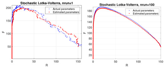
Figure 1. Predator–prey model. Phase space corresponding to a stochastic simulation of the Lotka–Volterra model using the estimated parameters (red color) compared to the actual ones (blue color). Results are shown for a single trial (left panel) and average over 100 trials (right panel).

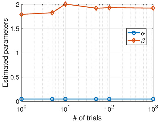
Figure 2. Predator–prey model. Average values of the parameters estimated using the Nelder–Mead algorithm as a function of the number of trials.

3. A Stochastic SIS Model with Deaths

Here, we review the main points of the SIS model with demography [20,21]. In this paper, we consider an infection model of the population where only deaths of infected individuals are considered. The changes and their first-order probabilities in the $▵t$ are those in Table 3.

Table 3. Population changes and probabilities of infection, death, and recovery of infected individuals.

Change	Propability
$\Delta {\mathbf{X}}^{\left(1\right)}={(-1,1)}^T$	$p_1=\alpha SI/(S+I)\Delta t$
$\Delta {\mathbf{X}}^{\left(2\right)}={(0,-1)}^T$	$p_2=\beta I\Delta t$
$\Delta {\mathbf{X}}^{\left(3\right)}={(1,-1)}^T$	$p_3=\gamma I\Delta t$

As in the previous example, the mean and variance were calculated according to [18] (p. 148) and using Symbolic Math Toolbox of Matlab©. The obtained stochastic model is then:

$$\begin{array}{c}\hfill d\left(\begin{array}{c}S\\ I\end{array}\right)=\left(\begin{array}{c}{\mu }_1(S,I)\\ {\mu }_2(S,I)\end{array}\right)dt+\mathbf{B}(S,I)\left(\begin{array}{c}d{W}_1\\ d{W}_2\end{array}\right),t>0,\hfill \end{array}$$

(7)

where

$${\mu }_1(S,I)=-\frac{\alpha SI}{S+I}+\gamma I,{\mu }_2(S,I)=\frac{\alpha SI}{S+I}-(\gamma +\beta )I,$$

and

$$\mathbf{B}(S,I)={\displaystyle \frac{1}{q}}\left(\begin{array}{cc}\gamma I+p+{\displaystyle \frac{\alpha SI}{S+I}}& -\gamma I-{\displaystyle \frac{\alpha SI}{S+I}}\\ -\gamma I-{\displaystyle \frac{\alpha SI}{S+I}}& \gamma I+\beta I+p+{\displaystyle \frac{\alpha SI}{S+I}}\end{array}\right),$$

with

$$p^2=\gamma \beta I^2+\frac{\alpha \beta S{I}^2}{S+I}\mathrm{and}{q}^2=2\gamma I+\beta I+2p+\frac{2\alpha SI}{S+I}.$$

The deterministic version of this model is given by

$$\begin{array}{ccc}\hfill \frac{dS}{dt}& =& \hfill -\frac{\alpha SI}{S+I}+\gamma I,\hfill \\ \hfill \frac{dI}{dt}& =& \hfill \frac{\alpha SI}{S+I}-(\gamma +\beta )I.\hfill \end{array}$$

(8)

The asymptotic behavior of this system depends on the basic reproduction number $R=\alpha /(\gamma +\beta )$, and according to [22], this model reaches a disease-free equilibrium when $R\le 1$. In this paper, we consider the particular case with the parameters $\alpha =0.0429$, $\beta =0.00137$, and $\gamma =0.02011$, such that $R=1.9972>1$.

Fitting Model to Data

For this model, the error function is given as a function of three parameters,

$$E(\alpha ,\gamma ,\beta )=\sum _{j=1}^n\left\{\right|S\left(t_j\right)-S_j{|}^2+|I\left(t_j\right)-I_j{|}^2\},$$

(9)

where $S_j$ and $I_j$ refer to the average stochastic data over a number of trials using the Euler–Maruyama method, while $S\left(t\right)$ and $I\left(t\right)$ are the solution of the deterministic equations.

The results given in Table 4 were obtained with initial conditions $R\left(0\right)=150,F\left(0\right)=50$, and parameters $\alpha =0.0429,\gamma =0.02011,\beta =0.00137$, and $0\le t\le 300$. The phase space corresponding to a stochastic simulation of the SIS model with the estimated parameters (red colour) and the actual parameters (blue colour) is shown in Figure 3.

Table 4. Average values of the parameters estimated using the Nelder–Mead algorithm as a function of the number of trials. The number of required iteration steps to achieve these estimated parameters is also reported. The values of actual parameters are $\alpha =0.0429,\gamma =0.02011,\beta =0.00137$.

# Trials	# Steps	$\mathit{\alpha }$	$\mathit{\gamma }$	$\mathit{\beta }$
1	47	0.0823	0.0375	0.0057
5	51	0.0453	0.0188	0.0019
10	43	0.0425	0.0156	0.0017
50	47	0.0387	0.0159	0.0014
100	48	0.0345	0.0126	0.0013
1000	46	0.0390	0.0155	0.0013

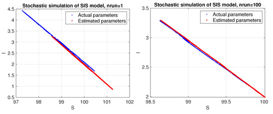
Figure 3. SIS model. Phase space corresponding to a stochastic simulation using the estimated parameters (red color) compared to the actual ones (blue color). Results are shown for a single trial (left panel) and average over 100 trials (right panel).

Unlike the Lotka–Volterra model, the SIS model appears to be more sensitive to random data and requires averaging stochastic data over a sufficient number of trials to obtain good estimates for the parameters. As can be seen in Figure 4, the estimated parameters converge toward the actual values as the number of trials increases.

Figure 4. Average values of the parameters estimated using the Nelder–Mead algorithm as a function of the number of trials.

4. A Chemical-Reaction Model

In our third experiment, we consider the Michaelis–Menten model for chemical reactions. In this model, we consider a system with four nonnegative variables: $S_1\left(t\right)$, $S_2\left(t\right)$, $S_3\left(t\right)$, and $S_4\left(t\right)$, which refer to the concentrations of substrate, enzyme, complex, and product, respectively. These chemical reactions are described in the following form:

$$\begin{array}{ccc}\hfill S_1+S_2& \stackrel{k_1}{⟶}& S_3,\hfill \\ \hfill S_3& \stackrel{k_2}{⟶}& \hfill S_1+S_2,\hfill \\ \hfill S_3& \stackrel{k_3}{⟶}& \hfill S_4+S_2.\hfill \end{array}$$

where $k_1,k_2$, and $k_3$ are the reaction constants.

To construct the stochastic system, we define the new variables

$$X_i\left(t\right)=S_i\left(t\right)·{\mathfrak{n}}_A·\mathrm{Vol},i=1,\cdots ,4,$$

(10)

where ${\mathfrak{n}}_A\approx 6.023\times {10}^{23}$ is the Avogadro’s number. The possible random changes at each time step $▵t$ are given in Table 5 where

$$a_1\left(t\right)=k_1{X}_1\left(t\right)X_2\left(t\right),a_2\left(t\right)=k_2{X}_3\left(t\right),a_3\left(t\right)=k_3{X}_3\left(t\right).$$

(11)

Table 5. Possible change in $\mathbf{X}={(X_1,X_2,X_3,X_4)}^T$ and their probabilities.

Change	Propability
$\Delta {\mathbf{X}}^{\left(1\right)}={(-1,-1,1,0)}^T$	$p_1=a_1\left(t\right)\Delta t$
$\Delta {\mathbf{X}}^{\left(2\right)}={(1,1,-1,0)}^T$	$p_2=a_2\left(t\right)\Delta t$
$\Delta {\mathbf{X}}^{\left(3\right)}={(0,1,-1,1)}^T$	$p_3=a_3\left(t\right)\Delta t$

In this paper, we set the values of the parameters as given in [23]. The molecular data corresponding to concentrations within a volume of $Vol={10}^{-15}$ liters are given as follows:

$$X_1\left(0\right)=5\times {10}^{-7}(n_A\times Vol),X_2\left(0\right)=2\times {10}^{-7}(n_A\times Vol),X_3\left(0\right)=0,X_4\left(0\right)=0,$$

$$k_1=\frac{{10}^6}{(n_A\times Vol)},k_2={10}^{-4},k_3={10}^{-1},$$

Following [24], we obtain a stochastic differential system with four independent Brownian motions and show that is equivalent to the chemical Langevin model (see e.g. [25,26,27] or [28]), i.e.,

$$d\mathbf{X}\left(t\right)=\sum _{j=1}^3{\mathbf{v}}_j{a}_j\left(\mathbf{X}\left(t\right)\right)+\sum _{j=1}^3{\mathbf{v}}_j\sqrt{a_j\left(\mathbf{X}\left(t\right)\right)}d{W}_j\left(t\right),$$

(12)

with only three independent Brownian motions and the state change vectors

$${\mathbf{v}}_1=\left(\begin{array}{c}\hfill -1\\ \hfill -1\\ \hfill 1\\ \hfill 0\end{array}\right),{\mathbf{v}}_2=\left(\begin{array}{c}\hfill 1\\ \hfill 1\\ \hfill -1\\ \hfill 0\end{array}\right),{\mathbf{v}}_3=\left(\begin{array}{c}\hfill 0\\ \hfill 1\\ \hfill -1\\ \hfill 1\end{array}\right),$$

we will use this second model (12) because it is easier to simulate.

Fitting Model to Data

Following the same procedure as in the previous two cases, the error function is

$$E(k_1,k_2,k_3)=\sum _{j=1}^n\left(\sum _{i=1}^3{|X_i\left(t_j\right)-{\left(X_i\right)}_j|}^2\right),$$

(13)

where ${\left(X_i\right)}_j$ refer to the average stochastic data over a number of trials using the Euler–Maruyama method, while $X_i\left(t_j\right)$ are the solution of the deterministic equations.

The average values of the estimated parameters obtained by the Nelder–Mead algorithm as a function of the number of trials and the number of iterations are given in Table 6.

Table 6. Average values of the parameters obtained using the Nelder–Mead algorithm as a function of the number of trials and the number of iteration steps. The original values of parameters are $k_1=0.0017$, $k_2=0.0001$, and $k_3=0.1$.

# Trials	# Iteration	${\mathit{k}}_1$	${\mathit{k}}_2$	${\mathit{k}}_3$
1	41	0.0014	0.0001	0.1134
5	42	0.0016	0.0002	0.1074
10	44	0.0016	0.0004	0.1179
50	41	0.0016	0.0002	0.1141
100	42	0.0016	0.0002	0.1131
1000	37	0.0016	0.0002	0.1146

In this case, the achieved results are less dependent on the level of randomness of the data and show a stable behavior as can be seen in Figure 5. We also plotted the phase space corresponding to a stochastic simulation of the Higham chemical model using the estimated parameters (red color) compared to the actual parameters (blue color). The results are shown in Figure 6 for a single trial (left panel) and the average over 100 trials (right panel).

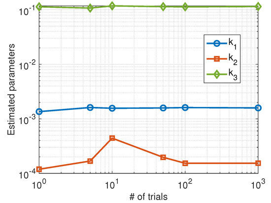
Figure 5. Average values of the parameters estimated using the Nelder–Mead algorithm as a function of the number of trials.

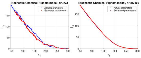
Figure 6. Phase space corresponding to a stochastic simulation of the Higham chemical model using the estimated parameters (red color) compared to the actual parameters (blue color). The results are shown for a single trial (left panel) and average over 100 trials (right panel).

5. Conclusions

The main conclusion we draw from our research is that the fitting procedure used in this paper to determine parameters from data is valid even when the data come from stochastic models. The approach has been successfully tested on three stochastic models from different domains. Moreover, in all cases it seems that few samples are sufficient to obtain good estimates for the parameters.

We wonder if this procedure will be applicable in general SDE. The error function (2) for $nrum$ large can be written as

$$E({\alpha }_1,\cdots ,{\alpha }_p)=\sum _{j=1}^n{\left({\mathbf{X}}_d\left(t_j\right)-\mathbf{E}\left({\mathbf{X}}_j\right)\right)}^2,$$

(14)

assuming that the mean of the stochastic solution equals the deterministic solution. In particular when the drift is linear is true [12] (p. 66) but is false when the SDE is nonlinear, for example, the SDE

$$dX\left(t\right)=-0.25X^3\left(t\right)+0.5X^2\left(t\right)dW\left(t\right),X\left(0\right)=0.5,$$

(15)

the mean satisfies $\mathbf{E}\left(X\right(t\left)\right)=0.5-0.03125t$, while the solution of the deterministic part is ${\displaystyle X_d\left(t\right)=\frac{2}{\sqrt{2t+16}}}$.

However, for our models, the procedure achieves excellent results. Perhaps the previous hypothesis applies to our models; we do not know at the moment.

Consistent with the work and our preliminary studies, techniques developed in recent years [29,30] for discovering nonlinear dynamical equations from data, without making assumptions about the underlying equations of motion, appear to work with stochastic data and provide promising results. In the future, we plan to investigate various differential models and attempt to discover their dynamics using data from the corresponding stochastic models.

On the other hand, since derivatives of a non-integer order [31] are a natural generalization of the ordinary differentiation of integer order, mathematical models using fractional-order differential equations have proven to be a suitable tool to study and understand temporal memory and intrinsic dissipative processes in many physical and biological systems. To our knowledge, however, there have been few attempts to estimate the parameters of fractional-order stochastic systems. In [32], the authors investigated estimation problems for difusion processes satisfying SDEs driven by mixed fractional Brownian motion. In the future, we hope to be able to extend the approach presented in this paper to consider fractional-order SDEs.

References

- Clermont, G.; Zenker, S. The inverse problem in mathematical biology. Math. Biosci. 2015, 260, 11–15. [Google Scholar] [CrossRef] [PubMed]
- Schittkowski, K. Numerical Data Fitting in Dynamical Systems: A Practical Introduction with Applications and Software; Springer Science & Business Media: Berlin/Heidelberg, Germany, 2002; Volume 77. [Google Scholar]
- McGoff, K.; Mukherjee, S.; Pillai, N. Statistical inference for dynamical systems: A review. Stat. Surv. 2012, 9, 209–252. [Google Scholar] [CrossRef]
- Liu, Q.A.; Varshney, D.; McAuley, K.B. Parameter and uncertainty estimation in stochastic differential equation models with multi-rate data and nonstationary disturbances. Chem. Eng. Res. Des. 2022, 183, 118–133. [Google Scholar] [CrossRef]
- Nielsen, J.N.; Madsen, H.; Young, P.C. Parameter estimation in stochastic differential equations: An overview. Annu. Rev. Control. 2000, 24, 83–94. [Google Scholar] [CrossRef]
- Bishwal, J.P. Bayes and Sequential Estimation in Stochastic PDEs. In Parameter Estimation in Stochastic Differential Equations; Springer: Berlin/Heidelberg, Germany, 2008; pp. 79–97. [Google Scholar]
- Bishwal, J.P. Maximum Likelihood Estimation in Fractional Diffusions. In Parameter Estimation in Stochastic Differential Equations; Springer: Berlin/Heidelberg, Germany, 2008; pp. 99–122. [Google Scholar]
- Deisenroth, M.; Faisal, A.A.; Ong, C.S. Mathematics for Machine Learning. Available online: https://mml-book.github.io/book/mml-book.pdf (accessed on 2 November 2022).
- Murphy, L. Machine Learning. A Probabilistic Perspective; Massachusetts Institute of Technology: Cambridge, MA, USA, 2012. [Google Scholar]
- Higham, D. An Algorithmic Introduction to Numerical Simulation of Stochastic Differential Equations. SIAM Rev. 2001, 43, 525–546. [Google Scholar] [CrossRef]
- Kloeden, P.; Platen, E. Numerical Solution of Stochastic Differential Equations; Cambridge University Press: Cambridge, UK, 1998. [Google Scholar]
- Higham, D.; Kloeden, E. An Introduction to the Numerical Simulation of Stochastic Differential Equations; SIAM: Philadelphia, PA, USA, 2021. [Google Scholar]
- Lagarias, J.; Reeds, J.; Wright, M.; Wright, P. Convergence Properties of the Nelder–Mead Simplex Methos in Low Dimensions. SIAM J. Optimition 1998, 9, 112–147. [Google Scholar] [CrossRef]
- Yang, W.; Cao, W.; Chung, T.; Morris, J. Applied Numerical Methods Using MATLAB; Wiley: Hoboken, NJ, USA, 2005. [Google Scholar]
- Holmes, M. Introduction to Scientific Computing and Data Analysis; Springer: Berlin/Heidelberg, Germany, 2016. [Google Scholar]
- Skvortsov, A.; Ristic, B.; Kamenev, A. Predicting population extinction from early observations of the Lotka–Volterra system. Appl. Math. Comput. 2018, 320, 371–379. [Google Scholar] [CrossRef]
- Vadillo, F. Comparing stochastic Lotka–Volterra predator–prey models. Appl. Math. Comput. 2019, 360, 181–189. [Google Scholar] [CrossRef]
- Allen, E. Modeling with Itô Stochastic Differential Equations; Springer: Berlin/Heidelberg, Germany, 2007. [Google Scholar]
- de la Hoz, F.; Vadillo, F. A mean extinction-time estimate for a stochastic Lotka–Volterra predator–prey model. Appl. Math. Comput. 2012, 219, 170–179. [Google Scholar] [CrossRef]
- Nasell, I. Stochastic models for some epidemica infectios. Math. Biosci. 2002, 179, 1–19. [Google Scholar] [CrossRef]
- Greenhalgh, D.; Mao, Y.L.X. SDE SIS epidemicmodel with demographic stochasticity and varying populations ize. Appl. Math. Comput. 2016, 276, 218–238. [Google Scholar]
- de la Hoz, F.; Doubova, A.; Vadillo, F. Persistence-time Estimation for some Stochastic SIS Epidemic Models. Discret. Countinous Dyn. Syst. Ser. B 2015, 20, 2933–2947. [Google Scholar] [CrossRef]
- Higham, D. Modeling and Simulating Chemical Reactions. SIAM Rev. 2008, 50, 347–368. [Google Scholar] [CrossRef]
- Vadillo, F. On Stochastic Models of Chemical Reactions. Chem. Phys. 2021, 549, 111259. [Google Scholar] [CrossRef]
- Gillespie, D. Approximate accelerated stochastic simulation of chemically. J. Chem. Phys. 2001, 115, 1716–1733. [Google Scholar] [CrossRef]
- Gillespie, D. The Chemical Langevin and Fokker-Planck Equations for the Reversible Isomerization Reaction. J. Phys. Chem. 2002, 106, 5063–5071. [Google Scholar] [CrossRef]
- Gillespie, D.; Petzold, L. Numerical simulation for biochemicalkinetics. In System Modeling in Cellular Biology From Concepts to Nuts and Bolts; Szallasi, Z., Stelling, J., Periwal, V., Eds.; MIT Press: Cambridge, MA, USA, 2006; p. 331353. [Google Scholar]
- Schilick, T. Molecular Modeling and Simulation. An Interdisciplinary Guide, 2nd ed.; Springer: Berlin/Heidelberg, Germany, 2010. [Google Scholar]
- Brunton, S.L.; Proctor, J.L.; Kutz, J.N. Discovering governing equations from data by sparse identification of nonlinear dynamical systems. Proc. Natl. Acad. Sci. 2016, 113, 3932–3937. [Google Scholar] [CrossRef] [PubMed]
- Brunton, S.; Kutz, J. Data-Driven Science and Enginnering. Machine Learning, Dynamical Systems, and Control; Cambridge University Press: Cambridge, UK, 2019. [Google Scholar]
- Samko, S.G.; Kilbas, A.A.; Marichev, O.I. Fractional Integrals and Derivatives: Theory and Applications; Transl. from the Russian; Gordon and Breach: New York, NY, USA, 1993. [Google Scholar]
- Song, N.; Liu, Z. Parameter Estimation for Stochastic Differential Equations Driven by Mixed Fractional Brownian Motion. Abstr. Appl. Anal. 2014, 2014, 1–6. [Google Scholar] [CrossRef]
Publisher’s Note: MDPI stays neutral with regard to jurisdictional claims in published maps and institutional affiliations. |
© 2022 by the authors. Licensee MDPI, Basel, Switzerland. This article is an open access article distributed under the terms and conditions of the Creative Commons Attribution (CC BY) license (https://creativecommons.org/licenses/by/4.0/).