Adaptive Stochastic Gradient Descent Method for Convex and Non-Convex Optimization

Abstract

Stochastic gradient descent is the method of choice for solving large-scale optimization problems in machine learning. However, the question of how to effectively select the step-sizes in stochastic gradient descent methods is challenging, and can greatly influence the performance of stochastic gradient descent algorithms. In this paper, we propose a class of faster adaptive gradient descent methods, named AdaSGD, for solving both the convex and non-convex optimization problems. The novelty of this method is that it uses a new adaptive step size that depends on the expectation of the past stochastic gradient and its second moment, which makes it efficient and scalable for big data and high parameter dimensions. We show theoretically that the proposed AdaSGD algorithm has a convergence rate of $O(1/T)$ in both convex and non-convex settings, where T is the maximum number of iterations. In addition, we extend the proposed AdaSGD to the case of momentum and obtain the same convergence rate for AdaSGD with momentum. To illustrate our theoretical results, several numerical experiments for solving problems arising in machine learning are made to verify the promise of the proposed method.

1. Introduction

Optimization based on stochastic gradients is of central practical significance in many scientific and engineering fields. Many problems in these areas can be reduced to optimization problems of some scalar parameterized objective function for which parameters need to be maximized or minimized. Recent years have witnessed the great success of machine learning, especially deep learning, in many fields, including computer vision, speech processing, and natural language processing. For many machine learning tasks, a critical and challenging problem is to design optimization algorithms to train neural network models. If the objective function is differentiable, stochastic gradient descent (SGD) is an efficient and effective optimization method that plays a central role in many machine learning successes. The SGD algorithm can be traced back to Robbins and Monro [1], who stated that the classical convergence analysis depends on the decreasing positive learning rate condition. Stochastic approximation methods have been widely studied in various areas of the literature [2,3,4], mainly focusing on the convergence of algorithms in different environments.

In recent years, the convergence speed of standard SGD has been greatly improved, and a number of methods to reduce variance have been adopted, such as vanilla SGD in the non-convex case [5]. However, vanilla SGD is too sensitive to the learning rate, making it difficult to adjust the appropriate learning rate, and its convergence performance is poor. There have been many attempts to achieve easily tunable learning rates and improve SGD performance, For example, in the case of the smooth and strongly convex objective function, the variance of stochastic gradient decrease [6,7,8,9], adaptive learning rate [10,11,12,13,14,15,16], averaging [17], momentum acceleration mechanism [18,19,20,21], and the Powerball method [22] are used, and a better self optimization control method is proposed using fractional-order Gaussian noise [23]. The most promising variance reduction technique is the stochastic variance reduction gradient (SVRG) [8,9]. In fact, these stochastic methods need to store and use the full batch of past gradients in order to progressively reduce the variance of the stochastic gradient estimator. For stochastic optimization problems, the number of training samples is usually large; consequently, the algorithm can be difficult to implement if the storage space is limited. Therefore, adaptive learning rate and momentum mechanisms are more suitable for stochastic optimization problems than variance reduction.

In addition to the classical optimization algorithms, several other popular stochastic optimization algorithms can be found in the current literature, for example, genetic algorithms, which are inspired by biological evolution [24], particle swarm optimization derived from the natural behavior of clusters [25,26], and the most recent dynamic stochastic fractal search optimization algorithm based on the adaptive strategy of fuzzy logic for diffusion parameters [27]. However, because heuristic algorithms are proposed based on experience without a theoretical basis, they lack a unified and complete theoretical framework. In addition, due to the use of non-deterministic polynomial theory, global optimality cannot be guaranteed when using the heuristic polynomial approach.

Adaptive step sizes have a long history in convex settings. They were first proposed in the online learning literature [28] and later applied to the random learning literature [12]. In a recent study, an adaptive projection gradient algorithm has been proposed for a special nonlinear fractional optimization problem with an objective function that is smooth convex in the numerator and smooth concave in the denominator [29]. In [30], a very weak condition is proposed for the non-convex function to converge to the global optimum almost everywhere, and in [31], a new convergence analysis method for SGD under a decreasing learning rate regime is proposed. In [16,32,33], the authors studied several classes of stochastic optimization algorithms enriched with heavy ball momentum, showing a linear rate for the stochastic heavy ball method (i.e., stochastic gradient descent method with momentum (SGDM)). This does not require large memory, merely requiring slightly more computation in each iteration compared with the vanilla SGD method. Therefore, both techniques have been widely used and demonstrated to be effective for training deep neural networks [10,13]. On the one hand, common SGD variants have been designed and analyzed under convex settings [12], and the results may not provide a relevant guarantee of convergence [13]. On the other hand, it is well known that linear convergence can be achieved even with constant step-size gradient descent under certain conditions. However, while most of the advanced SGD variants can achieve faster convergence rates by applying adaptive step size, the convergence rate is not yet ideal.

We summarize the main contributions of the present paper to the existing results in the literature as follows:

• For smooth and convex functions, a novel adaptive step-size stochastic gradient descent (AdaSGD) method is proposed, and a momentum acceleration variant (AdaSGDM) is studied as well. It is proven that both have a convergence rate of $O(1/T)$, where T is the maximum number of iterations.
• For smooth but non-convex functions, we show that both AdaSGD and AdaSGDM achieve global optimization with a convergence rate of $O(1/T)$.

The rest of this paper is organized as follows. In Section 2, we describe the optimization problem and present the AdaSGD and AdaSGDM method along with details of the adaptive step sizes. In Section 3, we prove the convergence rates of the proposed AdaSGD and AdaSGDM theoretically. Section 4 presents a practical implementation and discusses the experimental results on problems arising from machine learning. Finally, a brief conclusion and discussion of possible future work is presented in Section 5.

2. Problem Statement

Consider the following unconstrained minimization problem:

$$\begin{array}{c}\hfill \underset{x\in {\mathbb{R}}^d}{min}f\left(x\right),\end{array}$$

(1)

where $f:{\mathbb{R}}^d\to \mathbb{R}$ is a differentiable function (though not necessarily convex). More concretely, we assume that $f\left(x\right)$ has a Lipschitz gradient.

Assumption 1. 

The continuously differentiable function $f:{\mathbb{R}}^d\to \mathbb{R}$ is bounded below by $f^{*}:={inf}_{x\in {\mathbb{R}}^d}f\left(x\right)\in \mathbb{R}$, and its gradient $\nabla f\left(x\right)$ is L-Lipschitz; i.e., there exists a constant $L>0$ such that, for all $x,y\in {\mathbb{R}}^d$,

$$\begin{array}{c}\hfill \parallel \nabla f\left(x\right)-\nabla f\left(y\right)\parallel \le L\parallel x-y\parallel ,\forall x,y\in {\mathbb{R}}^d,\end{array}$$

where $\parallel ·\parallel$ denotes the Euclidean norm.

Notice that the inequality does not imply the convexity of f. However, the assumption that f is L-smooth for any $x,y\in {\mathbb{R}}^d$ implies that ([34], Lemma 1.2.3)

$$\begin{array}{c}\hfill |f\left(y\right)-f\left(x\right)-\langle \nabla f\left(x\right),y-x\rangle |\le \frac{L}{2}{\parallel y-x\parallel }^2.\end{array}$$

Because we are interested in solving (1) using stochastic gradient methods, we assume that at each $x\in {\mathbb{R}}^d$ we have access to an unbiased estimator of the true gradient $\nabla f\left(x\right)$, denoted by $g(x,\xi )$, where $\xi$ is a source of randomness. Thus, we need the following assumptions, which analyze SGD under the assumptions that $f\left(x\right)$ is lower bounded and that the stochastic gradients $g(x,\xi )$ are unbiased and have bounded variance [5].

Assumption 2. 

For any $k\ge 1$, the stochastic gradient oracle provides us an independent unbiased estimate $g(x_k,{\xi }_k)$ of $\nabla f\left(x_k\right)$ upon receiving query $x_k\in {\mathbb{R}}^d$:

$$\begin{array}{c}\hfill E\left[g(x_k,{\xi }_k)\right]=\nabla f\left(x_k\right),\end{array}$$

where ξ is a random variable satisfying certain specific distributions and the variance of the random variable is bounded as follows:

$$\begin{array}{c}\hfill E[\parallel g(x_k,{\xi }_k)-\nabla f\left(x_k\right){\parallel }^2]\le {\sigma }^2,\end{array}$$

for some parameter $0\le \sigma <\infty$.

It is worth noting that in the standard setting for SGD, the random vectors $\xi ,k=1,2,\dots ,$ are independent of each other (and of $x_k$; see, e.g., [17]). Note that due to unbiasedness, Assumption 2 is the standard stochastic gradient oracle assumption used for SGD analysis and the standard variance bound is equivalent to $E\left[{\parallel g(x,\xi )\parallel }^2\right]\le {\parallel \nabla f\left(x\right)\parallel }^2+{\sigma }^2$. Classic convergence analysis of the SGD algorithm relies on placing conditions on the positive step size ${\eta }_k$ [1]. In particular, sufficient conditions are that

$$\begin{array}{c}\hfill \sum _{k=1}^{\infty }{\eta }_k=\infty ,\mathrm{and}\sum _{k=1}^{\infty }{\eta }_k^2<\infty .\end{array}$$

The first condition is both necessary and intuitive, as it is necessary for the algorithm to be able to travel an arbitrary distance in order to reach the stationary point from the initial point. However, the second condition is actually unnecessary. Many popular step size choices, such as that of Adagrad [12], find it difficult to satisfy this condition, even when the step size can guarantee the convergence of Adagrad on convex sets.

2.1. Adaptive Step Size Stochastic Gradient Descent

More specifically, Adagrad [11] can be used to solve problem (1), as follows:

$$\begin{array}{c}\hfill x_{k+1}=x_k-\frac{\eta }{\sqrt{G(x_k,{\xi }_k)+ϵ}}\odot g(x_k,{\xi }_k),\end{array}$$

where the element-wise matrix-vector multiplication ⊙ between $G(x_k,{\xi }_k)$ and $g(x_k,{\xi }_k)$, which here is $G_k\in {\mathbb{R}}^{d\times d}$, is a diagonal matrix in which each diagonal element i, $i=1,2,\dots ,d$ is the sum of the squares of the gradients with respect to $x_k$ up to time step k, while $ϵ$ is a smoothing term that avoids division by zero (usually on the order of $1\times {10}^{-8}$). Interestingly, without the square root operation, the algorithm performs much more poorly. In this work, we focus on SGD with adaptive step size promotion, which iteratively updates the solution via

$$\begin{array}{c}\hfill x_{k+1}=x_k-{\eta }_{k}g(x_k,{\xi }_k),\end{array}$$

with an arbitrary initial point $x_0$ and adaptive step-size ${\eta }_k$; ${\xi }_k$ is a random variable obeying some distribution. In the sequelae, we let $g_k:=g(x_k,{\xi }_k)$ denote a stochastic gradient and assume that we have access to a stochastic first-order black-box oracle that returns a noisy estimate of the gradient of f at any point $x\in {\mathbb{R}}^d$. Unlike [11], in this paper we use the expectation of the stochastic gradient $g_k$ and its second moment to design a new adaptive step size, then obtain a new kind of adaptive stochastic gradient descent method (AdaSGD).

The pseudo-code of our proposed AdaSGD algorithm is presented in Algorithm 1.

Algorithm 1 Adaptive Stochastic Gradient Descent (AdaSGD) Method

1: Initialization: initialize $x_0$ and the maximum number of iterations T 2: Iterate: 3: for$k=0,1,2,\dots ,T$do 4:  Compute the step size (i.e., learning rate) ${\eta }_k>0$. 5:  Generate a random variable ${\xi }_k$. 6:  Compute a stochastic gradient $g(x_k,{\xi }_k)$. 7:  Update the new iterate $x_{k+1}=x_k-{\eta }_{k}g(x_k,{\xi }_k)$. 8: End for

2.2. Adaptive Step Size Stochastic Gradient Descent with Momentum

In addition, we consider the momentum acceleration variant of the proposed AdaSGD for application of the algorithm. Similarly, the difference from stochastic heavy-ball in [35] is the different selection of adaptive step size. The updates to the AdaSGDM are as follows:

$$\begin{array}{c}\hfill x_{k+1}=x_k-{\eta }_k{g}_k+\beta (x_k-x_{k-1}),\end{array}$$

(2)

with $x_{-1}=x_0$, where $\beta \in [0,1)$ is the momentum constant. Equivalently, denoting by $y_{k+1}:=x_{k+1}-x_k$, AdaSGDM can be implemented in two steps for $k=1,2,\dots$

$$\begin{array}{cc}\hfill y_{k+1}& =\beta y_k-{\eta }_k{g}_k,\hfill \\ \hfill x_{k+1}& =x_k+y_{k+1},\hfill \end{array}$$

(3)

where ${\eta }_k>0$, $\beta \in [0,1)$. It is notable that during updating of $x_{k+1}$, a momentum term is constructed based on the auxiliary sequence $\left\{y_k\right\}$. When $\beta =0$, the method returns to AdaSGD. The pseudo-code of the AdaSGDM algorithm is presented in Algorithm 2.

Algorithm 2 Adaptive Stochastic Gradient Descent Momentum (AdaSGDM) Method

1: Initialization:$\beta \ne 0$, initialize $x_{-1},x_0$ and the maximum number of iterations T 2: Iterate: 3: for$k=0,1,2,\dots ,T$do 4:   Compute the step size (i.e., learning rate) ${\eta }_k>0$. 5:  Generate a random variable ${\xi }_k$. 6:  Compute a stochastic gradient $g(x_k,{\xi }_k)$. 7:  Update the new iterate: 8: $\hspace{1em} y_{k+1}=\beta y_k-{\eta }_k{g}_k$, 9: $\hspace{1em} x_{k+1}=x_k+y_{k+1}$. 10: End for

To facilitate analysis of the stochastic momentum methods, we note that (3) implies the following recursions, which are straightforward to verify:

$$\begin{array}{c}\hfill x_{k+1}+p_{k+1}=x_k+p_k-\frac{{\eta }_k}{1-\beta }{g}_k,\end{array}$$

(4)

where $p_k$ is provided by

$$\begin{array}{c}\hfill p_k=\frac{\beta }{1-\beta }(x_k-x_{k-1}),k\ge 1,\end{array}$$

(5)

and $p_0=0$. Let $v_k=\frac{1-\beta }{\beta }{p}_k$; then,

$$\begin{array}{c}\hfill v_{k+1}=\beta v_k-{\eta }_k{g}_k.\end{array}$$

(6)

3. Convergence Analysis

In this section, without knowledge of the noise, we state the convergence results of AdaSGD and AdaSGDM under the convex settings in Section 3.1. Similarly, the convergence of the two methods under non-convex settings is analyzed in Section 3.2.

3.1. Adaptive Convergence Rates for Convex Functions

In this section, the convergence of AdaSGD and AdaSGDM under convex settings is discussed using the classical convergence analysis method under the specific adaptive step size iteration. Before stating the theorem for the convergence conclusion, we first provide the following technical Lemma for proving the theorem.

Lemma 1 

([15]). When f is L-smooth, then ${\parallel \nabla f\left(x\right)\parallel }^2\le 2L(f\left(x\right)-f\left(x^{*}\right)),\forall x\in R^n$, where $x^{*}=arg{min}_{x}f\left(x\right)$.

Next, we first provide the convergence results of AdaSGD and AdaSGDM in the case of convex functions.

Theorem 1. 

Assumptions 1 and 2 hold if f is convex by designing an appropriate adaptive step size, as follows:

$$\begin{array}{c}\hfill {\eta }_k={\delta }_k·\frac{\parallel E\left[g_k\right]\parallel }{{\left(E\left[\parallel g_k{\parallel }^2\right]\right)}^{1/2}-\parallel E\left[g_k\right]\parallel },\end{array}$$

(7)

where ${\delta }_k>0$ is a parameter. Then, the iterates of AdaSGD ($\beta =0$) and AdaSGDM ($\beta \ne 0$) satisfy the following bound:

$$\begin{array}{c}\hfill f\left({\overline{x}}_T\right)-f\left(x^{*}\right)\le \frac{1}{T+1}\frac{1-\beta }{2C}{\parallel x_0-x^{*}\parallel }^2,\end{array}$$

(8)

where ${\overline{x}}_T=\frac{1}{T+1}{\sum }_{k=1}^T{x}_k$, $x^{*}=arg{min}_{x}f\left(x\right)$, $x_{-1}=x_0$ are random initial points, C is a positive constant, and T is the maximum number of iterations.

Proof. 

From the iterative format (4), we can obtain

$$\begin{array}{c}\hfill \parallel x_{k+1}+p_{k+1}-x^{*}{\parallel }^2-\parallel x_k+p_k-x^{*}{\parallel }^2=-\frac{2{\eta }_k}{1-\beta }\langle g_k,x_k+p_k-x^{*}\rangle +\frac{{\eta }_k^2}{{(1-\beta )}^2}{\parallel g_k\parallel }^2.\end{array}$$

(9)

The adaptive step-size we analyze here is a generalization of ones widely used in the online and stochastic optimization literature. As such, their good performance has already been validated using numerous empirical results. In particular, we consider in the following parts that the step size satisfies (7). In addition, for $\parallel E\left[g_k\right]\parallel$ and ${\left(E\left[\parallel g_k{\parallel }^2\right]\right)}^{1/2}$, there always exists $C_{1k}\in (0,1)$ and $C_{2k}>1$ such that

$$\begin{array}{c}\hfill \frac{\parallel E\left[g_k\right]\parallel }{{\left(E\left[\parallel g_k{\parallel }^2\right]\right)}^{1/2}-\parallel E\left[g_k\right]\parallel }\ge C_{1k},\end{array}$$

(10)

and

$$\begin{array}{c}\hfill 1<\frac{{\left(E\left[\parallel g_k{\parallel }^2\right]\right)}^{1/2}}{{\left(E\left[\parallel g_k{\parallel }^2\right]\right)}^{1/2}-\parallel E\left[g_k\right]\parallel }\le C_{2k}.\end{array}$$

(11)

Taking the conditional expectation with respect to ${\xi }_1,\dots ,{\xi }_{k-1}$, we can find that

$$\begin{array}{cc}\hfill & E\left[{\eta }_k\langle g_k,x_k+p_k-x^{*}\rangle \right]\hfill \\ =& \langle E\left[g_k\right],x_k+p_k-x^{*}\parallel \rangle ·\frac{\parallel E\left[g_k\right]\parallel }{{\left(E[\parallel g_k{\parallel }^2]\right)}^{1/2}-\parallel E\left[g_k\right]\parallel }·{\delta }_k\hfill \\ \ge & \langle \nabla f\left(x_k\right),x_k+p_k-x^{*}\rangle ·C_{1k}{\delta }_k\hfill \\ =& {\delta }_k{C}_{1k}·〈\nabla f\left(x_k\right),x_k-x^{*}〉+{\delta }_k{C}_{1k}·\frac{\beta }{1-\beta }·〈\nabla f\left(x_k\right),x_k-x_{k-1}〉\hfill \\ \ge & {\delta }_k{C}_{1k}\left(f\left(x_k\right)-f\left(x^{*}\right)\right)+{\delta }_k{C}_{1k}·\frac{\beta }{1-\beta }\left(f\left(x_k\right)-f\left(x_{k-1}\right)\right)\hfill \\ \ge & {\delta }_k{C}_{1k}\left(f\left(x_k\right)-f\left(x^{*}\right)\right)+\overline{\delta }{C}_0·\frac{\beta }{1-\beta }\left(f\left(x_k\right)-f\left(x_{k-1}\right)\right).\hfill \end{array}$$

(12)

The first inequality is provided by (10), and the second inequality by the convexity of the function. The last inequality is provided by defining where $C_0:=\underset{k=0,\dots ,T}{min}{C}_{1k}$ and $\overline{\delta }:=\underset{k=0,\dots ,T}{min}{\delta }_k$. Hence, by summing (9) over $k=0$ to T and incorporating (12), we have

$$\begin{array}{cc}\hfill & \frac{2}{1-\beta }\left[{\displaystyle \sum _{k=0}^T}{\delta }_k{C}_{1k}\left(f\left(x_k\right)-f\left(x^{*}\right)\right)\right]\hfill \\ \le & \frac{-2\beta }{{(1-\beta )}^2}\overline{\delta }{C}_0\left(f\left(x_T\right)-f\left(x_{-1}\right)\right)+\frac{1}{{(1-\beta )}^2}E\left[{\displaystyle \sum _{k=0}^T}{\eta }_k^2{\parallel g_k\parallel }^2\right]\hfill \\ & +(\parallel x_0+p_0-x^{*}{\parallel }^2-\parallel x_{T+1}+p_{T+1}-x^{*}{\parallel }^2).\hfill \end{array}$$

Notice the initial conditions $x_{-1}=x_0$, $p_0=0$; then,

$$\begin{array}{cc}\hfill & \frac{2}{1-\beta }\left[\sum _{k=0}^T{\delta }_k{C}_{1k}\left(f\left(x_k\right)-f\left(x^{*}\right)\right)\right]\hfill \\ \le & \frac{-2\beta }{{(1-\beta )}^2}\overline{\delta }{C}_0\left(f\left(x_T\right)-f\left(x_0\right)\right)+\frac{1}{{(1-\beta )}^2}E\left[\sum _{k=0}^T{\eta }_k^2{\parallel g_k\parallel }^2\right]+{\parallel x_0-x^{*}\parallel }^2.\hfill \end{array}$$

(13)

Next, we consider the boundedness of the second term on the right side of (13):

$$\begin{array}{ccc}\hfill E\left[\sum _{k=0}^T{\eta }_k^2{\parallel g_k\parallel }^2\right]& =& \sum _{k=0}^{T}E\left[{\eta }_k^2{\parallel g_k\parallel }^2\right]\hfill \\ & =& \sum _{k=0}^{T}E\left[\parallel g_k{\parallel }^2\right]·{\delta }_k^2·\frac{\parallel E\left[g_k\right]{\parallel }^2}{{\left({\left(E\left[\parallel g_k{\parallel }^2\right]\right)}^{1/2}-\parallel E\left[g_k\right]\parallel \right)}^2}\hfill \\ & \le & \sum _{k=0}^T{C}_{2k}^2·{\delta }_k^2·{\parallel \nabla f\left(x_k\right)\parallel }^2\hfill \\ & \le & \sum _{k=0}^T{C}_{2k}^2·{\delta }_k^2·2L\left(f\left(x_k\right)-f\left(x^{*}\right)\right),\hfill \end{array}$$

(14)

the first inequality is provided by (11) and the second by Lemma 1. Substituting (14) into (13), we have

$$\begin{array}{ccc}\hfill \frac{2}{1-\beta }\sum _{k=0}^T{\delta }_k{C}_{1k}\left(f\left(x_k\right)-f\left(x^{*}\right)\right)& \le & \frac{1}{{(1-\beta )}^2}\sum _{k=0}^T{C}_{2k}^2·{\delta }_k^2·2L\left(f\left(x_k\right)-f\left(x^{*}\right)\right)\hfill \\ & & -\frac{2\beta \overline{\delta }{C}_0}{{(1-\beta )}^2}\left(f\left(x_T\right)-f\left(x_0\right)\right)+{\parallel x_0-x^{*}\parallel }^2.\hfill \end{array}$$

(15)

By recombining (15) and the definition of $C_0$,

$$\begin{array}{ccc}& & \frac{2}{{(1-\beta )}^2}\sum _{k=0}^T\left((1-\beta ){\delta }_k{C}_{1k}-L{C}_{2k}^2{\delta }_k^2\right)\left(f\left(x_k\right)-f\left(x^{*}\right)\right)\hfill \\ & \le & -\frac{2\beta \overline{\delta }{C}_0}{{(1-\beta )}^2}\left(f\left(x_T\right)-f\left(x_0\right)\right)+{\parallel x_0-x^{*}\parallel }^2\hfill \\ & \le & \frac{2\beta \overline{\delta }{C}_0}{{(1-\beta )}^2}\left(f\left(x_0\right)-f(x^{*)}\right)+{\parallel x_0-x^{*}\parallel }^2,\hfill \end{array}$$

and we choose ${\delta }_k<\frac{1-\beta }{L}\frac{C_{1k}}{C_{2k}^2}$ such that $(1-\beta ){\delta }_k{C}_{1k}-L{C}_{2k}^2·{\delta }_k^2>0$.

Note that $0<C_{1k}<1$ and $0<C_{1k}+1<C_{2k}$ can be obtained from (10) and (11). Per the definition of $C_0$ and $\overline{\delta }$, and without loss of generality, we can assume that $\overline{\delta }={\delta }_{k_0}$. Then,

$$\begin{array}{c}\hfill \overline{\delta }{C}_0={\delta }_{k_0}{C}_0\le \frac{1-\beta }{L}\frac{2C_{1k_0}}{C_{2k_0}^2}{C}_0\le \frac{1-\beta }{L}\frac{2C_{1k_0}^2}{C_{2k_0}^2}\le \frac{1-\beta }{L}.\end{array}$$

Let $C:=\underset{k=0,\dots ,T}{min}\left\{(1-\beta ){\delta }_k{C}_{1k}-L{C}_{2k}^2{\delta }_k^2\right\}$; then,

$$\begin{array}{c}\hfill \frac{2C}{{(1-\beta )}^2}\sum _{k=0}^T\left(f\left(x_k\right)-f\left(x^{*}\right)\right)\le {\parallel x_0-x^{*}\parallel }^2+\frac{2\beta }{1-\beta }\frac{1}{L}\left(f\left(x_0\right)-f(x^{*)}\right),\end{array}$$

which means that

$$\begin{array}{ccc}\hfill \sum _{k=0}^T\left(f\left(x_k\right)-f\left(x^{*}\right)\right)& \le & \frac{{(1-\beta )}^2}{2C}{\parallel x_0-x^{*}\parallel }^2+\frac{1}{L}\frac{\beta (1-\beta )}{C}\left(f\left(x_0\right)-f(x^{*)}\right)\hfill \\ & \le & \frac{{(1-\beta )}^2}{2C}\parallel x_0-x^{*}{\parallel }^2+\frac{1}{L}\frac{\beta (1-\beta )}{C}\frac{L}{2}{\parallel x_0-x^{*}\parallel }^2\hfill \\ & \le & \frac{1-\beta }{2C}{\parallel x_0-x^{*}\parallel }^2.\hfill \end{array}$$

Now, from Jensen’s inequality, we have

$$\begin{array}{c}\hfill f\left({\overline{x}}_T\right)-f\left(x^{*}\right)\le \frac{1}{T+1}\sum _{k=0}^T\left(f\left(x_k\right)-f\left(x^{*}\right)\right)\le \frac{1}{T+1}\frac{1-\beta }{2C}{\parallel x_0-x^{*}\parallel }^2,\end{array}$$

where ${\overline{x}}_T=\frac{1}{T+1}{\sum }_{k=0}^T{x}_k$. □

3.2. Adaptive Convergence for Non-Convex Optimization

We now turn to the case where f is non-convex. In practice, most loss functions are non-convex. Because the convexity of a function plays an important role in convergence analysis, the convergence conclusion is not valid in the case of non-convexity. However, there are few theoretical results about stochastic optimization convergence in non-convex environments. In this section, we analyze the convergence of AdaSGD and AdaSGDM under non-convex settings by applying the expectation of the stochastic gradient and the second moment to the design of the adaptive step size.

Theorem 2. 

Let Assumptions 1 and 2 hold if f is non-convex. We choose the step size as in (7). Then, the iterates of AdaSGD satisfy the following bound:

$$\begin{array}{c}\hfill \underset{k=1,\dots ,T}{min}{\parallel \nabla f\left(x_k\right)\parallel }^2\le \frac{1}{T}·\frac{1}{\widehat{C}}\left(f\left(x_0\right)-f\left(x^{*}\right)\right),\end{array}$$

where $x^{*}$ is one of the minimum point of the function $f\left(x\right)$ over ${\mathbb{R}}^d$, $x_0$ is a random initial point, $\widehat{C}$ is a positive constant, and T is the maximum number of iterations.

Proof. 

Because $f\left(x\right)$ is an L-smooth function, we have

$$\begin{array}{c}\hfill f\left(y\right)-f\left(x\right)-\langle \nabla f\left(x\right),y-x\rangle \le \frac{L}{2}{\parallel y-x\parallel }^2.\end{array}$$

Then,

$$\begin{array}{ccc}\hfill f\left(x_{k+1}\right)& \le & f\left(x_k\right)+\langle \nabla f\left(x_k\right),x_{k+1}-x_k\rangle +\frac{L}{2}{\parallel x_{k+1}-x_k\parallel }^2\hfill \\ & =& f\left(x_k\right)-\langle \nabla f\left(x_k\right),{\eta }_k{g}_k\rangle +\frac{L}{2}{\eta }_k^2{\parallel g_k\parallel }^2.\hfill \end{array}$$

(16)

Using the expectation on both sides of (16),

$$\begin{array}{ccc}\hfill E[f\left(x_{k+1}\right)-f\left(x_k\right)]& \le & -E\left[\langle \nabla f\left(x_k\right),{\eta }_k{g}_k\rangle \right]+\frac{L}{2}{\eta }_k^{2}E[\parallel g_k{\parallel }^2]\hfill \\ & =& -{\eta }_k{\parallel \nabla f\left(x_k\right)\parallel }^2+\frac{L}{2}{\eta }_k^{2}E\left[\parallel g_k{\parallel }^2\right].\hfill \end{array}$$

Now, by taking the adaptive step size as (7), we have

$$\begin{array}{ccc}\hfill E[f\left(x_{k+1}\right)-f\left(x_k\right)]& \le & -{\delta }_k·\frac{\parallel E\left[g_k\right]\parallel }{{\left(E\left[\parallel g_k{\parallel }^2\right]\right)}^{1/2}-\parallel E\left[g_k\right]\parallel }·{\parallel \nabla f\left(x_k\right)\parallel }^2\hfill \\ & & +\frac{L}{2}{\delta }_k^2·{\left(\frac{\parallel E\left[g_k\right]\parallel }{{\left(E\left[\parallel g_k{\parallel }^2\right]\right)}^{1/2}-\parallel E\left[g_k\right]\parallel }\right)}^2·E\left[\parallel g_k{\parallel }^2\right]\hfill \\ & =& -{\delta }_k·\frac{\parallel E\left[g_k\right]\parallel }{{\left(E\left[\parallel g_k{\parallel }^2\right]\right)}^{1/2}-\parallel E\left[g_k\right]\parallel }·{\parallel \nabla f\left(x_k\right)\parallel }^2\hfill \\ & & +\frac{L}{2}{\delta }_k^2·{\left(\frac{{\left(E[\parallel g_k{\parallel }^2]\right)}^{1/2}}{{\left(E\left[\parallel g_k{\parallel }^2\right]\right)}^{1/2}-\parallel E\left[g_k\right]\parallel }\right)}^2·\parallel E\left[g_k\right]{\parallel }^2.\hfill \end{array}$$

From (10) and (11),

$$\begin{array}{c}\hfill E[f\left(x_{k+1}\right)-f\left(x_k\right)]\le -{\delta }_k{C}_{1k}{\parallel \nabla f\left(x_k\right)\parallel }^2+\frac{L}{2}{\delta }_k^2{C}_{2k}^2·\parallel E\left[g_k\right]{\parallel }^2,\end{array}$$

we choose ${\delta }_k<\frac{2}{L}\frac{C_{1k}}{C_{2k}^2}$ such that ${\delta }_k{C}_{1k}-\frac{L}{2}{\delta }_k^2{C}_{2k}^2>0$. Let $\widehat{C}:=\underset{k=0,\dots ,T}{min}\left\{{\delta }_k{C}_{1k}-{\delta }_k^2{C}_{2k}^2\right\}$; then,

$$\begin{array}{c}\hfill f\left(x_{k+1}\right)-f\left(x_k\right)\le -\widehat{C}{\parallel \nabla f\left(x_k\right)\parallel }^2.\end{array}$$

(17)

By summing (17) for $k=0,\dots ,T$ and averaging it,

$$\begin{array}{c}\hfill \frac{\widehat{C}}{T}\sum _{k=0}^T{\parallel \nabla f\left(x_k\right)\parallel }^2\le \frac{1}{T+1}(f\left(x_0\right)-f\left(x_{T+1}\right))\le \frac{1}{T+1}(f\left(x_0\right)-f\left(x^{*}\right)),\end{array}$$

then,

$$\begin{array}{c}\hfill \underset{k=0,\dots ,T}{min}{\parallel \nabla f\left(x_k\right)\parallel }^2\le \frac{1}{T+1}·\frac{1}{\widehat{C}}(f\left(x_0\right)-f\left(x^{*}\right)),\end{array}$$

where $x^{*}$ is one of the minimum point of the function $f\left(x\right)$ over ${\mathbb{R}}^d$. □

In order to prove the convergence of AdaSGDM under a non-convex setting, we first analyze the relationship between the local error bound of the function and the local variation and gradient. Second, the relationship between the local variation of gradient and gradient is further analyzed. Finally, the boundary of the gradient is obtained, that is, the convergence of AdaSGDM under a non-convex setting. Before we state the adaptive convergence of AdaSGDM for non-convex optimization, we first present the following two Lemmas.

Lemma 2. 

Let $z_k=x_k+p_k$. For AdaSGDM, we have the following for any $k\ge 0$:

$$\begin{array}{ccc}\hfill E[f\left(z_{k+1}\right)-f\left(z_k\right)]& \le & \frac{1}{2L}E\left[\parallel \nabla f\left(z_k\right)-\nabla f\left(x_k\right){\parallel }^2\right]\hfill \\ & & -\left(\frac{1}{1-\beta }{C}_{1k}{\delta }_k-\frac{L}{{(1-\beta )}^2}{C}_{2k}^2{\delta }_k^2\right)E\left[\parallel \nabla f\left(x_k\right){\parallel }^2\right],\hfill \end{array}$$

where L is the Lipschitz constant of f, $\beta \in [0,1)$ is the momentum constant as mentioned in (2), $C_{1k}$ and $C_{2k}$ are parameters in (10) and (11), and ${\delta }_k$ is the parameter in (7).

Proof. 

Because $f\left(x\right)$ is a smooth function, we have

$$\begin{array}{c}\hfill f\left(y\right)-f\left(x\right)-\langle \nabla f\left(x\right),y-x\rangle \le \frac{L}{2}{\parallel y-x\parallel }^2.\end{array}$$

We define ${\omega }_k=g_k-\nabla f\left(x_k\right)$; then, from Assumption 2, $E\left[{\omega }_k\right]=0$ can be obtained. Then,

$$\begin{array}{ccc}\hfill f\left(z_{k+1}\right)& \le & f\left(z_k\right)+\langle \nabla f\left(z_k\right),z_{k+1}-z_k\rangle +\frac{L}{2}{\parallel z_{k+1}-z_k\parallel }^2\hfill \\ & =& f\left(z_k\right)-\frac{1}{1-\beta }{\eta }_k\nabla f{\left(z_k\right)}^T{g}_k+\frac{L}{2}\frac{1}{{(1-\beta )}^2}{\eta }_k^2{\parallel g_k\parallel }^2\hfill \\ & =& f\left(z_k\right)-\frac{1}{1-\beta }{\eta }_k\nabla f{\left(z_k\right)}^T({\omega }_k+\nabla f\left(x_k\right))+\frac{L}{2}\frac{1}{{(1-\beta )}^2}{\eta }_k^2{\parallel g_k\parallel }^2\hfill \\ & =& f\left(z_k\right)-\frac{{\eta }_k}{1-\beta }\nabla f{\left(z_k\right)}^T{\omega }_k-\frac{{\eta }_k}{1-\beta }\nabla f{\left(x_k\right)}^T(\nabla f\left(z_k\right)-\nabla f\left(x_k\right))\hfill \\ & & -\frac{{\eta }_k}{1-\beta }\parallel \nabla f\left(x_k\right){\parallel }^2+\frac{L}{2}\frac{1}{{(1-\beta )}^2}{\eta }_k^2{\parallel g_k\parallel }^2.\hfill \end{array}$$

(18)

Recombining (18) and using the expectation of both sides,

$$\begin{array}{ccc}\hfill E[f\left(z_{k+1}\right)-f\left(z_k\right)]& \le & -\frac{1}{1-\beta }{\eta }_{k}E\left[\nabla f{\left(x_k\right)}^T(\nabla f\left(z_k\right)-\nabla f\left(x_k\right))\right]-\frac{1}{1-\beta }{\eta }_{k}E[\parallel \nabla f\left(x_k\right){\parallel }^2]\hfill \\ & & +\frac{L}{2}\frac{1}{{(1-\beta )}^2}{\eta }_k^{2}E[\parallel g_k{\parallel }^2]\hfill \\ & \le & \frac{1}{2}E\left[\frac{1}{L}\parallel \nabla f\left(z_k\right)-\nabla f\left(x_k\right){\parallel }^2+\frac{L}{{(1-\beta )}^2}{\eta }_k^2{\parallel \nabla f\left(x_k\right)\parallel }^2\right]\hfill \\ & & -\frac{1}{1-\beta }{\eta }_{k}E[\parallel \nabla f\left(x_k\right){\parallel }^2]+\frac{L}{2}\frac{1}{{(1-\beta )}^2}{\eta }_k^{2}E[\parallel g_k{\parallel }^2],\hfill \end{array}$$

(19)

where the second inequality uses the inequality of the arithmetical and geometric means $(ab\le \frac{1}{2}(a^2+b^2))$. By taking the adaptive step-size as (7) and substituting it into (19), we have

$$\begin{array}{ccc}\hfill E[f\left(z_{k+1}\right)-f\left(z_k\right)]& \le & \frac{1}{2L}E\left[\parallel \nabla f\left(z_k\right)-\nabla f\left(x_k\right){\parallel }^2\right]-\frac{1}{1-\beta }{C}_{1k}{\delta }_{k}E[\parallel \nabla f\left(x_k\right){\parallel }^2]\hfill \\ & & +\frac{L}{{(1-\beta )}^2}{C}_{2k}^2{\delta }_k^{2}E\left[\parallel \nabla f\left(x_k\right){\parallel }^2\right],\hfill \end{array}$$

using (10) and (11). □

Lemma 3. 

For AdaSGDM, for any $k\ge 1$, we have

$$\begin{array}{c}\hfill E\left[\parallel \nabla f\left(z_k\right)-\nabla f\left(x_k\right){\parallel }^2\right]\le \frac{L^2{\beta }^2}{{(1-\beta )}^2}·{\Gamma }_{k-1}\sum _{i=0}^{k-1}{\beta }^i{\delta }_{k-1-i}^2{C}_{1k}^2{\parallel \nabla f\left(x_{k-1-i}\right)\parallel }^2,\end{array}$$

(20)

where ${\Gamma }_{k-1}:={\sum }_{i=0}^{k-1}{\beta }^i=\frac{1-{\beta }^k}{1-\beta }$, L is the Lipschitz constant of f, and $\beta \in [0,1)$ is the momentum constant as mentioned in (2). For $k\ge 1$, $C_{1k}$ and $C_{2k}$ are parameters in (10) and (11), respectively, and ${\delta }_k$ is the parameter in (7).

Proof. 

Because f is L-smooth, $z_k=x_k+p_k$, and (5), we have

$$\begin{array}{c}\hfill \parallel \nabla f\left(z_k\right)-\nabla f\left(x_k\right){\parallel }^2\le L^2\parallel z_k-x_k{\parallel }^2=L^2\parallel p_k{\parallel }^2=\frac{L^2{\beta }^2}{{(1-\beta )}^2}{\parallel x_k-x_{k-1}\parallel }^2.\end{array}$$

(21)

Recall the recursion in (6), that is, $v_{k+1}=\beta v_k-{\eta }_k{g}_k$. Note that $v_0=0$. By induction, for $k\ge 1$,

$$\begin{array}{c}\hfill v_k=-\sum _{i=0}^{k-1}{\beta }^i{\eta }_{k-1-i}{g}_{k-1-i}.\end{array}$$

(22)

Let ${\Gamma }_{k-1}={\sum }_{i=0}^{k-1}{\beta }^i=\frac{1-{\beta }^k}{1-\beta }$; then,

$$\begin{array}{ccc}\hfill \parallel v_k{\parallel }^2& =& \Vert \sum _{i=0}^{k-1}\frac{{\beta }^i}{{\Gamma }_{k-1}}{\eta }_{k-1-i}{g}_{k-1-i}{\Vert }^2·{\Gamma }_{k-1}^2\hfill \\ & \le & {\Gamma }_{k-1}^2\sum _{i=0}^{k-1}\frac{{\beta }^i}{{\Gamma }_{k-1}}{\eta }_{k-1-i}^2{\parallel g_{k-1-i}\parallel }^2\hfill \\ & =& {\Gamma }_{k-1}\sum _{i=0}^{k-1}{\beta }^i{\eta }_{k-1-i}^2{\parallel g_{k-1-i}\parallel }^2.\hfill \end{array}$$

(23)

Taking the expectation over both sides of (23) and noting the step size (7), we have

$$\begin{array}{ccc}\hfill E[\parallel v_k{\parallel }^2]& \le & {\Gamma }_{k-1}\sum _{i=0}^{k-1}{\beta }^i{\eta }_{k-1-i}^{2}E[\parallel g_{k-1-i}{\parallel }^2]\hfill \\ & \le & {\Gamma }_{k-1}\sum _{i=0}^{k-1}{\beta }^i{\delta }_{k-1-i}^2{C}_{2,k-1-i}^2{\parallel \nabla f\left(x_{k-1-i}\right)\parallel }^2.\hfill \end{array}$$

Then, taking the expectation of both sides of (21) and substituting the above inequality into it, we have

$$\begin{array}{ccc}\hfill E[\parallel \nabla f\left(z_k\right)-\nabla f\left(x_k\right){\parallel }^2]& \le & \frac{L^2{\beta }^2}{{(1-\beta )}^2}E[\parallel x_k-x_{k-1}{\parallel }^2]\hfill \\ & =& \frac{L^2{\beta }^2}{{(1-\beta )}^2}E[\parallel v_k{\parallel }^2]\hfill \\ & \le & \frac{L^2{\beta }^2}{{(1-\beta )}^2}{\Gamma }_{k-1}\sum _{i=0}^{k-1}{\beta }^i{\delta }_{k-1-i}^2{C}_{2,k-1-i}^2{\parallel \nabla f\left(x_{k-1-i}\right)\parallel }^2,\hfill \end{array}$$

which means that (20) is established. □

Based on the previous Lemmas 2 and 3, we can now state the convergence analysis of AdaSGDM under non-convex settings.

Theorem 3. 

Let Assumptions 1 and 2 hold, and let f be a non-convex and L-smooth function. Choosing the step size as in (7), the iteration sequence $x_k$ obtained by AdaSGDM satisfies the following bound:

$$\begin{array}{c}\hfill \underset{k=0,\dots ,T-1}{min}E\left[\parallel \nabla f\left(x_k\right){\parallel }^2\right]\le \frac{1}{\overline{c}-\overline{d}}\frac{1}{T}(f\left(x_0\right)-f\left(x^{*}\right)),\end{array}$$

where $x^{*}=arg{min}_{x}f\left(x\right)$, $\overline{c},\overline{d}\ge 0$ are constants, $\overline{c}>\overline{d}$, and T is the maximum number of iterations.

Proof. 

From the initial conditions, it follows that $z_0=x_0$; thus, Lemmas 2 and 3 imply the following inequality:

$$\begin{array}{ccc}\hfill E[f\left(z_{k+1}\right)-f\left(z_k\right)]& \le & \frac{1}{2L}\frac{L^2{\beta }^2}{{(1-\beta )}^2}{\Gamma }_{k-1}\sum _{i=0}^{k-1}{\beta }^i{\delta }_{k-1-i}^2{C}_{2k}^{2}E[\parallel \nabla f\left(x_{k-1-i}\right){\parallel }^2]\hfill \\ & & -\left(\frac{1}{1-\beta }{C}_{1k}{\delta }_k-\frac{L}{{(1-\beta )}^2}{C}_{2k}^2{\delta }_k^2\right)E[\parallel \nabla \left(x_k\right){\parallel }^2].\hfill \end{array}$$

(24)

By summing (24) for $k=0,\dots ,T$,

$$\begin{array}{ccc}& & E[f\left(z_{T+1}\right)-f\left(z_0\right)]\hfill \\ & \le & E[\parallel \nabla f\left(z_0\right)-\nabla f\left(x_0\right){\parallel }^2]-\sum _{k=0}^T\left(\frac{1}{1-\beta }{C}_{1k}{\delta }_k-\frac{L}{{(1-\beta )}^2}{C}_{2k}^2{\delta }_k^2\right)E[\parallel \nabla f\left(x_k\right){\parallel }^2]\hfill \\ & & +\frac{1}{2L}\frac{L^2{\beta }^2}{{(1-\beta )}^2}\sum _{k=1}^T{\Gamma }_{k-1}\sum _{i=0}^{k-1}{\beta }^i{\delta }_{k-1-i}^2{C}_{2k}^{2}E[\parallel \nabla f\left(x_{k-1-i}\right){\parallel }^2]\hfill \\ & =& -\sum _{k=0}^{T-1}(c_k-d_k)E\left[\parallel \nabla f\left(x_k\right){\parallel }^2\right]-c_{T}E\left[\parallel \nabla f\left(x_T\right){\parallel }^2\right],\hfill \end{array}$$

where $c_k:=\frac{1}{1-\beta }{C}_{1k}{\delta }_k-\frac{L}{{(1-\beta )}^2}{C}_{2k}^2{\delta }_k^2$ and $d_k:=\frac{1}{2}\frac{L{\beta }^2}{{(1-\beta )}^2}{\delta }_k^2{C}_{2k}^2{\sum }_{i=k}^{T-1}{\Gamma }_i{\beta }^{i-k}$. For $k=0,\dots ,T$, we choose ${\delta }_k<\frac{1-\beta }{L}\frac{C_{1k}}{C_{2k}^2}\frac{1}{2+{\beta }^2{\sum }_{i=k}^{T-1}{\Gamma }_i{\beta }^{i-k}}$. Thus, it is true that $c_k>d_k$ for $k=0,\dots ,T-1$ as well as that $c_T>0$. Then,

$$\begin{array}{ccc}\hfill \sum _{k=0}^{T-1}(c_k-d_k)E\left[\parallel \nabla f\left(x_k\right){\parallel }^2\right]& \le & E[f\left(z_0\right)-f\left(z_{T+1}\right)]-c_{T}E\left[\parallel \nabla f\left(x_T\right){\parallel }^2\right]\hfill \\ & \le & f\left(z_0\right)-f\left(z_{T+1}\right).\hfill \end{array}$$

Furthermore, because $z_0=x_0$ and $x^{*}=arg{min}_{x}f\left(x\right)$, we have

$$\begin{array}{c}\hfill \underset{k=0,\dots ,T-1}{min}E[\parallel \nabla f\left(x_k\right){\parallel }^2]\le \frac{1}{\overline{c}-\overline{d}}\frac{1}{T}(f\left(z_0\right)-f\left(z_{T+1}\right))\le \frac{1}{\overline{c}-\overline{d}}\frac{1}{T}(f\left(x_0\right)-f\left(x^{*}\right)),\end{array}$$

where $\overline{c}-\overline{d}={min}_{k=0,\dots ,T-1}\{c_k-d_k\}$. □

4. Experiments

In this section, we present experimental results of applying our adaptive schemes to several test problems. Section 4.1 focuses on regularized linear regression problem and regularized logistic regression problem, which are widely used in the machine learning community, while Section 4.2 considers the non-convex support vector machine (SVM) problem and non-convex quadratic problem. In both, we report the performance of AdaSGD and AdaSCDM and compare them with SGDM, Adam and Adagrad. In each instance, we set the step size for AdaSGD and AdaSGDM using the procedure in (7). To make the comparison equitable, the default parameter values for Adam are selected according to [9], especially $\eta =0.001,{\beta }_1=0.9,{\beta }_2=0.999$ and $\rho ={10}^{-8}$. For Adagrad, the initial step size is ${\eta }_0=0.1$. Using random datasets, we prove that the proposed adaptive SGD can effectively solve practical deep learning problems.

The parameters in SGDM are set to a step size of $\eta =0.001$ and momentum coefficient of $\beta =0.8$ in the following applications. We repeated the experiment ten times and report the average results. All methods use the same random initialization; all figures in this section are in log–log scale, and the maximum number of iterations T = 10,000. Finally, all the algorithms involved in the experiment were implemented using MATLAB R2017a (9.2.0.538062) 64 bit software in Windows 10.

4.1. Convex Functions

Consider the following two convex optimization problems: an $l_2$-regularized quadratic function with $f_1\left(x\right)={\parallel Ax-b\parallel }^2+\lambda {\parallel x\parallel }_2^2$, and an $l_2$-regularized logistic regression for binary classification with $f_2\left(x\right)={\sum }_{i=1}^{m}log\left(1+e^{-b_i{A}_{i}x}\right)+\lambda {\parallel x\parallel }_2^2$ with the penalty parameter $\lambda =0.1$, where $A\in {\mathbb{R}}^{m\times n}$ and $b\in {\mathbb{R}}^m$. The entries of b are randomly −1 or 1. Rows $A_i$ in A are generated by an i.i.d multivariate Gaussian distribution conditioned on $b_i$. We use a mini-batch of size n to compute a stochastic gradient at each iteration. Note that the gradients of functions $f_1\left(x\right)$ and $f_2\left(x\right)$ are continuous; we assume that random sampling of small batches from the datasets satisfies Assumption 2.

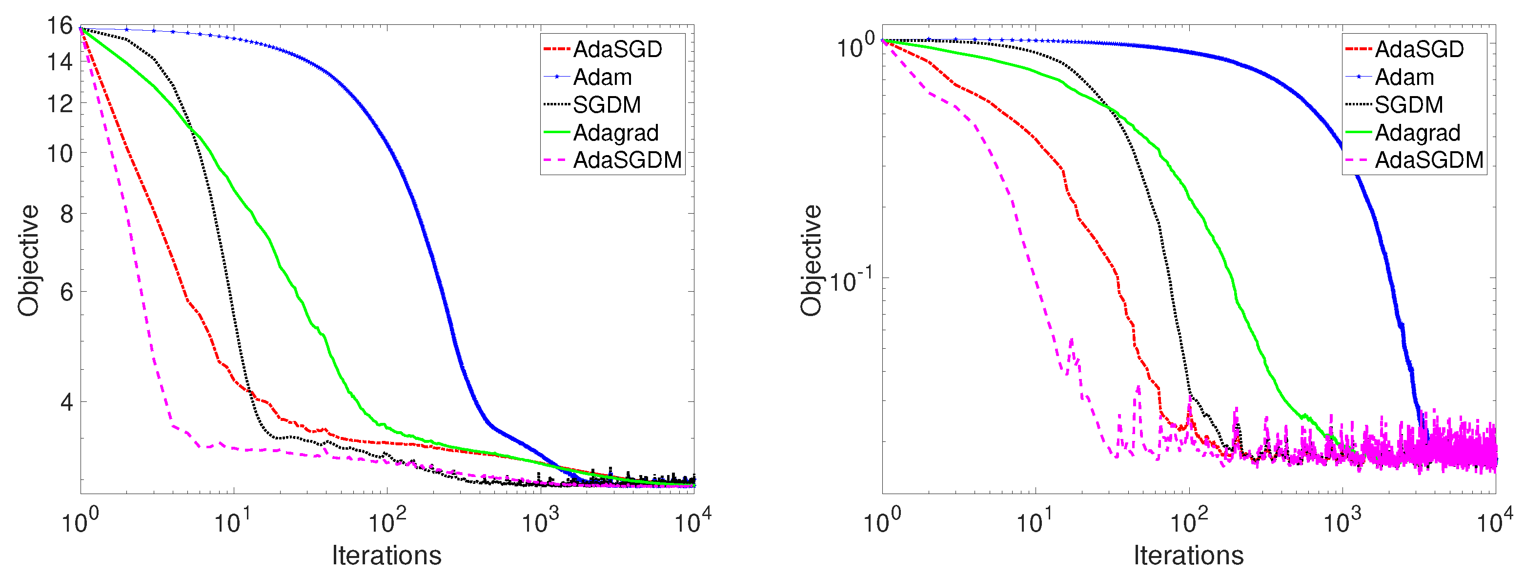
When $m=60$ and $n=10$, the convergence paths of the procedure for minimizing different convex functions in SGDM, Adam, Adagrad, and the proposed AdaSGD and AdaSGDM is demonstrated in Figure 1, where the left subfigure in Figure 1, corresponding to function $f_1\left(x\right)={\parallel Ax-b\parallel }^2+\lambda {\parallel x\parallel }_2^2$, takes 10.337139 s, and the right subfigure in Figure 1, corresponding to function $f_2\left(x\right)={\sum }_{i=1}^{m}log\left(1+e^{-b_i{A}_{i}x}\right)+\lambda {\parallel x\parallel }_2^2$, takes 4.947887 s. When $m=10,000$ and $n=200$. The results are shown in Figure 2, where the left and right subgraphs in Figure 2, corresponding to $f_1\left(x\right)$ and $f_2\left(x\right)$, take 2130.277402 s and 442.714215 s, respectively.

From the left and right figures in Figure 1 and Figure 2, it is not difficult to see that AdaSGD and AdaSGDM show better convergence than existing stochastic optimization methods when considering the convex optimization problems of different models. Observe that SGDM displays local acceleration close to the optimal point and attains convergence rate of $O(1/\sqrt{T})$, as shown in [36]. Adagrad shows a convergence rate of $O(1/\sqrt{T})$, as mentioned in [11]. Adam eventually attains a rate of convergence of $O(1/\sqrt{T})$, as shown in [10]. The proposed methods, AdaSGD and AdaSGDM, tend to converge faster than the SGDM, Adam, or Adagrad, showing a convergence of $1/T$, which is consistent with our theory results in this paper.

4.2. Non-Convex Functions

Consider the following non-convex support vector machine (SVM) problem with a sigmoid loss function, which has previously been considered in [5] (the data points are generated in the same way as in Section 4.1): ${min}_{x\in {\mathbb{R}}^n}{f}_3\left(x\right):={\sum }_{i=1}^m[1-tanh\left(b_i\langle x,a_i\rangle \right)]+\lambda {\parallel x\parallel }_2^2$, where $\lambda =0.1$ is a regularization parameter. In addition, consider the following non-convex optimization problem corresponding to the elastic regression network model [37]: ${min}_{x\in {\mathbb{R}}^n}{f}_4\left(x\right):=\parallel Ax-b\parallel -{\lambda }_1{\parallel x\parallel }_2^2+{\lambda }_2{\parallel x\parallel }_1$, where ${\lambda }_1=0.001$ and ${\lambda }_2=0.01$. Here, we use a mini-batch of size n to compute a stochastic gradient at each iteration. For minimizing the two non-convex functions $f_3\left(x\right)$ and $f_4\left(x\right)$, the gradient of $f_3\left(x\right)$ is obviously continuous. For $f_4\left(x\right)$ it is easy to know that the derivative of $f_4\left(x\right)$ at point $x=0$ does not exist; however, we can use the subgradient at this point. For example, one of the subgradients of $f_4\left(x\right)$ here is $\partial f_4\left(0\right)=0$. Although this gradient is discontinuous, it satisfies the Lipschitz condition, meaning that the conclusion in Theorem 3 holds. The convergence paths of the algorithms SGDM, Adam, Adagrad, AdaSGD, and AdaSGDM when ($m=60$, $n=10$) and ($m=10,000$, $n=200$) are shown in Figure 3 and Figure 4. The CPU times of the left and right subfigures corresponding to $f_3\left(x\right)$ and $f_4\left(x\right)$ in Figure 3 are 10.808409 s and 5.824761 s, respectively, and those of $f_3\left(x\right)$ and $f_4\left(x\right)$ in Figure 4 are 2369.346180 s and 455.041079 s, respectively.

From the figures in Figure 3 and Figure 4, it can be seen that AdaSGD and AdaSGDM maintain good convergence when considering non-convex optimization problems of different models. For different non-convex objective functions with Lipschitz continuous gradients, it can be observed that the gradient converges in expectation at the order of $O(1/\sqrt{T})$ of SGDM, as shown in [36]. As described in [10], the convergence analysis for Adam is not applicable to non-convex problems, and it is only through experience that Adam is likely to perform better than other methods. The Adagrad algorithm displays a convergence rate of $O(logT/\sqrt{T})$ under non-convex setting, as showed in [38]. For the proposed methods in this paper, AdaSGD and AdaSGDM, tend to converge faster than SGDM, Adam, and Adagrad under non-convex settings, showing a convergence of $1/T$, which is consistent with our theory result in this paper.

5. Conclusions and Future Work

In this paper, two shortcomings of the adaptive stochastic gradient descent method for stochastic optimization problems are studied. The first is the assumption of a convex setting, which is often harsh in many practical optimization problems of machine learning. The second is slow convergence, which is a result of using the adaptive step size of past stochastic gradients, and is generally up to $O(1/\sqrt{T})$. As a consequence, in this paper we first propose a new adaptive SGD in which the new step size is a function of the expectation of the past stochastic gradient and its second moment. In both convex and non-convex settings, the adaptive SGD with the new designed step size converges at the rate of $O(1/T)$. Second, the new adaptive SGD is extended to the case with momentum, and again achieves a convergence rate of $O(1/T)$, irrespective of convex or non-convex settings. To sum up, our results indicate that the designed adaptive step size is able to alleviate the problem of slow convergence caused by inherent variance to a certain extent. The proposed approach achieves accelerated convergence in convex setting, and works in non-convex settings as well. Experimental results show that the proposed adaptive stochastic gradient descent methods, both with and without momentum, have better convergence performance than existing methods. In the future, we hope to apply this method to large datasets or to actual data collection in order to better analyze its effectiveness.