Article

Front Propagation of Exponentially Truncated Fractional-Order Epidemics

1
Earth and Life Institute (ELI), Université Catholique de Louvain (UCLouvain), 1348 Louvain-la-Neuve, Belgium
2
Institute of Mechanics, Materials and Civil Engineering (IMMC), Université Catholique de Louvain (UCLouvain), 1348 Louvain-la-Neuve, Belgium
*
Author to whom correspondence should be addressed.
Fractal Fract. 2022, 6(2), 53; https://doi.org/10.3390/fractalfract6020053
Submission received: 27 November 2021 / Revised: 11 January 2022 / Accepted: 16 January 2022 / Published: 21 January 2022

Abstract

:
The existence of landscape constraints in the home range of living organisms that adopt Lévy-flight movement patterns, prevents them from making arbitrarily large displacements. Their random movements indeed occur in a finite space with an upper bound. In order to make realistic models, by introducing exponentially truncated Lévy flights, such an upper bound can thus be taken into account in the reaction-diffusion models. In this work, we have investigated the influence of the λ -truncated fractional-order diffusion operator on the spatial propagation of the epidemics caused by infectious diseases, where λ is the truncation parameter. Analytical and numerical simulations show that depending on the value of λ , different asymptotic behaviours of the travelling-wave solutions can be identified. For small values of λ ( λ 0 ), the tails of the infective waves can decay algebraically leading to an exponential growth of the epidemic speed. In that case, the truncation has no impact on the superdiffusive epidemics. By increasing the value of λ , the algebraic decaying tails can be tamed leading to either an upper bound on the epidemic speed representing the maximum speed value or the generation of the infective waves of a constant shape propagating at a minimum constant speed as observed in the classical models (second-order diffusion epidemic models). Our findings suggest that the truncated fractional-order diffusion equations have the potential to model the epidemics of animals performing Lévy flights, as the animal diseases can spread more smoothly than the exponential acceleration of the human disease epidemics.

1. Introduction

Infectious pathogens, such as viruses are the microorganisms that can cause infectious diseases following their presence and growth in humans and animals (hosts) [1]. One of the characteristics of infectious diseases is the ability of pathogens to be transmitted between individuals by either close contact between infected and non-infected (susceptible) individuals or a secondary host that carries the pathogens. Infectious diseases are thus also called communicable or transmissible diseases. Influenza, novel coronavirus (COVID-19), malaria, dengue fever, and West Nile virus are examples of infectious diseases. The propagation of infectious pathogens into non-infected regions leads to the spatial expansion of transmissible diseases and as a result, a large number of susceptible individuals can be infected so that an epidemic occurs. In some cases, a human epidemic can propagate over the entire globe, which is known as a pandemic. The 1918 Spanish influenza and COVID-19 are examples of classic and novel pandemics, respectively [2,3].
In epidemiology, mathematical models have been widely used to study the temporal and spatial dynamics of infectious diseases. Assuming the spatial homogeneity of the environment leads to the models that encompass the temporal dynamics of infectious diseases [4,5,6,7]. These models vary based on the characteristics of the particular disease, such as the transmission mechanism by either close contact or secondary hosts (see [8] for an extensive review of various mathematical models of animal and human infectious diseases). One of the purposes of such models is to derive the basic reproductive number that indicates the potential for the propagation of infectious diseases within a population. When its value is greater than unity, it shows that the infection is capable of invading the susceptible population, leading to the occurrence of an epidemic. Since this number is dependent on the model parameters, some strategies can be taken into account to control the propagation of the epidemics [9,10]. However, considering the random mobility of hosts and also the spatial heterogeneity of the environment lead to the reaction-diffusion models that describe the spatial dynamics of infectious diseases [11,12,13]. As an original model of this type, Källén et al. [14] studied the spatial spread of rabies among foxes. The main advantage of the reaction-diffusion epidemic models is to understand how fast an infectious disease can propagate. In that case, in order to control the spatial spread of the diseases, the parameters that govern the epidemic speed can be distinguished [15].
The type of host random mobility is a key factor that affects the epidemic speed and the patterns of the epidemic spread. Brownian motion and Lévy flight are two different patterns of random movements. Brownian motion is a normal dispersion process in which particles (walkers) make short movements such that the probability distribution function (pdf) of the displacement is obtained by the normal (Gaussian) distribution [16]. Considering Brownian motion pattern of susceptible and infective individuals leads to a second-order reaction-diffusion epidemic model. In that case, the epidemic waves propagate at a constant speed and the tails of the epidemic’s fronts decay exponentially. Such classical models have been applied to estimate the propagation speed of the plague in the 14th century and rabies in Europe [15,17]. However, Lévy-flight mobility pattern represents an anomalous diffusion process in which the walkers make occasionally large jumps between many short movements such that the pdf of the displacement is obtained by a power-law distribution with an asymptotic behaviour as l ( α + 1 ) , where l is the length of the displacement and 0 < α < 2 [18]. Different studies have shown that the random movement of many living organisms can be described by Lévy flights, including large marine predators [19,20], fruit flies [21], bumblebees [22], honeybees [23,24], albatrosses [25] and even humans [26]. Considering a population of the walkers performing a Lévy-flight mobility pattern leads to a fractional-order reaction-diffusion equation whose solution represents the walker densities [18,27]. From an applied point of view, fractional-order models have been used in a broad range of problems in ecology [28,29], biology [30], plasma turbulence [31,32], finance [33] and also recently numerous studies have been conducted on the subjects of bifurcation analysis, stability, and optimal control of fractional-order systems, such as predator-prey models [34,35], diffusive mussel-algae models [36], and neural networks [37,38,39]. As an application of space fractional-order diffusion equations in epidemiology, Hanert et al. [40] have shown that such equations can be applied to model the modern epidemics, such as avian influenza, and even SARS and also that the fractional-order diffusion operators make the epidemic waves travel at an exponential speed and the tails of the wave solutions decay algebraically as a power-law.
The existence of landscape and physiological constraints in the home range of living organisms following a pure Lévy-flight mobility pattern, can prevent arbitrarily large movements. To make realistic displacements, the tails of the power-law distribution must be truncated. In that case, the pure Lévy distribution is replaced by a truncated power-law distribution whose tail decays more quickly than it does in the pure Lévy case. Mantegna and Stanley [41] and Koponen [42] originally introduced truncated Lévy processes and after that Rosiński [43] proposed an exponentially truncated (tempered) Lévy process that yields a smoother decay than the abrupt cutoff. The pure power-law distributions result in diverging measurable quantities, such as variance and moments that cannot be observed in physically realizable systems. However, the truncated Lévy flight leads to the finite moments. The exponentially tempered Lévy distribution exhibits an asymptotic behaviour as ∼ e λ l l ( α + 1 ) , where l is the length of the displacement, 0 < α < 2 , and λ > 0 is the truncation parameter. When λ = 0 , it leads to a pure Lévy flight distribution. Considering a large number of random walkers performing a truncated Lévy flight leads to a truncated fractional-order diffusion equation whose solution represents the walker densities [44,45]. As an application of such equations, Vallaeys et al. [29] estimated isolation distances between genetically modified (GM) and non-GM crops by considering the fact that the honeybees mobility pattern can be well described by truncated Lévy flights. del Castillo Negrete [46] examined the influence of the truncation on the travelling-wave solutions of a truncated fractional-order Fisher–Kolmogorov equation. It would be of interest to investigate the results of such an equation in the epidemic models, as modern epidemics do not follow Brownian dynamics and can lead to accelerated waves of infectious diseases [47,48]. Hence, in this study, we apply the random mobility of infective individuals following truncated Lévy flights to an epidemic model and explore the epidemic speed based on the different values of the truncation parameter.
The remainder of the paper is organized as follows. In Section 2, we introduce the space fractional-order operators. In Section 3, we first review the classical and untruncated fractional-order epidemic models, then formulate a truncated fractional-order epidemic model and finally, discuss the epidemic speed of the new model. In Section 4, we explore our analytical results by numerically solving the model and conclusion is given in Section 5.

2. Preliminaries for Fractional-Order Operators

In this section, we shall give some definitions and notations that are required for this work. In the field of fractional models, the classical operators in time and/or space are replaced by the fractional derivative operators that are defined as follows.
For a given function f, the untruncated space fractional-order derivative operator of order α with a shorthand notation D x α or d α / d | x | α is defined as [44]:
D x α f ( x ) = l D x α f ( x ) + r x D α f ( x ) ,
where D x α and x D α are the positive (left) and negative (right) space-fractional Riemann–Liouville derivatives, respectively, defined as [49,50]:
D x α f ( x ) = 1 Γ ( n α ) n x n x f ( ξ ) ( x ξ ) α n + 1 d ξ ,
x D α f ( x ) = ( 1 ) n Γ ( n α ) n x n x f ( ξ ) ( ξ x ) α n + 1 d ξ ,
where Γ ( . ) denotes Euler’s gamma function and n = 1 + [ α ] such that [ α ] = max { m Z | m α } and Z is the set of integers. For instance, for 1 < α 2 , we get n = 2 , and the parameters l and r are the weighting factors defined as:
l = 1 β 2 cos ( α π / 2 ) , r = 1 + β 2 cos ( α π / 2 ) ,
where the parameter β [ 1 , 1 ] is a skewness parameter that shows a preferred direction of displacements that can be seen in heterogeneous systems. When β = 0 , the distribution is symmetric and space derivative represents a symmetric Riesz derivative.
Since the Riemann–Liouville derivatives are singular on the boundaries of a bounded domain [ 0 , L ] , where L > 0 , instead, Caputo derivatives can be used. The left and right Caputo derivatives of order α are defined as follow [49,50]:
0 c D x α f ( x ) = 1 Γ ( n α ) 0 x n f ( ξ ) / ξ n ( x ξ ) α n + 1 d ξ ,
x c D L α f ( x ) = ( 1 ) n Γ ( n α ) x L n f ( ξ ) / ξ n ( ξ x ) α n + 1 d ξ .
The λ truncated (tempered) fractional-order derivative operator of order α with a shorthand notation D x α , λ is defined as [44].
For 0 < α < 1 ,
D x α , λ f ( x ) = l e λ x D x α ( e λ x f ( x ) ) + r e λ x x D α ( e λ x f ( x ) ) + λ α cos ( α π / 2 ) f ( x ) ,
For 1 < α < 2 ,
D x α , λ f ( x ) = l e λ x D x α ( e λ x f ( x ) ) + r e λ x x D α ( e λ x f ( x ) ) + λ α cos ( α π / 2 ) f ( x ) + α β λ α 1 | cos ( α π / 2 ) | f x ,
where the operators D x α and x D α and the parameters l and r are defined by Equations (2)–(4), respectively, and λ 0 is a truncation parameter with SI units m 1 . Now, for 1 < α < 2 , we can define the left and right-sided truncated fractional-order operators D x α , λ and x D α , λ , for β = 1 and β = 1 , respectively, as follows:
D x α , λ f ( x ) = 1 cos ( α π / 2 ) e λ x D x α ( e λ x f ( x ) ) λ α f ( x ) α λ α 1 f x ,
x D α , λ f ( x ) = 1 cos ( α π / 2 ) e λ x x D α ( e λ x f ( x ) ) λ α f ( x ) + α λ α 1 f x ,

3. Spatial Propagation of an Epidemic

In this section, we investigate the effect of different random movements of individuals on the spatial spread and speed of an epidemic. To do so, we consider a simple version of the epidemic models. The model takes into account the densities of two populations at location x at time t, the susceptibles S ( x , t ) and the infectives I ( x , t ) . We assume that the susceptibles catch the disease from the infectives at a constant transmission-efficiency rate δ and that the infectives disappear either by recovery from the disease or disease-induced mortality, at a constant rate γ . We model the random movement of susceptibles and infectives by considering diffusion operators in the model equations. With these assumptions, the densities of susceptiples and infectives vary according to the following equations:
S t = δ S ( x , t ) I ( x , t ) + diffusion operator random motion ,
I t = δ S ( x , t ) I ( x , t ) γ I ( x , t ) + diffusion operator random motion ,
In what follows, we shall formulate “diffusion operator” by considering three patterns of random mobility of individuals, namely Brownian motion, pure (untruncated) Lévy flight and truncated Lévy flight, and then discuss the epidemic speed in each case.

3.1. Brownian Motion

Brownian motion is a normal dispersion process that the probability distribution function (pdf) for the displacements is a Gaussian (Normal) distribution. In that case, if we assume that the mobility of susceptible and infective individuals is described by Brownian motion, the diffusion operators in Equations (11) and (12) are the second-order diffusion denoted K 2 S ( x , t ) / x 2 and K 2 I ( x , t ) / x 2 , respectively, where K represents the diffusion coefficient and has units of m 2 s 1 . Therefore, we get
S t = δ S ( x , t ) I ( x , t ) + K 2 S ( x , t ) x 2 ,
I t = δ S ( x , t ) I ( x , t ) γ I ( x , t ) + K 2 I ( x , t ) x 2 ,
To obtain the epidemic speed, we consider a situation in which the wave of infectives propagates into the susceptible population whose density is uniformly set to be S ( x , 0 ) = S 0 throughout the entire domain. In that case, the constant epidemic speed at the leading edge, i.e., where S S 0 and I 0 is given by c = 2 K ( δ S 0 γ ) for K ( δ S 0 γ ) > 0 . For more details, refer to [15,17].

3.2. Pure (Untruncated) Lévy Flights

For pure Lévy flights, the power-law asymptotic behaviour of the pdf for the displacements leads to the space fractional-order diffusion operator D x α defined by Equation (1). If we assume that the susceptible and infective populations perform Lévy flights, the fractional-order epidemic model reads
S t = δ S ( x , t ) I ( x , t ) + K α D x α ,
I t = δ S ( x , t ) I ( x , t ) γ I ( x , t ) + K α D x α ,
where K α is the fractional-order diffusivity with units of m α s 1 . Hanert et al. [40] investigated the effect of the left-sided fractional diffusion operator on the left-and right-moving fronts. It was shown that the epidemic waves travel to the right side at an unbounded and exponential speed given by c ( t ) ( 1 λ ) e ( ( 1 λ ) / ( α + 1 ) ) t for large values of t and to the left side at a constant speed given by c = α ( ( 1 λ ) / ( α 1 ) ) ( α 1 ) / α , where λ = γ / δ S 0 . It should be noted that in the case of the symmetric fractional operator ( β = 0 ) , the infective waves propagating to the left and right sides have the same speed, i.e., both the left- and right-moving waves accelerate exponentially.

3.3. Truncated Lévy Flights

In this subsection, we investigate the effect of the truncated Lévy flights on the epidemic speed. To do so, we consider the left-sided truncated fractional-order diffusion operator D x α , λ defined by Equation (9). Since the movement of susceptible individuals does not change the front speed, for the sake of simplicity, we suppose that there is no diffusion term in the S equation. However, infectious individuals move into the susceptible population. The model equations then read as follows:
S ( x , t ) t = δ S ( x , t ) I ( x , t ) , I ( x , t ) t = δ S ( x , t ) I ( x , t ) γ I ( x , t )
+ D α e λ x D x α ( e λ x I ( x , t ) ) λ α I ( x , t ) ,
where D α = K α / | cos ( α π / 2 ) | . It should be noted that similar to the assumption used by del Castilo Negrete [46] for the truncated fractional-order Fisher–Kolmogorov equation, we do not consider the term I ( x , t ) / x in the I equation. In order to analyse the solutions of Equations (17) and (18), we first make them dimensionless by introducing the following variables:
S ¯ = S S 0 , I ¯ = I S 0 , x ¯ = x x c , t ¯ = t t c ,
where x c and t c are characteristic values of x and t, respectively. In what follows, we estimate these values. The next task is to insert the new dimensionless variables into Equations (17) and (18). That is, we replace S by S 0 S ¯ , I by S 0 I ¯ , t by t c t ¯ and x by x c x ¯ . The derivative with respect to t ¯ is derived through the chain rule as
I t = ( S 0 I ¯ ) t ¯ d t ¯ d t = S 0 I ¯ t ¯ 1 t c = S 0 t c I ¯ t ¯ , S t = S 0 t c S ¯ t ¯ ,
and the left fractional-order derivative with respect to x ¯ , D x ¯ α is also derived as follows:
D x α ( e λ x I ) = S 0 D x ¯ α ( e λ x c x ¯ I ¯ ) ( d x ¯ d x ) α = S 0 x c α D x ¯ α ( e λ x c x ¯ I ¯ ) .
Therefore, Equations (17) and (18) now become
S 0 t c S ¯ t ¯ = δ S 0 2 S ¯ I ¯ , S 0 t c I ¯ t ¯ = δ S 0 2 S ¯ I ¯ γ S 0 I ¯ + D α S 0 x c α e λ x c x ¯ D x ¯ α ( e λ x c x ¯ I ¯ ) D α λ α S 0 I ¯ ,
By choosing t c = 1 δ S 0 and x c = D α δ S 0 1 / α , we get the following model in a dimensionless form:
S ( x , t ) t = S ( x , t ) I ( x , t ) ,
I ( x , t ) t = S ( x , t ) I ( x , t ) θ I ( x , t ) + e μ x D x α ( e μ x I ( x , t ) ) ,
where we have dropped the overbar “−”, θ = γ + D α λ α δ S 0 , and μ = λ D α δ S 0 1 / α are dimensionless parameters.

3.3.1. Theoretical Analysis (Right-Propagating Front)

Here, we look for the speed of the infective waves propagating to the right side. Similar to the theoretical analysis of the model studied in [40], we replace S ( x , t ) by 1 s ( x , t ) , where s ( x , t ) is the deviation with respect to the initial density of the susceptible population. Since the epidemic speed can be obtained by the speed of the right-moving fronts in the leading edge region, i.e., where s 0 and I 0 , Equations (19) and (20) in that region can be expressed as
s ( x , t ) t = I ( x , t ) ,
I ( x , t ) t = ( 1 θ ) I ( x , t ) + e μ x D x α ( e μ x I ( x , t ) ) .
Here, we assume that 1 θ > 0 , which guarantees the existence of the right-moving fronts.
Now, we find the analytical solution of Equation (22), by defining the following localized initial condition:
I ( x , t = 0 ) = A if x < 0 A e ν x if x 0 ,
where A and ν are positive and non-zero constants. We next follow the same method as the one used by del Castilo Negrete [46] for the truncated fractional-order Fisher–Kolmogorov equation. First, we assume a solution of Equation (22) in the form of I ( x , t ) = e μ x + ( 1 θ ) t Φ ( x , t ) . By substituting this solution into (22) and initial condition (23), one gets the following fractional-order diffusion equation
Φ ( x , t ) t = D x α Φ ( x , t ) ,
with the initial condition
Φ 0 ( x ) = Φ ( x , t = 0 ) = A e μ x if x < 0 A e ( μ ν ) x if x 0 .
Equation (24) with initial condition (25) has the general solution of the form
Φ ( x , t ) = G ( x y , t ) Φ 0 ( y ) d y ,
where G ( x , t ) = t 1 / α p α ( x / t 1 / α ) is the Green function of Equation (24) and p α ( η ) = ( 1 / 2 π ) e ( i k ) α + i k η d k is a skewed Lévy distribution with exponent α . By substituting initial condition (25) into Equation (26), we get
Φ ( x , t ) = x t 1 / α A e ( μ ν ) ( x t 1 / α η ) p α ( η ) d η + x t 1 / α A e μ ( x t 1 / α η ) p α ( η ) d η = A e ( μ ν ) x x / τ e ( ν μ ) τ η p α ( η ) d η + A e μ x x / τ e μ τ η p α ( η ) d η ,
where τ = t 1 / α . Now, one can find the solution of Equation (22) in the following form
I ( x , t ) = A e ν x + ( 1 θ ) t I 1 + A e ( 1 θ ) t I 2 ,
where I 1 = x / τ e ( ν μ ) τ η p α ( η ) d η and I 2 = x / τ e μ τ η p α ( η ) d η .
The next task is to look for the asymptotic behaviour of the integrals I 1 and I 2 for x / τ with a fixed τ . We first consider the asymptotic behaviour of I 2 . By considering the fact that for η > 0 the Lévy distribution p α ( η ) exhibits fat tails as ∼ η ( α + 1 ) [46,51], and integration by parts, we get
I 2 x / τ e μ τ η η ( α + 1 ) d η = 1 μ τ e μ τ η η ( α + 1 ) η = x / τ η = α + 1 μ τ x / τ e μ τ η η ( α + 2 ) d η = τ α μ e μ x x α + 1 α + 1 μ τ x / τ e μ τ η η ( α + 2 ) d η τ α μ e μ x x α + 1 .
For the first integral I 1 , if we define a cutoff Ω with 1 Ω < x τ so that p α ( η ) η ( α + 1 ) , we can then write the integral I 1 as
I 1 Ω e ( ν μ ) τ η p α ( η ) d η + Ω x / τ e ( ν μ ) τ η η ( α + 1 ) d η .
Because of the exponential decay of p α ( η ) at minus infinity (for more details, refer to [46,51]), the first integral converges to a finite value C. By applying an integration by parts to the second integral of Equation (30), we get
Ω x / τ e ( ν μ ) τ η η ( α + 1 ) d η = 1 ( ν μ ) τ e ( ν μ ) τ η η ( α + 1 ) η = Ω η = x / τ + α + 1 ( ν μ ) τ Ω x / τ e ( ν μ ) τ η η ( α + 2 ) d η τ α ν μ e ( ν μ ) x x α + 1
Therefore,
I 1 C + τ α ν μ e ( ν μ ) x x α + 1 .
By substituting Equations (29) and (31) into Equation (28), we get
I ( x , t ) A C e ν x + ( 1 θ ) t + A 1 ν μ + 1 μ t x α + 1 e μ x + ( 1 θ ) t , ν μ , μ 0 .
In order to find the asymptotic behaviour of I ( x , t ) for large x, one can find the dominant term in Equation (32) by considering the relative values of ν and μ .
If μ < ν , the truncation decays slower than the initial condition. In that case, the second term of Equation (32) is the dominant term for large x, i.e.,
I ( x , t ) A 1 ν μ + 1 μ t x α + 1 e μ x + ( 1 θ ) t .
By considering the expansion of the exponential function e μ x , we get
I ( x , t ) A 1 ν μ + 1 μ t e ( 1 θ ) t 1 x α + 1 1 μ x + μ 2 2 x 2 .
For μ x 1 , the solution of I ( x , t ) thus decays algebraically as
I ( x , t ) t e ( 1 θ ) t x ( α + 1 ) ,
However, for μ x 1 , the algebraic decaying tail of the solution is tempered with the exponential factor e μ x as
I ( x , t ) t e μ x + ( 1 θ ) t x ( α + 1 ) .
If μ > ν , the truncation decays faster than the initial condition. In that case, the first term of Equation (32) is the dominant term for large x, i.e.,
I ( x , t ) e ν x + ( 1 θ ) t ,
which shows an exponentially decaying tail of the solution.
Until now, we have assumed that ν μ . To explore the case ν = μ , we cannot use Equation (32). Instead, we need to go back to Equation (30) and write the integral I 1 as
I 1 Ω p α ( η ) d η + Ω x / τ η ( α + 1 ) d η .
By defining the finite value C = Ω p α ( η ) d η and solving the second integral of Equation (38), we have
I 1 C τ α α 1 x α .
By substituting Equations (29) and (39) into (28), we obtain the solution I ( x , t ) as
I ( x , t ) A C e ν x + ( 1 θ ) t + A 1 μ x α + 1 1 α x α t e ν x + ( 1 θ ) t .
In this case, the first term of Equation (40) decays slower than the other term. Therefore, it is the dominant term for large x. We conclude that for the case ν = μ , the solution tail exhibits an exponentially decaying as
I ( x , t ) e ν x + ( 1 θ ) t
Obviously, the solution of Equation (21), the susceptibles equation, is obtained from the solution of the infectives equation. Thus, the asymptotic behaviour of the susceptible front is the same as the infective front.
The above results are based on the assumption μ 0 . However, in the absence of the truncation parameter, i.e., μ = 0 , we have to explore the asymptotic behaviour of the following integrals
I 1 = x / τ e ν τ η p α ( η ) d η , I 2 = x / τ p α ( η ) d η .
The analysis of the asymptotic behaviour of these integrals has been studied in [40] and it was shown that the solution I ( x , t ) has the same algebraically decaying tail as Equation (35).
In order to derive the epidemic speed, we first compute a Lagrangian trajectory x L ( t ) of infective fronts such that I ( x L ( t ) , t ) = I 0 , where I 0 0 . Given x L ( t ) , the epidemic speed is given by c ( t ) = d x L ( t ) / d t .
In the case of a power-law decaying tail, we find x L ( t ) from Equation (35) such that I ( x L ( t ) , t ) = t e ( 1 θ ) t x L ( t ) ( α + 1 ) = I 0 . After some calculation, x L ( t ) and c ( t ) can be computed as
x L ( t ) = I 0 1 / ( α + 1 ) t 1 / ( α + 1 ) e ( ( 1 θ ) / ( α + 1 ) ) t , c ( t ) ( 1 θ ) e ( ( 1 θ ) / ( α + 1 ) ) t .
For the truncated algebraically decaying tail, we use Equation (36) to find I ( x L ( t ) , t ) = t e μ x L ( t ) + ( 1 θ ) t x L ( t ) ( α + 1 ) = I 0 . Thus, x L ( t ) satisfies the following equation
ln t + ( 1 θ ) t μ x L ( t ) ( α + 1 ) ln x L ( t ) = ln I 0 ,
and c ( t ) can be expressed as
c ( t ) = ( 1 θ ) + 1 t μ + α + 1 x L ( t ) .
When t , the velocity of the fronts converges towards a constant value representing the maximum value of the epidemic speed given by c m a x = ( 1 θ ) / μ .
Finally, in the case of exponentially decaying tail, we can use Equation (37) to find I ( x L ( t ) , t ) = e ν x L ( t ) + ( 1 θ ) t = I 0 . Thus, x L ( t ) = ( ln I 0 + ( 1 θ ) t ) / ν and the front moves at a constant velocity c ( t ) = c ¯ = ( 1 θ ) / ν .

3.3.2. Theoretical Analysis (Left-Propagating Front)

For exploring the impact of the left-sided truncated operator defined by Equation (9) on the left-moving fronts, we consider a travelling-wave solution of a constant shape as follows:
I ( x , t ) = I ( z ) , s ( x , t ) = s ( z ) , z = x + c t ,
where c represents the speed of the epidemic waves moving to the left side. Substituting this solution into Equations (21) and (22), one can find the following system:
c s z = I ,
c I z = ( 1 θ ) I + e μ z D z α ( e μ z I ) .
Now we define a solution of the following form
I ( z ) = I ^ e k z , s ( z ) = s ^ e k z ,
where k is a parameter depending on the value of c. Considering the fact that D z α e k z = k α e k z and substituting the solutions (48) into Equations (46) and (47), we get the following system:
c k 1 0 c k ( k + μ ) α ( 1 θ ) s ^ I ^ = 0 0 .
If c k ( c k ( k + μ ) α ( 1 θ ) ) = 0 , we can find a non-trivial solution. In that case, we get the following relation representing the value of the epidemic speed as a function of the parameter k:
c ( k ) = 1 θ k + ( k + μ ) α k .
In order to obtain the minimum epidemic speed, one can minimize Equation (50) with respect to k. For 0 < α < 2 and μ 0 , we cannot analytically calculate the minimum speed c m i n . In the next section, we thus find it numerically. However, for 0 < α < 2 and μ = 0 , as it is discussed in [40], c m i n = α ( 1 θ ) / ( α 1 ) ( α 1 ) / α and the corresponding rate of the exponential decay is equal to k m i n = ( 1 θ ) / ( α 1 ) 1 / α . For α = 2 , the minimum speed of the classical model is given by c m i n = 2 1 θ .

4. Numerical Examples

In order to illustrate the analytical results obtained for the asymptotic behaviour of the infective waves, we numerically solve the model equations on a finite domain [ 0 , L ] , where L > 0 . Here, we have used the same method as the one performed by Vallaeys et al. [29] for solving a symmetric truncated fractional-order diffusion equation. To study more numerical methods for solving the space fractional-order diffusion equations, refer to [52,53,54]. We discretize Equations (19) and (20) by finite-element (FE) method based on a Galerkin formulation. To illustrate this method more precisely, we discretize the following simple diffusion equation:
I ( x , t ) t = e λ x 0 D x α ( e λ x I ( x , t ) ) λ α I ( x , t ) .
In this method, the exact solution (unknown variable) I ( x , t ) is expressed as a sum of the unknown coefficients e j ( t ) and basis functions ϕ j ( x ) as follows:
I ( x , t ) I ˜ ( x , t ) = j = 1 N e j ( t ) ϕ j ( x ) .
By introducing a partition of the domain [ 0 , L ] into N 1 subintervals [ x j , x j + 1 ] with a constant length h, i.e., x 1 = 0 , x N = L , and x j + 1 x j = h for j = 1 , , N 1 , we can consider the piecewise linear basis functions ϕ j ( x ) for j = 1 , 2 , , N as follows:
ϕ 1 ( x ) = x 2 x x 2 x 1 : x 1 x x 2 , 0 : x [ x 1 , x 2 ] .
for j = 2 , , N 1 ,
ϕ j ( x ) = x x j 1 x j x j 1 : x j 1 x x j , x j + 1 x x j + 1 x j : x j x x j + 1 , 0 : x [ x j 1 , x j + 1 ] .
and for j = N ,
ϕ N ( x ) = x x N 1 x N x N 1 : x N 1 x x N , 0 : x [ x N 1 , x N ] .
We also discretize the exponentially truncated unknown solution, i.e., e λ x I ( x , t ) as follows
e λ x I ( x , t ) I ˜ l ( x , t ) = j = 1 N e j l ( t ) ϕ j ( x ) .
where e j l ( t ) is the unknown coefficient corresponding to the left truncated solution.
By using a Galerkin formulation, we replace I ˜ ( x , t ) and I ˜ l ( x , t ) in Equation (51) and then by orthogonalizing the discrete equation with respect to all ϕ j , we get the following equation:
0 L ϕ i ϕ j d x d e j d t ( t ) = 0 L ϕ i e λ x 0 D x α ϕ j d x e j l ( t ) λ α 0 L ϕ i ϕ j d x e j ( t ) ,
for i , j = 1 , , N .
By introducing the matrices M : = 0 L ϕ i ϕ j d x and D : = 0 L ϕ i e λ x 0 D x α ϕ j d x , we get the following semi-discrete equation in a matrix form
M d e d t ( t ) = D e l ( t ) λ α M e ( t ) ,
where e ( t ) = e 1 ( t ) e N ( t ) T and e l ( t ) = e 1 l ( t ) e N l ( t ) T are the vector of unknown coefficients at time t. It should be noted that by considering the same method in [55], the diffusion matrix D can be expressed as: D = 0 L e λ x ( d ϕ i d x λ ϕ i ) 0 D x α 1 ϕ j d x . Here we use the left Caputo derivative of order α 1 of ϕ j defined by Equation (5) as Caputo derivatives are easier to handle and also for many applications could prevent mass-balance errors on bounded domains, while such errors can be made by Riemann–Liouville derivatives (for more details, see [56]).
In order to solve Equation (54), the vector e l ( t ) needs to be computed in terms of the vector e ( t ) . To do so, we use Galerkin formulation for Equations (52) and (53) as follows:
0 L ϕ i e λ x I ˜ d x = 0 L ϕ i I ˜ l d x 0 L ϕ i e λ x ϕ j d x e j ( t ) = 0 L ϕ i ϕ j d x e j l ( t ) .
By defining the matrix W : = 0 L ϕ i e λ x ϕ j d x , we get e l ( t ) = M 1 W e ( t ) . we can thus express Equation (54) as follows
M d e d t ( t ) = D M 1 W λ α M e ( t ) ,
Finally, in order to discretize Equation (55), we use a third-order Adams–Bashforth method.
In order to solve the model Equations (19) and (20), we use the following initial conditions:
S ( x , t = 0 ) = S 0 ( x ) = 1 h S 1 ± tanh ( x x 0 w s L ) ,
I ( x , t = 0 ) = I 0 ( x ) = h I e ν ( x x 0 ) : x x 0 , h I e ν ( x x 0 ) : x x 0 ,
where h S = 0.37 , w S = 0.003 , h I = 0.14 , and ν = 0.001 . we consider the “+” sign and x 0 = 9 L / 10 for the left-moving front and the “−” sign and x 0 = L / 30 for the right-moving front. The dimensionless length of the domain is set to L = 10 5 and L = 3 × 10 5 for the left- and right-moving fronts, respectively. For all simulations, θ = 0.5 , and the value of the fractional order α is set to 1.2 . According to the analytical results, we can consider three different asymptotic behaviours for the right-moving fronts, i.e., y 1 = x ( α + 1 ) (power-law decay), y 2 = e μ x x ( α + 1 ) (truncated power-law decay), and y 3 = e μ x (exponential decay). In what follows, we shall show how different values of the truncation parameter μ lead to these different asymptotic behaviours.
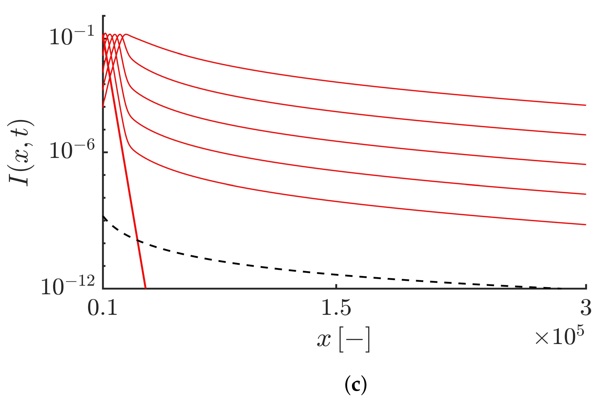
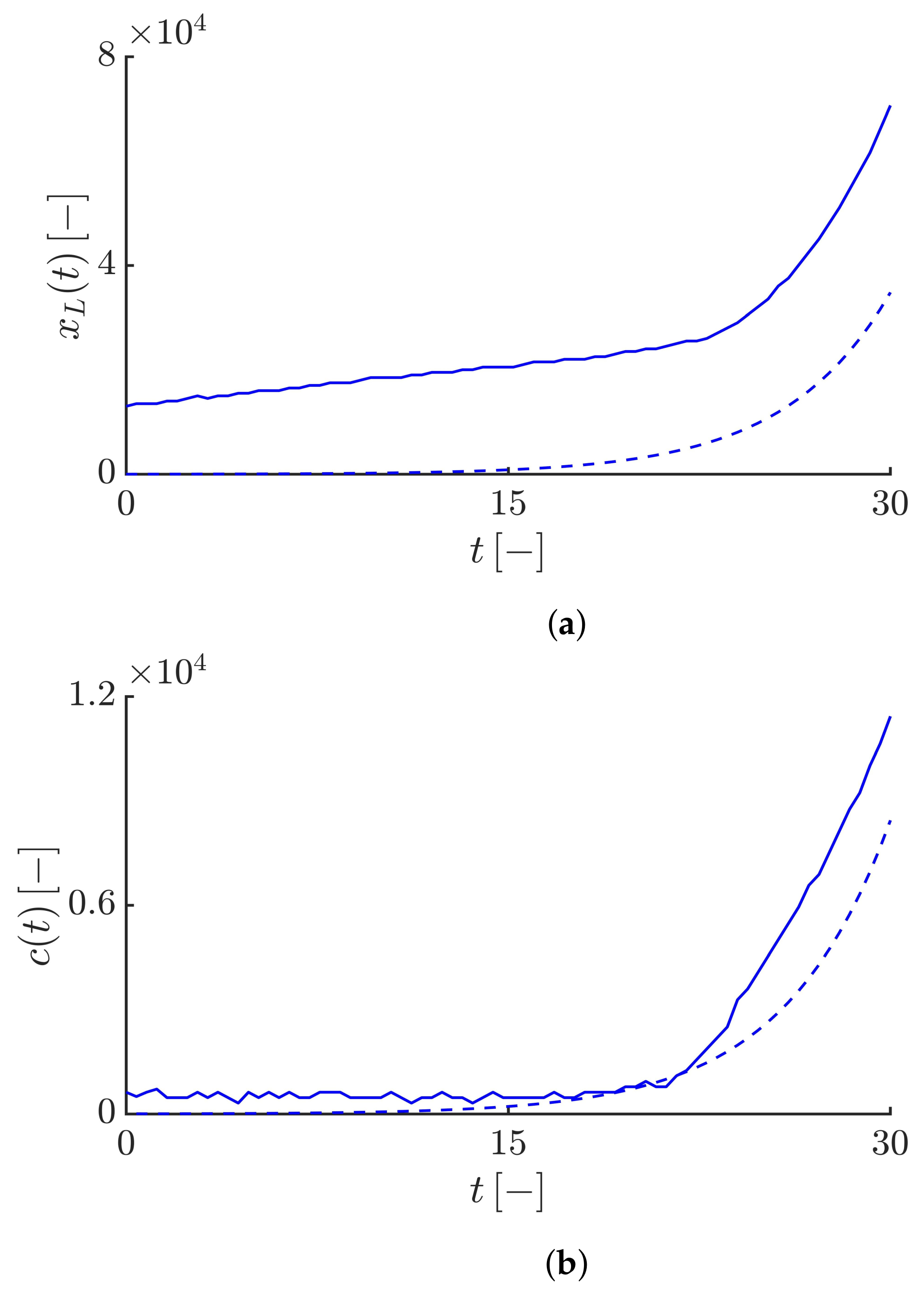
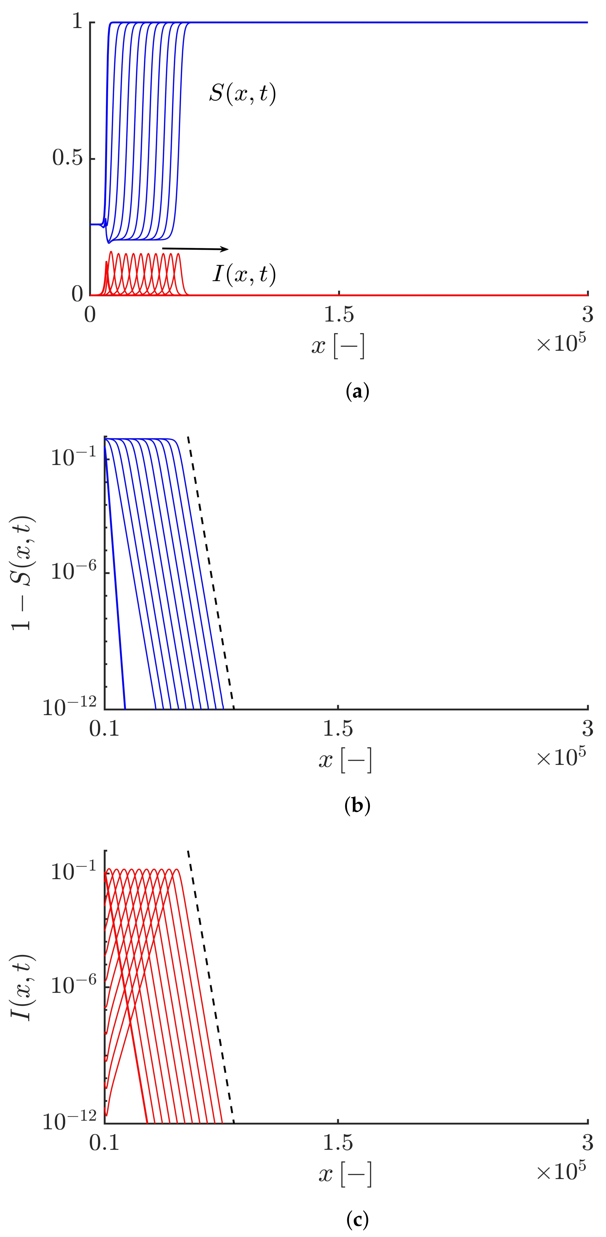
The algebraic decaying tail of the right-moving fronts are shown in Figure 1. Here, we take μ = 5 × 10 6 < ν . Figure 1a shows the densities of both the susceptibles and infectives at different times. Figure 1b,c show that the right-moving fronts for both the susceptibles and infectives exhibit a power-law decaying tail as y 1 = x ( α + 1 ) . The Lagrangian trajectory x L ( t ) and the epidemic speed c ( t ) corresponding to this case are shown in Figure 2a,b, respectively. Figure 2a shows the time evolution of the Lagrangian trajectory x L ( t ) such that I ( x L ( t ) , t ) = I 0 , where I 0 = 0.01 . Figure 2b shows the time evolution of the numerical estimation of the instantaneous speed of the points with density I 0 = 0.01 . Both Figure 2a,b also show that the results obtained numerically agree well with the asymptotic expansions obtained by Equation (43). It should be noted that the truncation parameter here has no influence on the rapid propagation of the epidemic and the fronts move at an exponential speed similar to the fractional-order epidemic model based on pure Lévy flights [40].
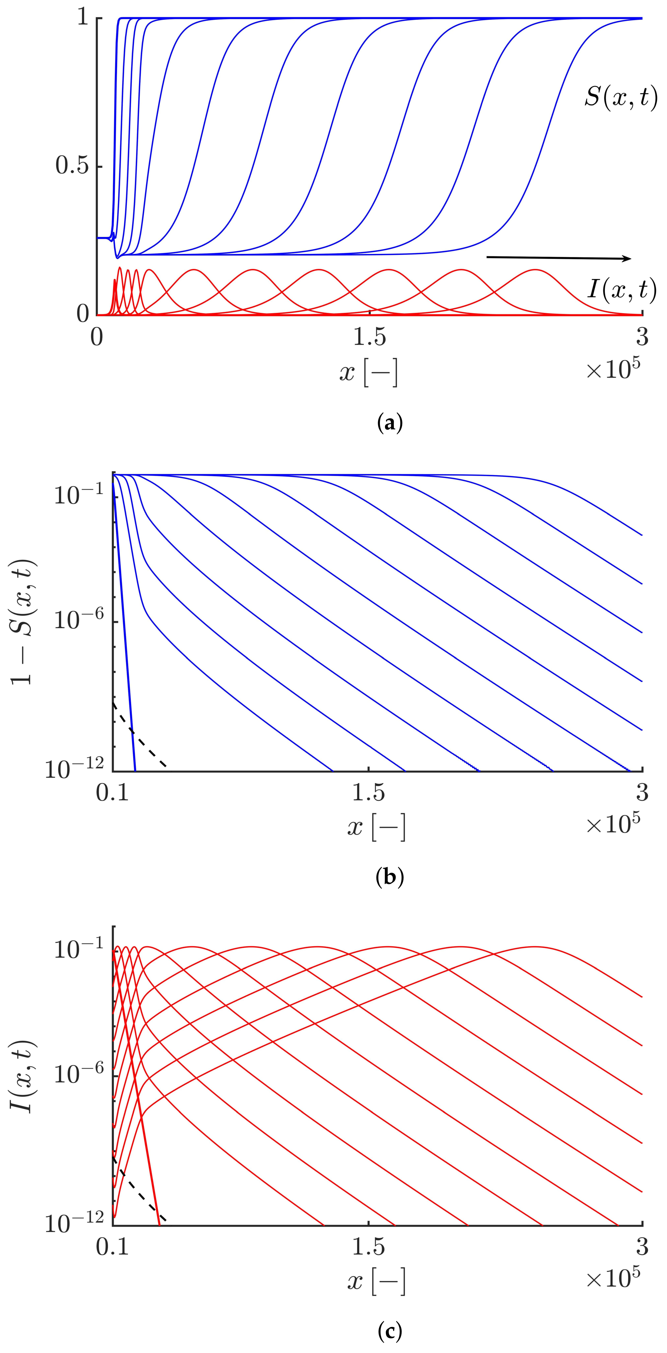
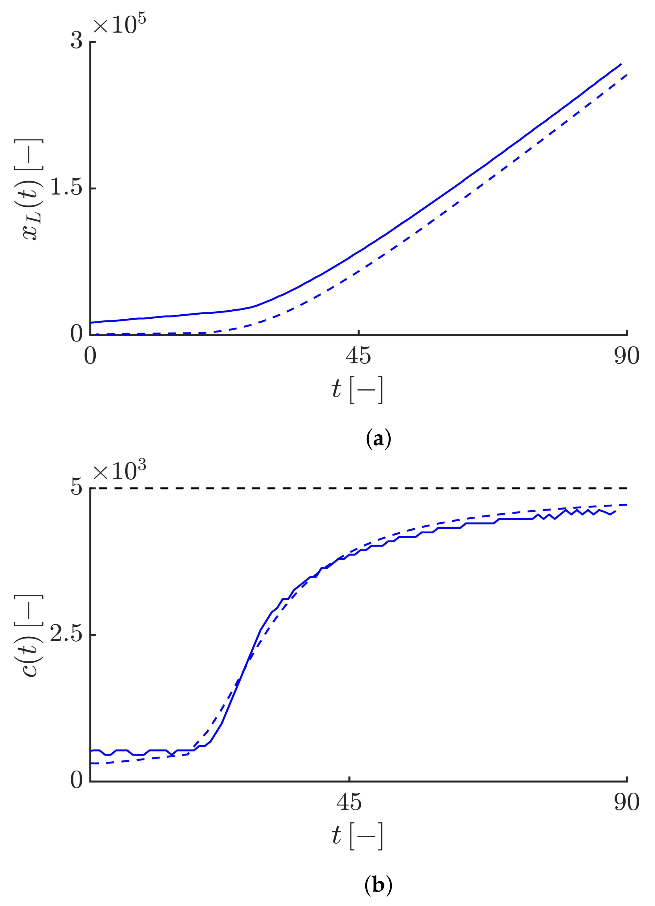
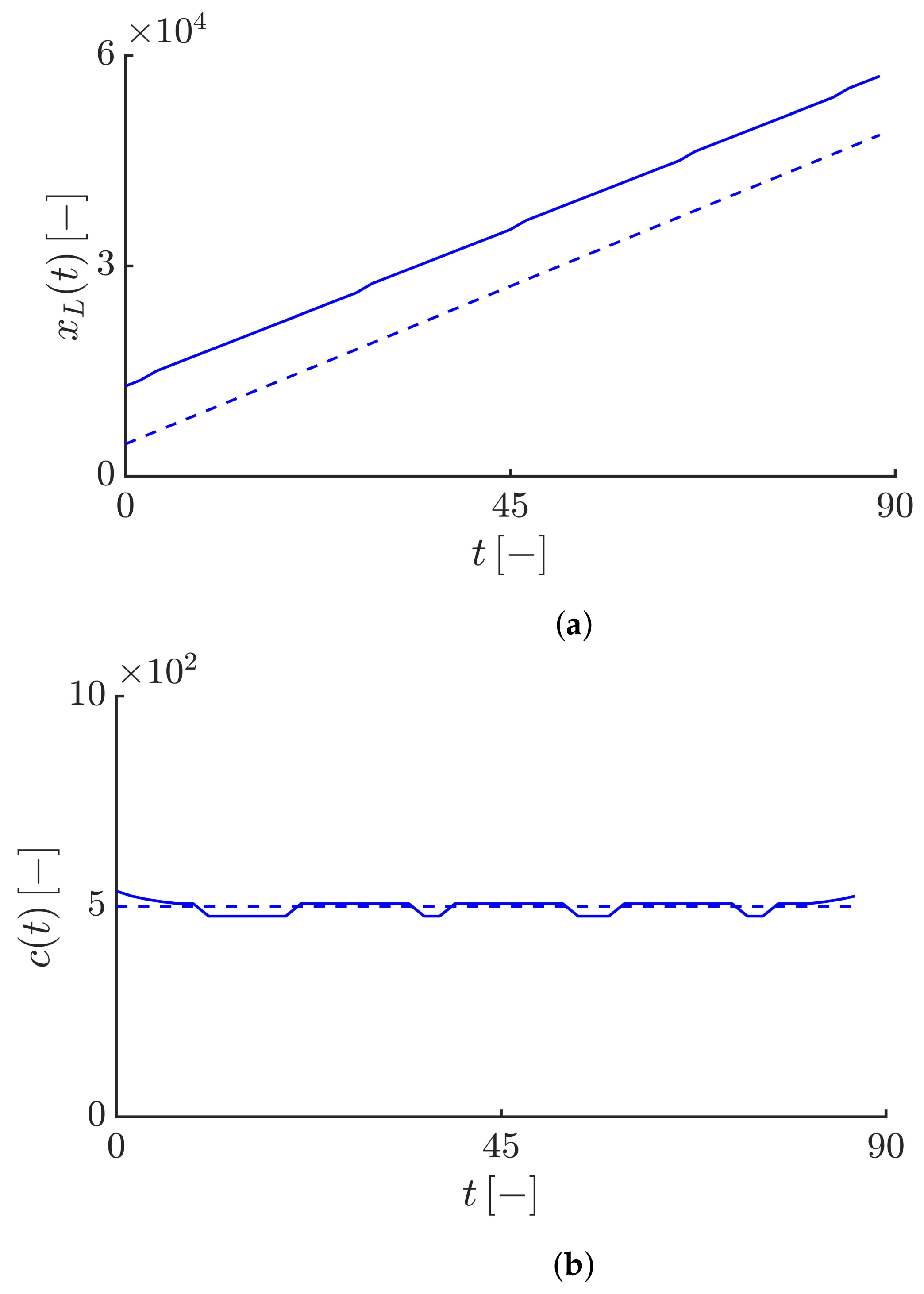
By increasing the value of the truncation parameter μ , the algebraically decaying tail of the solutions can be tamed. If we take μ = 10 4 < ν , both the susceptible and infective fronts propagate so that their tails exhibit a tempered algebraic decaying, i.e., 1 S and I y 2 = e μ x x ( α + 1 ) (see Figure 3). Figure 4 shows that the Lagrangian trajectory x L ( t ) and the velocity c ( t ) obtained by numerically solving Equations (19) and (20) are in good agreement with the results obtained analytically by Equations (44) and (45). As expected, the infective fronts initially propagate at the minimum average speed c m i n = 5 × 10 2 and then the front speed gradually increases so that after some time, it converges towards the maximum front speed value c m a x = 5 × 10 3 .
Figure 5 shows the dynamics of the right-moving susceptible and infective fronts for μ = 10 3 . As expected, for μ ν , the tails of the solutions for the susceptible and infective fronts exhibit an exponential decay, i.e, 1 S and I y 3 = e ν x (see Figure 5b,c). Figure 6 shows that the Lagrangian trajectory x L ( t ) and the velocity c ( t ) obtained by numerically solving the model equations are in good agreement with the analytical results. In this case, similar to the classical epidemic models, the infective fronts propagate at a constant speed c = 5 × 10 2 . It should be noted that since in the first case ( μ = 5 × 10 6 ) , the epidemic fronts propagate over the entire domain during a shorter time compared to the other cases ( μ = 10 4 and μ = 10 3 ) , for the first case, we consider the simulation duration equals 30. However, for the others, it is equal to 90.
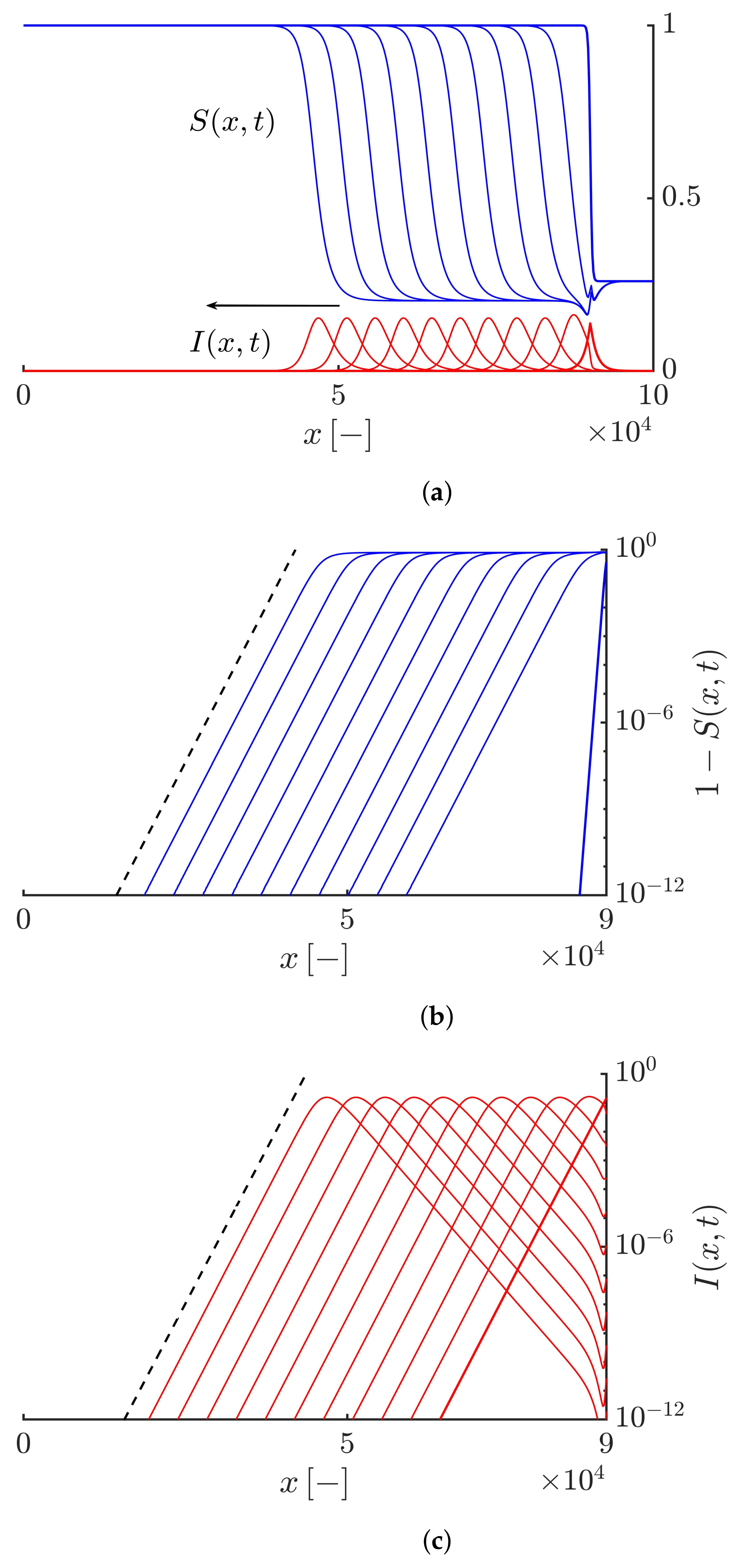
Figure 7 shows the time evolution of the susceptible and infective waves propagating to the left side. Figure 7a shows the densities of the susceptibles and infectives at different times. Figure 7b,c show that the tails of the solutions decay exponentially as ∼ y = e ν x . Here, the simulation duration is equal to 90. In this case, for all values of the truncation parameter, the fronts move at a constant velocity that is equal to c = 5 × 10 2 .
It should be noted that when we consider both the left-and right-sided truncated fractional-order diffusion operators by choosing the strict values of the skewness parameter β , i.e., 1 < β < 1 , ( β = 0 leads to a symmetric operator), both the left- and right-sided derivatives affect the epidemic speed and the asymptotic behaviour of the front’s tail. In that case, both the left- and right-moving front tails exhibit the same asymptotic behaviour based on the values of the truncation parameter. For instance, if the truncation parameter μ is set to 10 4 , the tails of both the left- and right-moving fronts decay as ∼ e μ x x ( α + 1 ) .
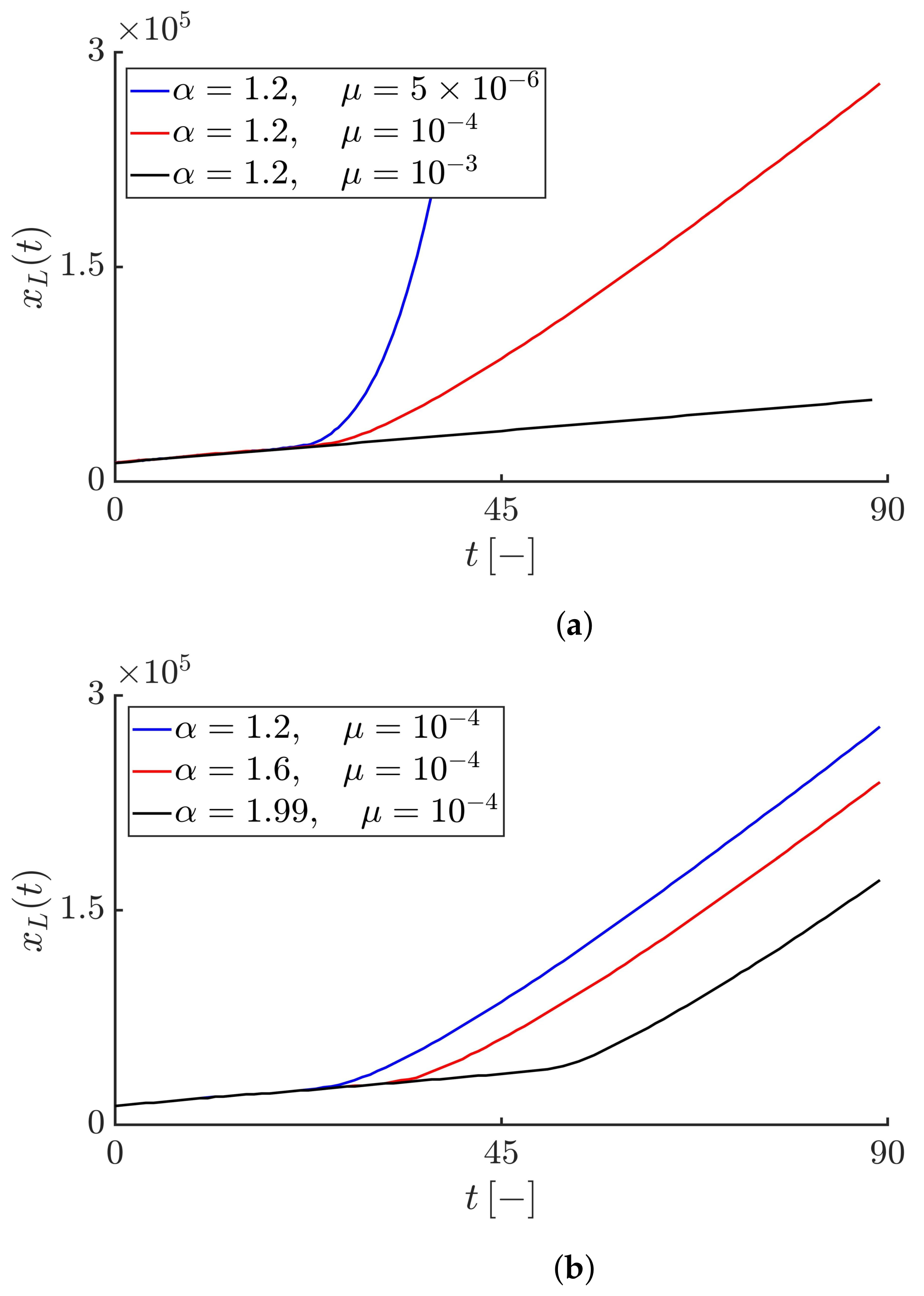
Figure 8a shows the time evolution of the Lagrangian trajectory x L ( t ) for the constant value of the fractional-order derivative α = 1.2 and different values of the truncation parameter μ . As we see, in all cases, the values of x L ( t ) initially increase linearly at a constant speed on average equals 5 × 10 2 and then, for μ = 5 × 10 6 , x L ( t ) increases exponentially leading to an exponential and unbounded velocity of the infective fronts (see Figure 2b), but for μ = 10 4 , x L ( t ) increases gradually leading to the convergence of the epidemic speed to the maximum velocity value c m a x 5 × 10 3 (see Figure 4b), and finally for μ = 10 3 , x L ( t ) increases linearly leading to the constant speed c = 5 × 10 2 (see Figure 6b).
Figure 8b shows the time evolution of the Lagrangian trajectory x L ( t ) for different values of the fractional-order derivative α and a constant value of the truncation parameter μ = 10 4 . Since, the value of μ is constant, in all cases the Lagrangian velocity converges towards a plateau showing the maximum average speed, but the time to reach that plateau is not the same for different values of α . As we see, the smaller the value of α , i.e., the closer it is to 1, the faster the Lagrangian trajectory accelerates leading to the faster convergence of the front speed towards the maximum speed compared to values of α that are closer to 2.

5. Conclusions

In this work, we have investigated the spatial propagation of the epidemics caused by infectious diseases. We have considered a simple version of the epidemic models consisting of susceptible and infective populations. The diffusion process resulting from the random mobility of the infective individuals is taken into account in our model. Based on the previous studies, in the case of the Brownian motion, the infective waves propagate into the susceptible population at a constant speed and the tails of the travelling-wave solutions exhibit an exponential decay, while in the case of pure (untruncated) Lévy flights, the left-sided fractional derivative leads to an exponential and unbounded speed of the infective waves moving to the right side, but generates a constant speed at the left side. In that case, right-moving fronts have an algebraic tail. However, left-moving fronts exhibit an exponential tail.
As a new study, we have applied the truncated Lévy flight to the proposed model. Similar to the results obtained for the λ -truncated fractional-order Fisher–Kolmogorov Equation [46], for the right-moving fronts, we have shown that the epidemic speed is dependent on the level of the truncation parameter. In this case, we have considered a left-sided truncated fractional-order diffusion operator. For small values of λ ( λ 0 ), the tails of the infective waves can decay algebraically leading to an exponential growth of the epidemics. In that case, the truncation has no impact on the superdiffusive epidemics. By increasing the value of λ , the algebraic decaying tails can be tamed leading to either an upper bound on the epidemic speed representing the maximum speed or the generation of the infective waves of a constant shape propagating at a minimum constant speed similar to the classical models (second-order diffusion epidemic models). For the left-moving fronts, our numerical results show that for different values of the truncation parameter, the truncated left-sided fractional derivative generates the waves of a constant shape moving at a constant speed. Obviously, considering the strict values of the skewness parameter β , i.e., 1 < β < 1 , leads to the effect of both the left-and right-sided truncated fractional-order diffusion operators on the epidemic speed. In that case, based on the value of the truncation parameter, the tails of both the left- and right-moving fronts have the same asymptotic behaviour.
From an applied perspective, the untruncated power laws (pure Lévy flights) have some drawbacks. As discussed in [57], in nature, due to the finite space, landscape and physiological limitations, the occurrence of arbitrarily large displacements by the individuals following a pure Lévy flight is not realistic. In that case, one individual cannot make displacements beyond an upper bound. By introducing truncated power-laws, such an upper bound can thus be taken into account in the fractional-order diffusion models. As mentioned by Hanert et al. [40], since modern epidemics caused by human infectious diseases can propagate over the entire globe very quickly, the untruncated fractional-order diffusion epidemic models can better represent such epidemics. However, concerning the infectious diseases of animals doing a Lévy flight, the propagation of the epidemics is more smooth, our findings thus suggest that truncated fractional-order diffusion models are more appropriate for modelling the animal diseases.
The space fractional-order epidemic models could be further improved by considering the non-Markovian diffusion processes in which the pdf for waiting times between displacements have a power-law asymptotic behaviour as ∼ τ ( γ + 1 ) , where 0 < γ < 1 . In that case, the time derivative of order one is replaced by a time fractional derivative of order γ [18]. As an example of such diffusion processes, Brockmann et al. [26] observed that the dispersion of bank notes has memory effects. In order to numerically solve time-space fractional diffusion equations, Hanert [52] has proposed an efficient and flexible scheme.

Author Contributions

Conceptualization, A.F. and E.H.; Methodology, A.F.; Supervision, E.H.; Writing—original draft, A.F.; Writing—review and editing, A.F. and E.H. All authors have read and agreed to the published version of the manuscript.

Funding

UCLouvain International Relations Office.

Data Availability Statement

Available upon request to the author.

Conflicts of Interest

The authors declare no conflict of interest.

References

  1. Cleaveland, S.; Laurenson, M.K.; Taylor, L.H. Diseases of humans and their domestic mammals: Pathogen characteristics, host range and the risk of emergence. Philos. Trans. R. Soc. London. Ser. B Biol. Sci. 2001, 356, 991–999. [Google Scholar] [CrossRef] [PubMed]
  2. Nelson, K.E.; Williams, C.M. Infectious Disease Epidemiology: Theory and Practice; Jones & Bartlett Publishers: Burlington, MA, USA, 2014. [Google Scholar]
  3. Ciotti, M.; Ciccozzi, M.; Terrinoni, A.; Jiang, W.C.; Wang, C.B.; Bernardini, S. The COVID-19 pandemic. Crit. Rev. Clin. Lab. Sci. 2020, 57, 365–388. [Google Scholar] [CrossRef] [PubMed]
  4. Brauer, F. Modeling influenza: Pandemics and seasonal epidemics. In Mathematical Epidemiology; Springer: Berlin/Heidelberg, Germany, 2008; pp. 321–347. [Google Scholar]
  5. Cruz-Pacheco, G.; Esteva, L.; Montaño-Hirose, J.A.; Vargas, C. Modelling the dynamics of West Nile virus. Bull. Math. Biol. 2005, 67, 1157–1172. [Google Scholar] [CrossRef] [PubMed]
  6. Esteva, L.; Vargas, C. Analysis of a dengue disease transmission model. Math. Biosci. 1998, 150, 131–151. [Google Scholar] [CrossRef]
  7. Chen, Y.C.; Lu, P.E.; Chang, C.S.; Liu, T.H. A time-dependent SIR model for COVID-19 with undetectable infected persons. IEEE Trans. Netw. Sci. Eng. 2020, 7, 3279–3294. [Google Scholar] [CrossRef]
  8. Keeling, M.J.; Rohani, P. Modeling Infectious Diseases in Humans and Animals; Princeton University Press: Princeton, NJ, USA, 2011. [Google Scholar]
  9. Van den Driessche, P.; Watmough, J. Further notes on the basic reproduction number. In Mathematical Epidemiology; Springer: Berlin/Heidelberg, Germany, 2008; pp. 159–178. [Google Scholar]
  10. Bowman, C.; Gumel, A.; Van den Driessche, P.; Wu, J.; Zhu, H. A mathematical model for assessing control strategies against West Nile virus. Bull. Math. Biol. 2005, 67, 1107–1133. [Google Scholar] [CrossRef] [PubMed]
  11. Wu, J. Spatial structure: Partial differential equations models. In Mathematical Epidemiology; Springer: Berlin/Heidelberg, Germany, 2008; pp. 191–203. [Google Scholar]
  12. Maidana, N.A.; Yang, H.M. Spatial spreading of West Nile Virus described by traveling waves. J. Theor. Biol. 2009, 258, 403–417. [Google Scholar] [CrossRef]
  13. Maidana, N.A.; Yang, H.M. Describing the geographic spread of dengue disease by traveling waves. Math. Biosci. 2008, 215, 64–77. [Google Scholar] [CrossRef]
  14. Källén, A.; Arcuri, P.; Murray, J. A simple model for the spatial spread and control of rabies. J. Theor. Biol. 1985, 116, 377–393. [Google Scholar] [CrossRef]
  15. Murray, J.D. Mathematical Biology II: Spatial Models and Biomedical Applications; Springer: New York, NY, USA, 2001; Volume 3. [Google Scholar]
  16. Okubo, A.; Levin, S.A. Diffusion and Ecological Problems: Modern Perspectives; Springer: New York, NY, USA, 2001; Volume 14. [Google Scholar]
  17. Shigesada, N.; Kawasaki, K. Biological Invasions: Theory and Practice; Oxford University Press: Oxford, UK, 1997. [Google Scholar]
  18. Metzler, R.; Klafter, J. The random walk’s guide to anomalous diffusion: A fractional dynamics approach. Phys. Rep. 2000, 339, 1–77. [Google Scholar] [CrossRef]
  19. Humphries, N.E.; Queiroz, N.; Dyer, J.R.; Pade, N.G.; Musyl, M.K.; Schaefer, K.M.; Fuller, D.W.; Brunnschweiler, J.M.; Doyle, T.K.; Houghton, J.D.; et al. Environmental context explains Lévy and Brownian movement patterns of marine predators. Nature 2010, 465, 1066–1069. [Google Scholar] [CrossRef] [PubMed] [Green Version]
  20. Sims, D.W.; Southall, E.J.; Humphries, N.E.; Hays, G.C.; Bradshaw, C.J.; Pitchford, J.W.; James, A.; Ahmed, M.Z.; Brierley, A.S.; Hindell, M.A.; et al. Scaling laws of marine predator search behaviour. Nature 2008, 451, 1098–1102. [Google Scholar] [CrossRef] [PubMed]
  21. Reynolds, A.M.; Frye, M.A. Free-flight odor tracking in Drosophila is consistent with an optimal intermittent scale-free search. PLoS ONE 2007, 2, e354. [Google Scholar] [CrossRef] [PubMed] [Green Version]
  22. Lihoreau, M.; Ings, T.C.; Chittka, L.; Reynolds, A.M. Signatures of a globally optimal searching strategy in the three-dimensional foraging flights of bumblebees. Sci. Rep. 2016, 6, 30401. [Google Scholar] [CrossRef] [Green Version]
  23. Reynolds, A.M.; Smith, A.D.; Menzel, R.; Greggers, U.; Reynolds, D.R.; Riley, J.R. Displaced honey bees perform optimal scale-free search flights. Ecology 2007, 88, 1955–1961. [Google Scholar] [CrossRef] [PubMed]
  24. Reynolds, A.M.; Smith, A.D.; Reynolds, D.R.; Carreck, N.L.; Osborne, J.L. Honeybees perform optimal scale-free searching flights when attempting to locate a food source. J. Exp. Biol. 2007, 210, 3763–3770. [Google Scholar] [CrossRef] [PubMed] [Green Version]
  25. Humphries, N.E.; Weimerskirch, H.; Sims, D.W. A new approach for objective identification of turns and steps in organism movement data relevant to random walk modelling. Methods Ecol. Evol. 2013, 4, 930–938. [Google Scholar] [CrossRef]
  26. Brockmann, D.; Hufnagel, L.; Geisel, T. The scaling laws of human travel. Nature 2006, 439, 462–465. [Google Scholar] [CrossRef]
  27. Chaves, A. A fractional diffusion equation to describe Lévy flights. Phys. Lett. A 1998, 239, 13–16. [Google Scholar] [CrossRef]
  28. Hanert, E. Front dynamics in a two-species competition model driven by Lévy flights. J. Theor. Biol. 2012, 300, 134–142. [Google Scholar] [CrossRef]
  29. Vallaeys, V.; Tyson, R.C.; Lane, W.D.; Deleersnijder, E.; Hanert, E. A Lévy-flight diffusion model to predict transgenic pollen dispersal. J. R. Soc. Interface 2017, 14, 20160889. [Google Scholar] [CrossRef] [PubMed]
  30. Raghib, M.; Levin, S.A.; Kevrekidis, I.G. Multiscale analysis of collective motion and decision-making in swarms: An advection–diffusion equation with memory approach. J. Theor. Biol. 2010, 264, 893–913. [Google Scholar] [CrossRef] [PubMed] [Green Version]
  31. del Castillo-Negrete, D.; Carreras, B.; Lynch, V. Fractional diffusion in plasma turbulence. Phys. Plasmas 2004, 11, 3854–3864. [Google Scholar] [CrossRef]
  32. del Castillo-Negrete, D.; Carreras, B.; Lynch, V. Nondiffusive transport in plasma turbulence: A fractional diffusion approach. Phys. Rev. Lett. 2005, 94, 065003. [Google Scholar] [CrossRef] [PubMed] [Green Version]
  33. Cartea, A.; del Castillo-Negrete, D. Fractional diffusion models of option prices in markets with jumps. Phys. A Stat. Mech. Its Appl. 2007, 374, 749–763. [Google Scholar] [CrossRef] [Green Version]
  34. Yuan, J.; Zhao, L.; Huang, C.; Xiao, M. Stability and bifurcation analysis of a fractional predator–prey model involving two nonidentical delays. Math. Comput. Simul. 2021, 181, 562–580. [Google Scholar] [CrossRef]
  35. Huang, C.; Liu, H.; Chen, X.; Zhang, M.; Ding, L.; Cao, J.; Alsaedi, A. Dynamic optimal control of enhancing feedback treatment for a delayed fractional order predator–prey model. Phys. A Stat. Mech. Its Appl. 2020, 554, 124136. [Google Scholar] [CrossRef]
  36. Djilali, S.; Ghanbari, B.; Bentout, S.; Mezouaghi, A. Turing-Hopf bifurcation in a diffusive mussel-algae model with time-fractional-order derivative. Chaos Solitons Fractals 2020, 138, 109954. [Google Scholar] [CrossRef]
  37. Xu, C.; Liao, M.; Li, P.; Guo, Y.; Liu, Z. Bifurcation properties for fractional order delayed BAM neural networks. Cogn. Comput. 2021, 13, 322–356. [Google Scholar] [CrossRef]
  38. Huang, C.; Nie, X.; Zhao, X.; Song, Q.; Tu, Z.; Xiao, M.; Cao, J. Novel bifurcation results for a delayed fractional-order quaternion-valued neural network. Neural Netw. 2019, 117, 67–93. [Google Scholar] [CrossRef] [PubMed]
  39. Xu, C.; Zhang, W.; Aouiti, C.; Liu, Z.; Liao, M.; Li, P. Further investigation on bifurcation and their control of fractional-order bidirectional associative memory neural networks involving four neurons and multiple delays. Math. Methods Appl. Sci. 2021, 1–24. [Google Scholar] [CrossRef]
  40. Hanert, E.; Schumacher, E.; Deleersnijder, E. Front dynamics in fractional-order epidemic models. J. Theor. Biol. 2011, 279, 9–16. [Google Scholar] [CrossRef] [Green Version]
  41. Mantegna, R.N.; Stanley, H.E. Stochastic process with ultraslow convergence to a Gaussian: The truncated Lévy flight. Phys. Rev. Lett. 1994, 73, 2946. [Google Scholar] [CrossRef]
  42. Koponen, I. Analytic approach to the problem of convergence of truncated Lévy flights towards the Gaussian stochastic process. Phys. Rev. E 1995, 52, 1197. [Google Scholar] [CrossRef]
  43. Rosiński, J. Tempering stable processes. Stoch. Process. Their Appl. 2007, 117, 677–707. [Google Scholar] [CrossRef] [Green Version]
  44. Cartea, Á.; del Castillo-Negrete, D. Fluid limit of the continuous-time random walk with general Lévy jump distribution functions. Phys. Rev. E 2007, 76, 041105. [Google Scholar] [CrossRef] [PubMed] [Green Version]
  45. Baeumer, B.; Meerschaert, M.M. Tempered stable Lévy motion and transient super-diffusion. J. Comput. Appl. Math. 2010, 233, 2438–2448. [Google Scholar] [CrossRef] [Green Version]
  46. del Castillo-Negrete, D. Truncation effects in superdiffusive front propagation with Lévy flights. Phys. Rev. E 2009, 79, 031120. [Google Scholar] [CrossRef] [PubMed] [Green Version]
  47. Small, M.; Walker, D.M.; Tse, C.K. Scale-free distribution of avian influenza outbreaks. Phys. Rev. Lett. 2007, 99, 188702. [Google Scholar] [CrossRef] [Green Version]
  48. Mundt, C.C.; Sackett, K.E.; Wallace, L.D.; Cowger, C.; Dudley, J.P. Long-distance dispersal and accelerating waves of disease: Empirical relationships. Am. Nat. 2009, 173, 456–466. [Google Scholar] [CrossRef] [PubMed]
  49. Samko, S.G.; Kilbas, A.A.; Marichev, O.I. Fractional Integrals and Derivatives: Theory and Applications; Gordon and Breach: New York, NY, USA, 1993. [Google Scholar]
  50. Podlubny, I. Fractional Differential Equations: An Introduction to Fractional Derivatives, Fractional Differential Equations, to Methods of Their Solution and Some of Their Applications; Elsevier: Amsterdam, The Netherlands, 1998. [Google Scholar]
  51. Mainardi, F.; Luchko, Y.; Pagnini, G. The fundamental solution of the space-time fractional diffusion equation. arXiv 2007, arXiv:cond-mat/0702419. [Google Scholar]
  52. Hanert, E. On the numerical solution of space-time fractional diffusion models. Comput. Fluids 2011, 46, 33–39. [Google Scholar] [CrossRef]
  53. Piret, C.; Hanert, E. A radial basis functions method for fractional diffusion equations. J. Comput. Phys. 2013, 238, 71–81. [Google Scholar] [CrossRef]
  54. Hanert, E.; Piret, C. A Chebyshev pseudospectral method to solve the space-time tempered fractional diffusion equation. SIAM J. Sci. Comput. 2014, 36, A1797–A1812. [Google Scholar] [CrossRef]
  55. Hanert, E. A comparison of three Eulerian numerical methods for fractional-order transport models. Environ. Fluid Mech. 2010, 10, 7–20. [Google Scholar] [CrossRef]
  56. Zhang, X.; Lv, M.; Crawford, J.W.; Young, I.M. The impact of boundary on the fractional advection–dispersion equation for solute transport in soil: Defining the fractional dispersive flux with the Caputo derivatives. Adv. Water Resour. 2007, 30, 1205–1217. [Google Scholar] [CrossRef]
  57. Viswanathan, G.M.; Raposo, E.; Da Luz, M. Lévy flights and superdiffusion in the context of biological encounters and random searches. Phys. Life Rev. 2008, 5, 133–150. [Google Scholar] [CrossRef]
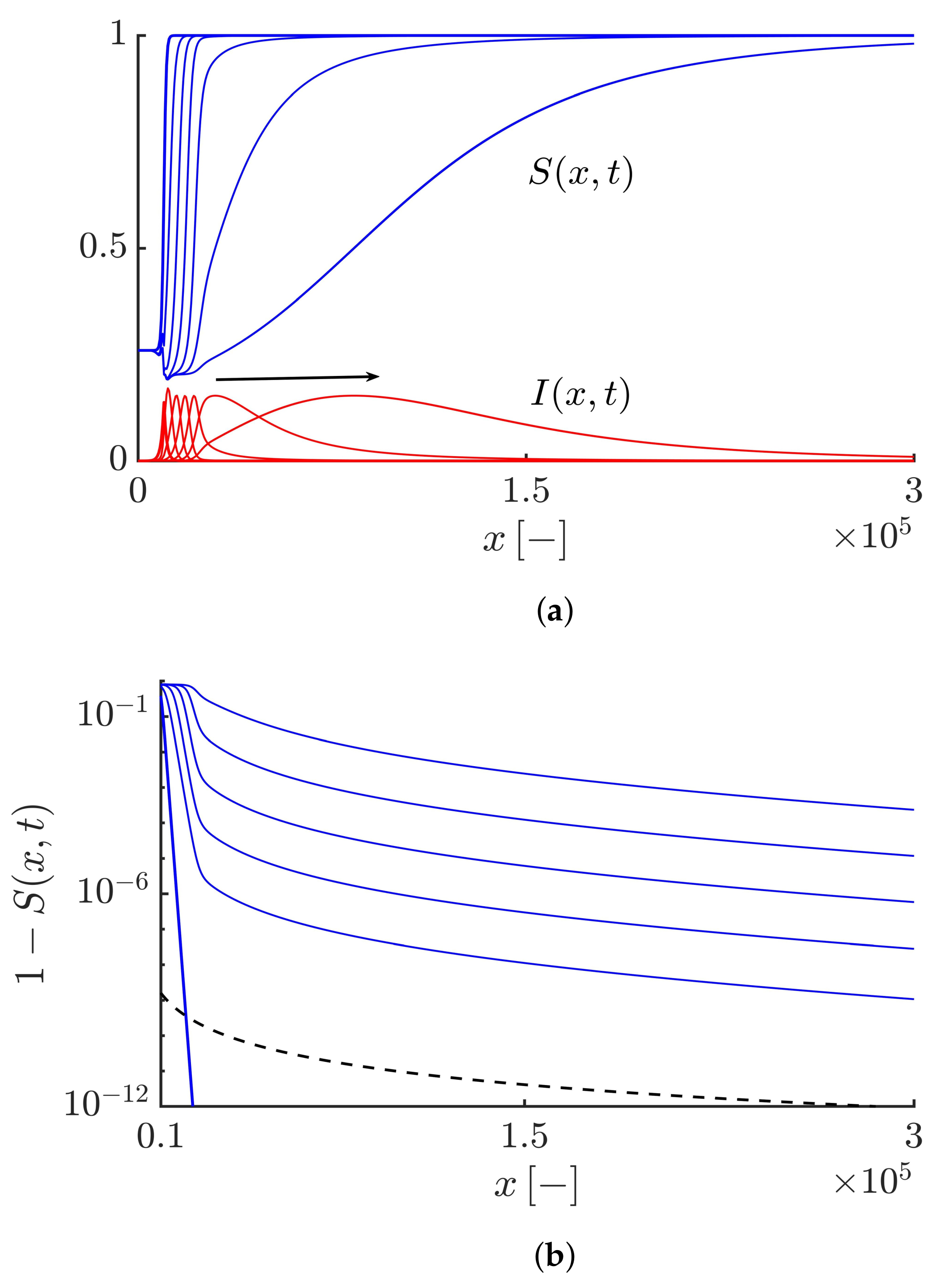
Figure 1. (a) Profiles of the susceptible and infective waves moving to the right side at different times obtained by solving Equations (19) and (20) with α = 1.2 and μ = 5 × 10 6 < ν . The arrow shows the direction of the front propagation. (b,c) Highlighting an algebraic decaying tail for the susceptible and infective waves, i.e., 1 S and I y 1 = x ( α + 1 ) shown by the black dashed curves. The duration of the simulation and the time interval between curves equal 30 and 6, respectively.
Fractalfract 06 00053 g001aFractalfract 06 00053 g001b
Figure 2. (a) Time evolution of the Lagrangian trajectory x L ( t ) at the leading edge of the infective waves such that I ( x L ( t ) , t ) = I 0 , where I 0 = 0.01 . The value of μ is equal to 5 × 10 6 . The dashed curve corresponds to the asymptotic expansion of the Lagrangian trajectory, i.e., x L ( t ) t 1 / ( α + 1 ) e ( ( 1 θ ) / ( α + 1 ) ) t . (b) Time evolution of the instantaneous velocity of the right-propagating infective waves obtained by c ( t ) = d x L ( t ) / d t . The dashed curve corresponds to the asymptotic expansion of the Lagrangian velocity, i.e., c ( t ) ( 1 θ ) e ( ( 1 θ ) / ( α + 1 ) ) t , highlighting the exponential speed of the epidemic and also the agreement of the numerical result with the analytical velocity.
Fractalfract 06 00053 g002
Figure 3. (a) Profiles of the susceptible and infective waves moving to the right side at different times obtained by solving Equations (19) and (20) with α = 1.2 and μ = 10 4 < ν . The arrow shows the direction of the front propagation. (b,c) Highlighting an exponentially tempered algebraic decaying tail for the susceptible and infective waves, i.e., 1 S and I y 2 = e μ x x ( α + 1 ) shown by the black dashed curves. The duration of the simulation and the time interval between curves equal 90 and 9, respectively.
Fractalfract 06 00053 g003
Figure 4. (a) Time evolution of the Lagrangian trajectory x L ( t ) at the leading edge of the infective waves such that I ( x L ( t ) , t ) = I 0 , where I 0 = 0.01 . The value of μ is equal to 10 4 . The dashed curve corresponds to the analytical Lagrangian trajectory satisfies in the equation ln t + ( 1 θ ) t μ x L ( t ) ( α + 1 ) ln x L ( t ) = ln I 0 . (b) Time evolution of the instantaneous velocity of the right-propagating infective waves obtained by c ( t ) = d x L ( t ) / d t . The dashed curve corresponds to the analytical Lagrangian velocity obtained by c ( t ) = ( ( 1 θ ) + 1 / t ) / ( μ + ( α + 1 ) / x L ( t ) ) , highlighting the agreement of the numerical result with the analytical velocity and also the convergence of the epidemic speed towards the maximum epidemic speed value c m a x 5 × 10 3 (see the black dashed line).
Fractalfract 06 00053 g004
Figure 5. (a) Profiles of the susceptible and infective waves moving to the right side at different times obtained by solving Equations (19) and (20) with α = 1.2 and μ = 10 3 = ν . The arrow shows the direction of the front propagation. (b,c) Highlighting an exponential decaying tail for the susceptible and infective waves, i.e., 1 S and I y 3 = e ν x shown by the back dashed curves. The duration of the simulation and the time interval between curves equal 90 and 9, respectively.
Fractalfract 06 00053 g005
Figure 6. (a) Time evolution of the Lagrangian trajectory x L ( t ) at the leading edge of the infective waves such that I ( x L ( t ) , t ) = I 0 , where I 0 = 0.01 . The value of μ is equal to 10 3 . The dashed curve corresponds to the asymptotic expansion of the Lagrangian trajectory, i.e., x L ( t ) = ( ln I 0 + ( 1 θ ) t ) / ν . (b) Time evolution of the instantaneous velocity of the right-propagating infective waves obtained by c ( t ) = d x L ( t ) / d t . The dashed curve corresponds to the constant Lagrangian velocity, i.e., c ( t ) = c ¯ = ( 1 θ ) / ν , highlighting the agreement of the numerical result with the analytical velocity.
Fractalfract 06 00053 g006
Figure 7. (a) Profiles of the susceptible and infective waves moving to the left side at different times obtained by solving Equations (19) and (20) with α = 1.2 and different values of the truncation parameter μ = 5 × 10 6 , 10 4 and 10 3 . The arrow shows the direction of the front propagation. (b,c) Highlighting an exponential decaying tail for the susceptible and infective waves, i.e., 1 S and I y = e ν x shown by the black dashed curves. The duration of the simulation and the time interval between curves equal 90 and 9, respectively.
Fractalfract 06 00053 g007
Figure 8. (a) Time evolution of the Lagrangian trajectory for fractional-order derivative α = 1.2 and different values of the truncation parameter μ . The blue, red and black curves correspond to μ = 5 × 10 6 , μ = 10 4 , and μ = 10 3 , respectively. (b) Time evolution of the Lagrangian trajectory for different values of the fractional-order derivative α and the truncation parameter μ = 10 4 . The blue, red and black curves correspond to α = 1.2 , α = 1.6 , and α = 1.99 , respectively.
Fractalfract 06 00053 g008
Publisher’s Note: MDPI stays neutral with regard to jurisdictional claims in published maps and institutional affiliations.