Article

A New Numerical Scheme for Time Fractional Diffusive SEAIR Model with Non-Linear Incidence Rate: An Application to Computational Biology

by
Yasir Nawaz
1,2,
Muhammad Shoaib Arif
1,3,* and
Wasfi Shatanawi
3,4,5
1
Department of Mathematics, Air University, PAF Complex E-9, Islamabad 44000, Pakistan
2
Department of Sciences and Humanities, National University of Computer and Emerging Sciences, Islamabad 44000, Pakistan
3
Department of Mathematics and Sciences, College of Humanities and Sciences, Prince Sultan University, Riyadh 11586, Saudi Arabia
4
Department of Medical Research, China Medical University, Taichung 40402, Taiwan
5
Department of Mathematics, Faculty of Science, The Hashemite University, P.O. Box 330127, Zarqa 13133, Jordan
*
Author to whom correspondence should be addressed.
Fractal Fract. 2022, 6(2), 78; https://doi.org/10.3390/fractalfract6020078
Submission received: 30 December 2021 / Revised: 26 January 2022 / Accepted: 27 January 2022 / Published: 31 January 2022
(This article belongs to the Special Issue Fractional Dynamical Systems: Applications and Theoretical Results)

Abstract

:
In this paper, we propose a modified fractional diffusive SEAIR epidemic model with a nonlinear incidence rate. A constructed model of fractional partial differential equations (PDEs) is more general than the corresponding model of fractional ordinary differential equations (ODEs). The Caputo fractional derivative is considered. Linear stability analysis of the disease-free equilibrium state of the epidemic model (ODEs) is presented by employing Routh–Hurwitz stability criteria. In order to solve this model, a fractional numerical scheme is proposed. The proposed scheme can be used to find conditions for obtaining positive solutions for diffusive epidemic models. The stability of the scheme is given, and convergence conditions are found for the system of the linearized diffusive fractional epidemic model. In addition to this, the deficiencies of accuracy and consistency in the nonstandard finite difference method are also underlined by comparing the results with the standard fractional scheme and the MATLAB built-in solver pdepe. The proposed scheme shows an advantage over the fractional nonstandard finite difference method in terms of accuracy. In addition, numerical results are supplied to evaluate the proposed scheme’s performance.

1. Introduction

Nowadays, the world faces the contagious outcomes of a fatal pathogen called coronavirus [1], which belongs to the family of SARS-CoV-2. Viruses of this family can transfer their pathogenicity to humans and animals. In humans, they affect the respiratory tract, injure the digestive lining, and cause severe gastroenteritis. Lung disorders may vary from mild cold to acute degenerative respiratory syndrome that ultimately becomes a cause of death. Precautionary and preventive measures have been taken at the government level to contain the virus to save the economy and health system from collapse. This situation of uncertainty between life and death has opened a new gospel in the field of quantitative mathematical modeling. Civil society and philanthropists are turning towards numerical modeling to gain insight to control the spread of the virus and predict possible measures to reduce cases. Many researchers have imparted fruitful numerical contributions on epidemic situations in the past decades. Bernoulli’s work among those researchers has a notable significance in epidemiology, as his studies were pioneering against smallpox disease. In 1927, Kermack and McKendrick developed an epidemic modeling technique that has recently provided the basis for COVID-19 modeling. However, epidemiologists are still struggling to better understand the COVID-19 virus and effective measures for its containment [2].
In the COVID-19 epidemiological model, scientists prefer to add factors such as the exposed population. The addition of more compartments will increase the model’s suitability and refine the description with the assumption of transfer of infection from one class to another [3,4,5]. The best possible coronavirus solution is vaccination. Alternatively, the confinement of susceptible individuals will limit their proportion. In this regard, the simulation model has its value. Such models provide crucial tools and gather efforts to slow the pathogen’s spread to save lives.
Due to its diverse and distinctive qualities, fractional calculus has grown substantially. The non-integer order derivative is solved using fractional calculus techniques discussed further below. Fractional calculus is the generalization of conventional calculus and has around a 300-year-old history. Fractional calculus is an effective tool for describing many systems. There are various disciplines where fractional calculus has been used, including electrochemistry and water transport at the ground level, elasticity, geology, distribution, heat conduction, and electromagnetism and elasticity. Recently, it has been recognized that fractional operators are more appropriate tools for differentiation than local operators, particularly for physical, real-world problems. It has long been recognized that fractional derivatives are more relevant than ordinary derivatives when modeling various real-world physic-mathematical phenomena. Fractional operators are defined by convolutions of fractional operators’ kernels with their local derivatives.
Unlike integer-order models, different biological models offer subsequent memory effects. These models are based on inheritance introduced through the ABC operator, a substantial property of the biological process. In the modeling of biological processes, fractional operators have gained increasing interest. A detailed review of [6] revealed a proposed SEIHDR model comprising an ABC operator to study the dynamics of COVID-19. In [7,8], new fractional derivatives have been introduced for theoretical and application aspects of the heat transfer model and application to the Baggs and Freedman model.
In December 2019, the first case of COVID-19 was reported in Wuhan, a province of China. Since then, more cases have been reported in China and worldwide, making this pandemic a universal warning. High case numbers and exponential death rates urged the World Health Organization to declare COVID-19 a global health emergency. The recent focus of many scholars is to produce a model of COVID-19 based on a system of differential equations and devise some suitable means to restrict the spread of the virus. A careful investigation of [9] found that the efficacy of treatment response would influence whether an endemic scenario is to emerge inside a community or not. Furthermore, the author of [9] applied the SEIR model to the COVID-19 scenario, derived the basic reproduction number, and proved the local and global stabilities of the disease-free and endemic states.
The SEIR model utilized in [9] is the addition of the SERIUS model investigated in [10,11]. In this model, S stands for the susceptible group, E stands for exposed individuals to a particular pathogen, I refer to an infectious class, and R stands for the recovered group. U is an undetected class obtained by collapsing the undetected and recovered class only then when they appear as COVID-19-negative twice in PCR tests. In 2017, the Centers for Disease Control declared that the SERIUS model was formulated on the principle that there is no re-infection after recovery. Today, there is no evidence that individuals who recover from the coronavirus can be re-infected [12]. It is also questionable whether a person re-infected after recovery contracted the virus from another source, or if they already had the virus in the body [13]. Trend analysis of the coronavirus revealed that this disease has become endemic in some parts of the world, like Lassa fever in Nigeria [14] and Ebola in the Democratic Republic of the Congo [15]. This shows that if the infection is long forgotten, it may become endemic in a particular place. In this regard, epidemiologists examined whether certain infections are prevalent in society or completely lost [16,17,18]. They proposed that if R 0 < 1 , a disease can be eradicated from the public, whereas an epidemic occurs when R 0 > 1 [19].
Alexander et al. [20] and Arino et al. [21] proposed that the concept of R 0 < 1 is insufficient to describe the control of the spread of infection and introduced a backward bifurcation process. The backward bifurcation comprises three equilibriums for a certain range of parameters with R 0 < 1 . First is the stable disease-free equilibrium, second is a large stable endemic equilibrium, and third is a small unstable endemic equilibrium that acts as a boundary between two stable equilibriums. Sometimes, bifurcation leads to instability, making an infection endemic in the population, producing the first exponential outbreak. References [22,23,24,25] describe the bifurcation of COVID-19 models. This bifurcation phenomenon raised a question of epidemiology and risk for disease management since its existence implies that the basic reproduction number of the disease should be reduced to a value much lower than 1 to ensure the eradication of the epidemic. The classical epidemic model shows the direct relationship between the rate of treatment and the number of infected individuals. In the case of COVID-19, medical equipment such as oxygen machines, masks, patient beds, and healthcare staff are too dwindled compared to the number of patients. This imparts great pressure on the healthcare system. While developing a mathematical model for infectious diseases, such as the coronavirus, it is more appropriate to assume a saturation incidence treatment rate, which increases more slowly as the infected population grows larger.The present study comprises the SEAIR COVID-19 epidemic model considering ABC fractional derivatives due to the surged trend of their use in biological models.
The epidemic model presented in this research is based on five categories of susceptible, exposed, asymptomatic, infectious, and recovered individuals. Susceptible individuals do not have the pathogen. Exposed individuals have the pathogen but cannot infect others. The asymptomatic individuals have the pathogen, and these people spread the disease without being aware they are infected. The infectious individuals have the disease; these people spread the disease and have symptoms of the disease. The recovered individuals are those who are healed after having the disease.
A fractional model of susceptible–infected–recovered has been presented in [26]. The model considers the spread of infectious diseases. In addition, another model of the system of the incommensurate fractional differential equation has been used. The equilibrium points and their stability analysis have been computed and investigated. Another fractional model [27] for the treatment of cancer using stem cells and chemotherapy has been presented and local stability with respect to equilibrium points has been discussed. In the study [27], memory and hereditary traits were considered, which emphasized the advantages of the non-integer order model. Instead of a fractional model, a stochastic model comprising four human classes has been reformulated in [28]. It was shown that the solution of the proposed model existed and was unique. The stochastic Lyapunov function has been used for stationary distribution. To solve the model, a first-order stochastic Runge–Kutta method has been employed. In literature, various methods exist for solving fractional differential equations. Among these, the singular boundary method [29] has been utilized to solve variable-order time diffusion equations. The inclusion of the diffusion effect in fractional time differential equations has been described in [29]. Three types of methods have been employed to solve the problem, namely, the singular boundary method, dual reciprocity method, and finite difference method. For the discretization fractional time derivative, which was given in Caputo sense, the finite difference method was employed, and the remaining two methods were implemented for spatial discretization. The fundamental solution of the problem was transformed into inhomogeneous Helmholtz-type and then singular boundary method approximation was implemented and dual reciprocity method was considered to find the particular solution. Another numerical method was implemented in [30] to solve non-integer-order time reaction-sub diffusion equations, and the Riemann–Liouville derivative was considered. The method was based on the central difference approach for the discretization of the time derivative. For spatial discretization, hybridization of the cubic and Gaussian kernels was deliberated. The method consisted of developing a kernel that gave benefits that were achieved from the advantages of two different kernels. It avoided their limitations, and additionally, it maintained the global collocation method. The unconditional stability and convergence of the method have also been discussed. Another fractional advection-diffusion equation on the finite domain was considered in [31] and both time and space derivatives were non-integer order derivatives in Caputo sense. For the time-fractional direction, a quadratic interpolation was applied, and the spatial derivative was discretized by the Chebyshev collocation method of the fourth kind. The energy method was also employed to prove the unconditional stability and gain convergence order.
The standard susceptible–infected–recovered (SIR) model gives the interaction between susceptible and infectious individuals. This interaction term in the context of the Covid-19 pandemic can be studied with the safety measure of susceptible people and the quarantine of infected people. The effective interaction of susceptible and infectious individuals decreases by the increment of infectious people under some circumstances. A category of asymptomatic people describes the existence of a pathogen in a group of people which can spread the disease but these people are not aware of their disease and this category of people has also been considered in the literature.
The main aim of this work is to propose a numerical scheme for solving time-dependent epidemic models. This scheme has the main advantage of providing a more accurate solution than the existing nonstandard finite difference method. The nonstandard method is named for its use of the nonstandard difference formula for time derivatives with a particular way of discretizing the differential equation that gives the positive and unconditionally stable solution. However, it has the drawback of providing an inaccurate solution, which is also shown in the presented simulations. In literature, there exist some ways to choose time step size in nonstandard finite difference method(s), but these ways do not describe the loss of the order of accuracy. it should be chosen so that the resulting difference equation must give at least first-order accuracy. Thus, there will not be more than one way to choose the time step size in the category of nonstandard finite difference methods when the scheme takes care of the order of accuracy and also provides a guarantee to get the positive solution. This is one of the issues in most of the existing nonstandard finite difference methods for addressing sufficient order of accuracy, due to having the main focus on developing nonstandard schemes for obtaining the positive solution without checking the order of accuracy. Obtaining the positive solution is a useful property in the category of models whose solution must be positive to make physical sense, but it must also achieve minimum first-order accuracy. In this work, the comparison of the proposed fractional numerical scheme is also made with the existing corresponding fractional nonstandard finite difference method.

Preliminaries

Definition 1
[32]. The Caputo fractional derivative D t α v t , x of order, α is defined as:
D t α v t , x = 1 Γ m α 0 t 1 t τ α m + 1 D τ m v τ , x ,   m 1 < α < m ,   m ϵ N
Definition 2
[33]. Let α be any real number and Ω be an arbitrary interval. Then, I a α g x is defined as:
I a α g x = 1 Γ α a x x t α 1 g t d t
and under the definition of I a α g x , the following set is defined as:
L α a = g Ω : I a α g x   i s   f i n i t e Ω
Theorem 1.
[33]. Let n be the natural number, g be a continuous function in a , b , and α , if g satisfies the following conditions:
(1) i = 1 , , p   D t i α g C a , b  and D t i α L α a a , b .
(2) D t p + 1 α g x is continuous on a , b .
Then, x a , b ,
g x = i = 0 p D t i α g a x a i α Γ i α + 1 + R p x , a  
where
R p x , a = D t p + 1 α g ζ x a i α Γ n + 1 α + 1 ,   a ζ x
Let β be the infecting rate of infectious individuals, α1 the bilinear incidence rate, γ the transfer rate of exposed people to become asymptomatic, σ the transferring rate of asymptomatic people to become infectious, and μ the healing rate of both asymptomatic and infectious people. It is assumed that the exposed people have the pathogen but cannot spread it and that the asymptomatic people have the pathogen and can spread it, but are not aware that they have the disease. The infectious people have pathogens, they are aware that they have the disease, and they can spread the disease. The final category of people is recovered people, which is the class of people who are healed from the disease.
The proposed epidemic model can be expressed as:
d S d t = β I S 1 + α 1 I 2
d E d t = β I S 1 + α 1 I 2 γ E
d A d t = γ E σ + μ A
d I d t = σ A μ I
d R d t = μ A + μ I
One of the trivial solutions of the system (1)–(5) is the disease-free state (1, 0, 0, 0, 0). It corresponds to a situation when the pathogen is absent.
Theorem 2.
The system (1)–(5) is in linear stability of the disease-free equilibrium states if it satisfies μ 2 + σ μ > β σ .
Proof. 
To prove this theorem, the Jacobian matrix of system (1)–(5) is expressed as:
J = β I 1 + α 1 I 2 0 0 2 S α 1 I 2 1 + α 1 I 2 2 β S 1 + α 1 I 2 0 β I 1 + α 1 I 2 γ 0 2 S β α 1 I 2 1 + α 1 I 2 2 + β S 1 + α 1 I 2 0 0 γ μ σ 0 0 0 0 σ μ 0 0 0 μ μ 0
At disease-free equilibrium point B 1 , 0 , 0 , 0 , 0 , the Jacobian can be expressed as:
J B = 0 0 0 β 0 0 γ 0 β 0 0 γ μ σ 0 0 0 0 σ μ 0 0 0 μ μ 0
The eigenvalue of Jacobian J B can be found from the following equation:
J B λ I . D = 0
where I.D is an identity matrix of 5 × 5 .
Equation (8) can be expressed as:
λ 0 0 β 0 0 γ λ 0 β 0 0 γ μ σ λ 0 0 0 0 σ μ 0 0 0 μ μ λ = 0
It implies:
λ 2 γ λ 0 β γ μ σ λ 0 0 σ μ = 0
The two eigenvalues are trivial λ = 0 and the remaining three eigenvalues can be found from the following characteristic polynomial:
R λ = λ 3 + γ + 2 μ + σ λ 2 + 2 γ μ + μ 2 + γ σ + μ σ λ + γ μ 2 β γ σ + γ μ σ
The remaining three values will be negative if the Routh–Hurwitz criteria for cubic characteristic polynomial (10) satisfy the following inequalities: a 0 0 ,   a 2 0 and a 2 a 1 > a 0 . a 0 , a 1 , and a 2 in this case, are given as:
a 0 = γ μ 2 β γ σ + γ μ σ a 1 = 2 γ μ + μ 2 + γ σ + μ σ a 2 = γ + 2 μ + σ
Since, a 0 0 by the given condition in the statement of this theorem, and all terms in a 2 are positive, a 2 > 0 and the third condition a 2 a 1 > a 0 can be proved by finding a 2 a 1 a 0 , which is in this case simplified as:
2 γ 2 μ + 4 γ μ 2 + 2 μ 3 + β γ σ + γ 2 σ + 4 γ μ σ + 3 μ 3 σ + γ σ 2 + μ σ 2
The expression (11) is positive and therefore, a 1 a 2 a 0 > 0 . This implies that a 1 a 2 > a 0 . Thus, Routh–Hurwitz’s criterion is satisfied. Hence, all eigenvalues are zero or negative, and this proves the theorem.
The model given in (1)–(5) is a set of ordinary differential equations. To propose a more general model, a diffusion effect can be considered. Since the model of ordinary differential equations is constructed only on time variables, the model of partial differential equations is given constructed on both time and space coordinates. The diffusion effects describe the spread of susceptible, exposed, asymptomatic, infected, and recovered people over the spatial coordinate. If a diffusive space term is introduced, the fractional diffusive epidemic model can be expressed as:
D t α S = d 1 2 S x 2 β I S 1 + α 1 I 2
D t α E = d 2 2 E x 2 + β I S 1 + α 1 I 2 γ E
D t α A = d 3 2 A x 2 σ A μ A + γ E
D t α I = d 4 2 I x 2 + σ A μ I
D t α R = d 1 2 R x 2 + μ A + μ I
subject to the boundary conditions,
S x = E x = A x = I x = R x = 0
and the initial conditions are expressed as:
S 0 , x = f 1 x , E 0 , x = f 2 x , A 0 , x = f 3 x , I 0 , x = f 4 x , R 0 , x = f 5 x
where d 1 , d 2 , d 3 , d 4 ,   and   d 5 are constants.

2. Proposed Fractional Scheme

To solve Equations (12)–(18), a fractional numerical scheme is proposed based on the fractional Taylor series approach. The first Equation (12) in the diffusive model is discretized as:
S i n + 1 = S i n 1 + a 1 Δ t α Γ α + 1 d 1 S i + 1 n 2 S i n + 1 + S i 1 n Δ x 2 β I i n S i n + 1 1 + α 1 I i n 2
where a 1 is unknown, to be determined later.
We expand S i n + 1 and S i n 1 using fractional Taylor series as:
S i n + 1 = S i n + Δ t α Γ α + 1 D t α S i n + O Δ t 2 α
S i n 1 = S i n Δ t α Γ α + 1 D t α S i n + O Δ t 2 α
Substituting the fractional Taylor series expansion for S i n + 1 and S i n 1 from (20) and (21) into Equation (19) results in:
S i n + Δ t α Γ α + 1 D t α S i n = S i n Δ t α Γ α + 1 D t α S i n + a 1 Δ t α Γ α + 1
By substituting Equation (12) into Equation (22), we obtain:
S i n + Δ t α Γ α + 1 D t α S i n = S i n Δ t α Γ α + 1 D t α S i n + a 1 Δ t α Γ α + 1
Comparing coefficients of S i n and D t α S i n on both sides of Equation (23) results in:
1 = 1 Δ t α Γ α + 1 = Δ t α Γ α + 1 + a 1 Δ t α Γ α + 1 1 2 d 1 d α β Δ t ¯ 1 + α 1 I i n 2 ,
where d α = Δ t ¯ Δ x 2 and Δ t ¯ = Δ t α Γ α + 1 . Solving Equation (24) gives a 1 :
a 1 = 2 1 2 d 1 d α β Δ t ¯ 1 + α 1 I i n 2 .
The difference equation for numerically solving Equation (12) can be expressed as:
S i n + 1 = S i n 1 + 2 Δ t ¯ 1 2 d 1 d α β Δ t ¯ 1 + α 1 I i n 2 d 1 S i + 1 n 2 S i n + 1 + S i 1 n Δ x 2 β I i n S i n + 1 1 + α 1 I i n 2
Similarly, the difference equations for solving the remaining Equations (13)–(16) are expressed as:
E i n + 1 = E i n 1 + 2 Δ t ¯ 1 2 d 2 d α γ Δ t ¯ d 2 E i + 1 n 2 E i n + 1 + E i n 1 Δ x 2 + β I i n S i n 1 + α 1 I i n 2 γ E i n + 1
A i n + 1 = A i n 1 + 2 Δ t ¯ 1 2 d 3 d α σ + μ Δ t ¯ d 3 A i + 1 n 2 A i n + 1 + A i n 1 Δ x 2 + γ E i n σ + μ A i n + 1
I i n + 1 = I i n 1 + 2 Δ t ¯ 1 2 d 4 d α μ Δ t ¯ d 4 I i + 1 n 2 I i n + 1 + I i n 1 Δ x 2 + σ A i n μ I i n + 1
R i n + 1 = R i n 1 + 2 Δ t ¯ 1 2 d 5 d α d 5 R i + 1 n 2 R i n + 1 + R i n 1 Δ x 2 + μ A i n + I i n
Theorem 3.
The proposed fractional numerical scheme is conditionally positivity-preserving if the initial conditions are positive and it satisfies a i > 0 for i = 1 , 2 , 3 , 4 , 5 , where  a 1 = 2 1 2 d 1 d α β Δ t ¯ 1 + α 1 I i n 2 , a 2 = 2 Δ t ¯ 1 2 d 2 d α γ Δ t ¯ , a 3 = 2 Δ t ¯ 1 2 d 3 d α σ + μ Δ t ¯ , a 4 = 2 Δ t ¯ 1 2 d 4 d α μ Δ t ¯ , a 5 = 2 Δ t ¯ 1 2 d 5 d α .
Proof. 
We rewrite Equation (26) as:
S i n + 1 = 2 Δ t ¯ 1 2 d 1 d α β Δ t ¯ 1 + α 1 I i n 2 S i n 1 + Δ t ¯ a 1 d 1 S i + 1 n + S i 1 n Δ x 2
This is positive because every term is positive.
Similarly, we rewrite Equations (27)–(30) as:
E i n + 1 = E i n 1 + Δ t ¯ a 2 d 2 E i + 1 n + E i 1 n Δ x 2 + β I i n S i n 1 + α 1 I i n 2 1 + 2 a 2 d 2 d α + a 2 γ Δ t ¯ ,
A i n + 1 = A i n 1 + Δ t ¯ a 3 d 3 A i + 1 n + A i 1 n Δ x 2 + γ E i n 1 + 2 a 3 d 3 d α + a 3 σ + μ Δ t ¯ ,
I i n + 1 = I i n 1 + Δ t ¯ a 4 d 4 I i + 1 n + I i 1 n Δ x 2 + σ A i n 1 + 2 a 4 d 4 d α + a 4 μ Δ t ¯ ,
R i n + 1 = R i n 1 + Δ t ¯ a 5 d 5 R i + 1 n + R i 1 n Δ x 2 + μ A i n + μ I i n 1 + 2 a 5 d 5 d α .
Since all terms on the left-hand side of Equations (32)–(35) are positive, the components of the solution at the i th   grid point and at the n + 1 th time level will be positive. Since the same difference Equations (31)–(35) will be used to find each component of each solution at every grid point and at every time level, the positive solution will be obtained subject to the satisfaction of conditions given in the statement of the theorem. Therefore, the proposed scheme is a conditionally positivity-preserving scheme.

2.1. Stability of Proposed Fractional Scheme

In this section, the stability of the proposed scheme for the first fractional equation in the considered model (12)–(16) is presented. Since the first Equation (12) is a non-linear fractional differential equation, it is linearized as:
D t α S = d 1 2 S x 2 H S ,
where H = β I 1 + α 1 I 2 will be considered as a fixed quantity. At the beginning of the stability analysis procedure, the difference equation for solving Equation (36) is constructed first, which can be expressed as:
S i n + 1 = S i n 1 + b Δ t α Γ α + 1 d 1 S i + 1 n 2 S i n + 1 + S i 1 n Δ x 2 H S i n + 1
where b = 2 1 d 1 d α Δ t ¯ H .
According to von Neumann stability analysis, the following transformations are considered:
S i n + 1 = F n + 1 e i I ¯ θ , S i n 1 = F n 1 e i I ¯ θ , S i ± 1 n = F n e i ± 1 I ¯ θ
where I ¯ = 1 .
Substituting transformations (38) into Equation (37) results in:
F n + 1 e i I ¯ θ = F n 1 e i I ¯ θ + b Δ t α Γ α + 1 .
Dividing both sides of Equation (39) by e i I ¯ θ , we obtain the following:
F n + 1 = F n 1 + b Δ t α Γ α + 1 d 1 2 c o s θ F n Δ x 2 2 d 1 F n + 1 Δ x 2 H F n + 1
We rewrite Equation (40) in the form:
1 + 2 b d α + b H Δ t ¯ F n + 1 = F n 1 + b 2 c o s θ d α F n
where d α = d 1 Δ t ¯ Δ x 2 and Δ t ¯ = Δ t α Γ α + 1 .
Equation (41) can be expressed as:
F n + 1 = b 1 F n + b 2 F n 1
where b 1 = 2 b c o s θ d α 1 + 2 b d α + b H Δ t ¯ and b 2 = 1 1 + 2 b d α + b H Δ t ¯ .
Since the scheme is constructed at three-time levels, one more equation is formed. For this reason, we write F n as:
F n = 1 F n + 0 F n 1
We rewrite Equations (42) and (43) in a matrix-vector equation as:
F n + 1 F n = b 1 b 2 1 0 F n F n 1
The stability conditions will be obtained by imposing a condition on the amplification matrix of Equation (44). These conditions are imposed on the eigenvalues of the matrix given in Equation (44). Let λ 1 and λ 2 be the two eigenvalues of the amplification matrix. The stability conditions are expressed as:
λ 1 1   and   λ 2 1 ,
where λ 1 = b 1 b 1 2 + 4 b 2 2 and λ 1 = b 1 + b 1 2 + 4 b 2 2 . Therefore, if d α satisfies condition (45), the scheme will be stable. This can be verified by using maximum or minimum values of c o s θ and some value of H . By doing so, two functions in terms of d α can be obtained. These two functions can be plotted over different ranges of parameter d α , and two-dimensional graphs of the eigenvalues can be obtained. On these graphs, the eigenvalues should lie within the closed interval 1 , 1 for any range of d α .

2.2. Consistency of Fractional Proposed Scheme

The consistency of the proposed scheme will be checked for the model of fractional differential equations. Equation (19) is the discretized equation for Equation (12), so to check the consistency of the scheme, we expand S i n + 1 and S i n 1 in a fractional Taylor series form, which already expanded in Equations (20) and (21). The next step is to expand the terms S i + 1 n and S i 1 n in the Taylor series as:
S i + 1 n = S i n + Δ x S x i n + Δ x 2 2 2 S x 2 i n + O Δ x 3
S i 1 n = S i n Δ x S x i n + Δ x 2 2 2 S x 2 i n + O Δ x 3
Adding S i + 1 n and S i 1 n , the following is obtained:
S i + 1 n + S i 1 n = 2 S i n + Δ x 2 2 S x 2 i n
Substituting expansions for S i n + 1 and S i n 1 from (20) and (21) and (48) into Equation (19) results in:
S i n + Δ t α Γ α + 1 D t α S i n = S i n Δ t α Γ α + 1 D t α S i n + a 1 Δ t α Γ α + 1 d 1 2 S i n Δ x 2 + d 1 2 S x 2 i n d 1 2 S i n Δ x 2 2 Δ t α d 1 D t α S i n Γ α + 1 Δ x 2 β I i n S i n 1 + α 1 I i n 2 β I i n Δ t α D t α S i n 1 + α 1 I i n 2 Γ α + 1
We rewrite Equation (49) as:
2 D t α S i n = a 1 d 1 2 S x 2 i n β I i n S i n 1 + α 1 I i n 2 2 d 1 d α D t α S i n β I i n Δ t ¯ D t α S i n 1 + α 1 I i n 2
By substituting Equation (25) in Equation (50), we obtain:
1 2 d 1 d α β Δ t ¯ 1 + α 1 I i n 2 D t α S i n = d 1 2 S x 2 i n β I i n S i n 1 + α 1 I i n 2 2 d 1 d α D t α S i n β I i n Δ t ¯ D t α S i n 1 + α 1 I i n 2 + O Δ t 2 α , Δ t 3
Equation (51) can be simplified as:
D t α S i n = d 1 2 S x 2 i n ± β I i n S i n 1 + α 1 I i n 2 + O Δ t 2 α , Δ t 3
Applying Δ t α 0 , Δ x 0 , the original Equation (12) is obtained, evaluated at the i t h grid point and the n th time level. Thus, the proposed scheme is consistent with Equation (12). Similarly, it can be proved that the proposed fractional scheme is consistent for the remaining Equations (13)–(16).

2.3. Issue of Accuracy in Fractional NSFD

The non-standard finite difference method (conventional-NSFD) is one of the existing numerical methods providing unconditionally positivity-preserving solutions and unconditionally stable solutions for epidemic models. However, it has the drawback of lacking first-order accuracy. In this work, it is pointed out that fractional NSFD is not even first-order accurate in fractional time. In order to provide theoretical evidence, the fractional Taylor series is implemented on a difference equation, obtained by applying fractional NSFD on any of the equations in the fractional diffusive epidemic models (12)–(16). To determine its lack of accuracy, we consider the difference equation obtained by discretizing Equation (12) using the fractional non-standard finite difference method as:
S i n + 1 = S i n + Δ t α Γ α + 1 d 1 S i + 1 n 2 S i n + 1 + S i 1 n Δ x 2 β I i n S i n + 1 1 + α 1 I i n 2
Since expansions for fractional Taylor series of S i n + 1 are already given in this work, we substitute the expansion for S i n + 1 from (20) into Equation (53) and obtain the following:
S i n + Δ t α Γ α + 1 D t α S i n = S i n + Δ t α Γ α + 1 d 1 S i + 1 n 2 S i n + S i 1 n Δ x 2 2 Δ t α D t α S i n Γ α + 1 Δ x 2 β I i n S i n 1 + α 1 I i n 2 β I i n Δ t α D t α S i n 1 + α 1 I i n 2
Substituting Equation (12) into Equation (54) evaluated at the i t h grid point and n t h time level gives:
S i n + Δ t α Γ α + 1 D t α S i n = S i n + Δ t α Γ α + 1 D t α S i n 2 Δ t α D t α S i n Γ α + 1 Δ x 2 β I i n Δ t α D t α S i n 1 + α 1 I i n 2
Comparing coefficients of both sides of Equation (55) results in:
1 = 1 2 Δ t α Γ α + 1 Δ x 2 β I i n Δ t α 1 + α 1 I i n 2 .
From Equation (56), it can be concluded that the coefficients of first-order fractional time derivative terms do not vanish, so fractional NSFD is not first-order accurate in time, according to the fractional Taylor series approach considered in this work. Similarly, it can be proved that fractional NSFD is not first-order accurate in time for Equations (13)–(16).

2.4. Issue of Consistency in Fractional NSFD

An existing type of explicit fractional NSFD is not consistent for diffusive epidemic models. For proving this claim, consider Equation (53). Fractional Taylor series expressions for S i + 1 n and S i 1 n have already been given in Equations (46) and (47). Their sum S i + 1 n + S i 1 n is calculated in Equation (48). Substituting the expressions of S i + 1 n + S i 1 n and S i n + 1 into Equation (53), we obtain:
S i n + Δ t α Γ α + 1 D t α S i n = S i n + Δ t α Γ α + 1 d 1 2 S i n Δ x 2 + d 1 2 S x 2 i n d 1 2 S i n Δ x 2 2 d 1 Δ t α D t α S i n Γ α + 1 Δ x 2 β I i n S i n 1 + α 1 I i n 2 β I i n Δ t α D t α S i n Γ α + 1 1 + α 1 I i n 2
Equation (57) can be simplified as:
D t α S i n = d 1 2 S x 2 i n β I i n S i n 1 + α 1 I i n 2 2 d 1 Δ t α Γ α + 1 Δ x 2 + β I i n Δ t α Γ α + 1 1 + α 1 I i n 2 D t α S i n
We rewrite Equation (58) in the form:
1 + 2 d 1 Δ t α Γ α + 1 Δ x 2 + β I i n Δ t α Γ α + 1 1 + α 1 I i n 2 D t α S i n = d 1 2 S x 2 i n β I i n S i n 1 + α 1 I i n 2 .  
Now, applying Δ t α 0 , Δ x 0 to Equation (59), the original Equation (12) evaluated at the i th grid point and n th time level will be obtained. Based on this fact, it can be concluded that fractional NSFD is not consistent for the diffusive epidemic model.

2.5. Convergence of Proposed Fractional Scheme

For finding the convergence condition(s) of the proposed scheme for the system of fractional Equations (12)–(16), a matrix-vector equation is formed. Since both Equations (12) and (13) are non-linear, the Jacobian evaluated at disease-free equilibrium point (7) is calculated. Since the Jacobian contains both positive and negative entries, it is divided into two matrices that contain all positive entries. The Jacobian can be expressed as:
J B = J 1 B J 2 B
where J 1 B = 0 0 0 0 0 0 0 0 β 0 0 γ 0 0 0 0 0 0 0 0 0 0 μ μ 0 and J 2 B = 0 0 0 β 0 0 γ 0 0 0 0 0 μ + σ 0 0 0 0 0 μ 0 0 0 0 0 0 .
The system of fractional Equations (12)–(16) can be expressed as:
D t α U = A 2 U x 2 + J 1 B U J 2 B U
where A = d 1 0 0 0 0 0 d 2 0 0 0 0 0 d 3 0 0 0 0 0 d 4 0 0 0 0 0 d 5 and U = S , E , A , I , R t .
We discretize Equation (61) using the proposed scheme and obtain:
u i n + 1 = u i n 1 + a ¯ Δ t α Γ α + 1 A u i + 1 n 2 u i n + 1 + u i 1 n Δ x 2 + J 1 B u i n J 2 B u i n + 1
The unknown a ¯ will be found similarly as in the construction of the fractional proposed scheme, which is given as:
a ¯ = 2 1 2 d α A Δ t ¯ J 2 B 1
where d α = Δ t ¯ Δ x 2 and Δ t ¯ = Δ t α Γ α + 1 .
Theorem 4.
The proposed fractional scheme (62) for Equation (61) converges.
Proof. 
Let the exact scheme for Equation (61) be expressed as:
U i n + 1 = U i n 1 + a ¯ Δ t α Γ α + 1 A U i + 1 n 2 U i n + 1 + U i 1 n Δ x 2 + J 1 B U i n J 2 B U i n + 1
Let u i n U i n = e i n , and subtracting Equation (63) from Equation (62), we obtain:
e i n + 1 = e i n 1 + a ¯ Δ t α Γ α + 1 A e i + 1 n 2 e i n + 1 + e i 1 n Δ x 2 + J 1 B e i n J 2 B e i n + 1
Equation (64) can be expressed as:
I . D + 2 a ¯ d α A + a ¯ Δ t ¯ J 2 B e i n + 1 = e i n 1 + a ¯ Δ t α Γ α + 1 A e i + 1 n + e i 1 n Δ x 2 + J 1 B e i n
where I . D is an identity matrix of order 5 × 5 .
Let e n + 1 = m a x m a x 1 i N S i n + 1 , m a x 1 i N E i n + 1 , m a x 1 i N A i n + 1 , m a x 1 i N I i n + 1 , m a x 1 i N R i n + 1 , and applying the norm on both sides of Equation (65) results in:
I . D + 2 a ¯ d α A + a ¯ Δ t ¯ J 2 B e i n + 1 e i n 1 + a ¯ Δ t α Γ α + 1 A 2 e n Δ x 2 + J 1 B e n
Let μ 1 = I . D + 2 a ¯ d α A + a ¯ Δ t ¯ J 2 B and μ 2 = 2 A a ¯ d α + Δ t ¯ a ¯ J 1 B .
Equation (66) can be expressed as:
e n + 1 μ 2 μ 1 e n + 1 μ 1 e n 1 + C O Δ t 2 α , Δ x 3
Consider the case when m a x e n , e n 1 = e n 1 ; Equation (67) can be expressed as:
e n + 1 μ e n 1 + C O Δ t 2 α , Δ x 3
Substituting n = 1 in inequality (68) obtains:
e 2 μ e 0 + C O Δ t 2 α , Δ x 3
Since e 0 = 0 due to the exact initial conditions, Equation (69) can be rewritten as:
e 2 C O Δ t 2 α , Δ x 3
Substituting n = 2 in inequality (68) obtains:
e 3 μ e 1 + C O Δ t 2 α , Δ x 3
If the error at the first time level is bounded, i.e., e 1 M , then inequality (71) can be expressed as:
e 3 μ M + C O Δ t 2 α , Δ x 3
Substituting n = 4 in inequality (68) obtains:
e 5 μ e 3 + C O Δ t 2 α , Δ x 3 μ 2 M + μ + 1 C O Δ t 2 α , Δ x 3
Substituting n = 5 in inequality (68) obtains:
e 6 μ e 4 + C O Δ t 2 α , Δ x 3 μ | | 2 + μ + 1 C O Δ t 2 α , Δ x 3
If this is continued, then for odd n ,
e 2 n 1 μ n 1 M + μ n 2 + μ n 3 + + 1 C O Δ t 2 α , Δ x 3   for   n = 1 , 3 , 5 , , 2 n 1
.
By using the sum of geometric series, we obtain:
e 2 n 1 μ n 1 M + 1 μ n 1 1 μ C O Δ t 2 α , Δ x 3
For even n ,
e 2 n μ n 1 + μ n 2 + + μ + 1 C O Δ t 2 α , Δ x 3 = 1 μ n 1 μ C O Δ t 2 α , Δ x 3
where n = 2 , 4 , 6 , , 2 n . If n , the infinite geometric series 1 + μ + + μ n + will converge, if μ < 1 . The case when m a x e n , e n 1 = e n can be discussed, and it can be similarly proved.

3. Results and Discussions

The numerical experiments show the effectiveness of the proposed fractional scheme. Three numerical schemes are employed to find numerical solutions of considered diffusive fractional models. The MATLAB built-in solver pdepe, which can be used to find solutions to parabolic and elliptic equations, is employed to check the accuracy of the schemes with integer-order time derivatives. For the integer-order time derivative, the considered diffusive equations become parabolic equations with source terms. Thus, these types of linear and non-linear equations can also be solved by the MATLAB built-in solver pdepe. The solver can be implemented for the cases that correspond to the positive solutions. If the solutions of the considered model are positive for particular values of the contained parameters, any high-order scheme can be applied to obtain solutions to the problem(s). The MATLAB built-in solver is used for integer-order derivatives, and for fractional derivatives, the first-order standard Euler scheme is considered. Since the non-standard finite difference method considered in this work is explicit, the proposed and first-order forward Euler schemes are also explicit, so these schemes do not require the use of an iterative scheme to solve the discretized or difference equations. However, to treat the boundary conditions, an additional iterative scheme is required. To handle boundary conditions, first-order forward and backward Euler formulas are employed. The boundary condition for susceptible individuals at the left endpoint of the domain is discretized as:
S i + 1 n + 1 S i n + 1 Δ x = 0   at   i = 1
Since the information of susceptible individuals is required at the first grid point and at n + 1 t h time level, Equation (76) can be expressed as:
S i n + 1 = S i + 1 n + 1   at   i = 1 .
However, the information of S 2 n + 1 is not given, so S 1 n + 1 cannot be found explicitly. Therefore, an additional iterative scheme is employed at the first grid point as:
S i n + 1 , k + 1 = S i + 1 n + 1 , k   at   i = 1
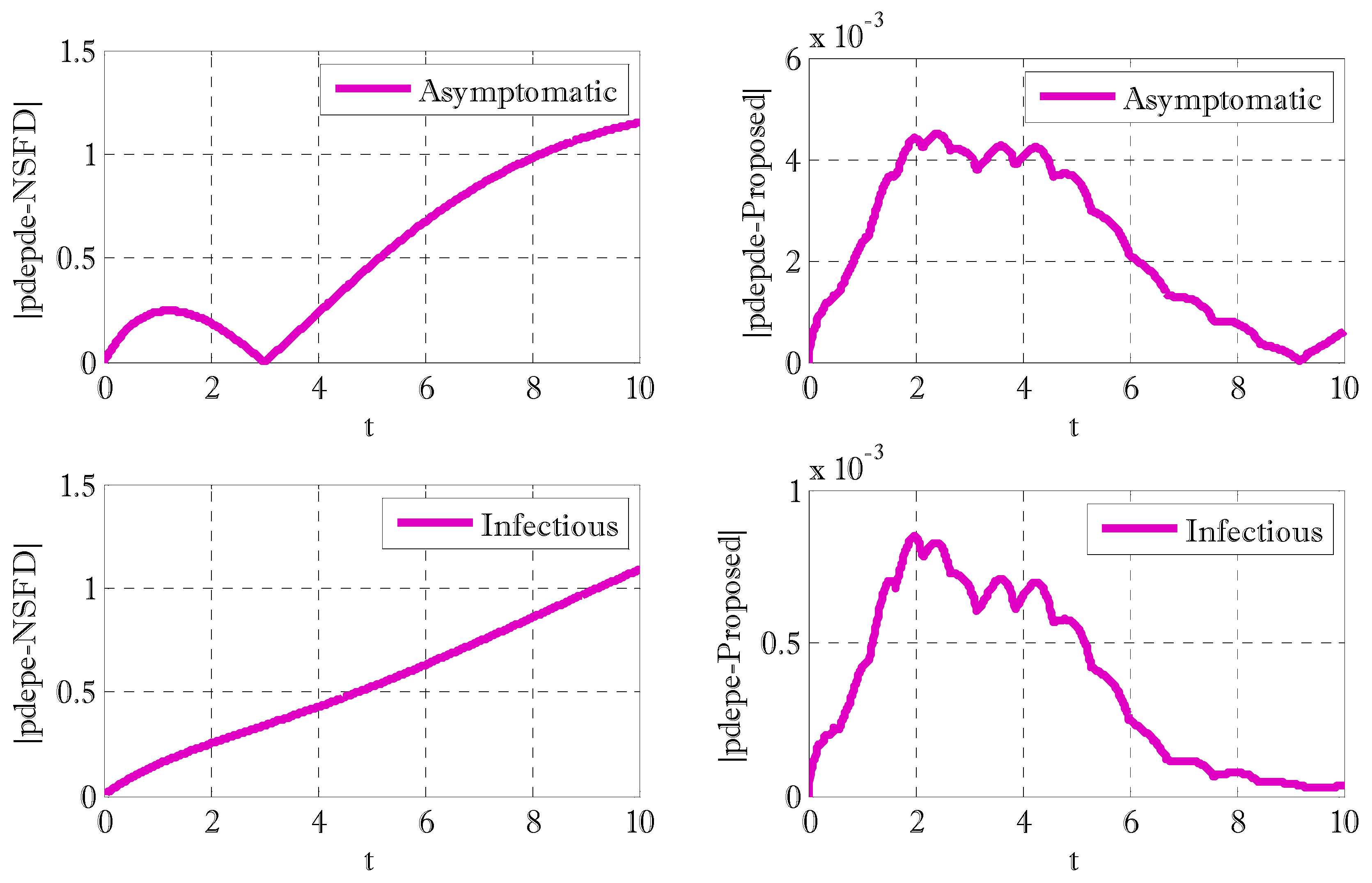
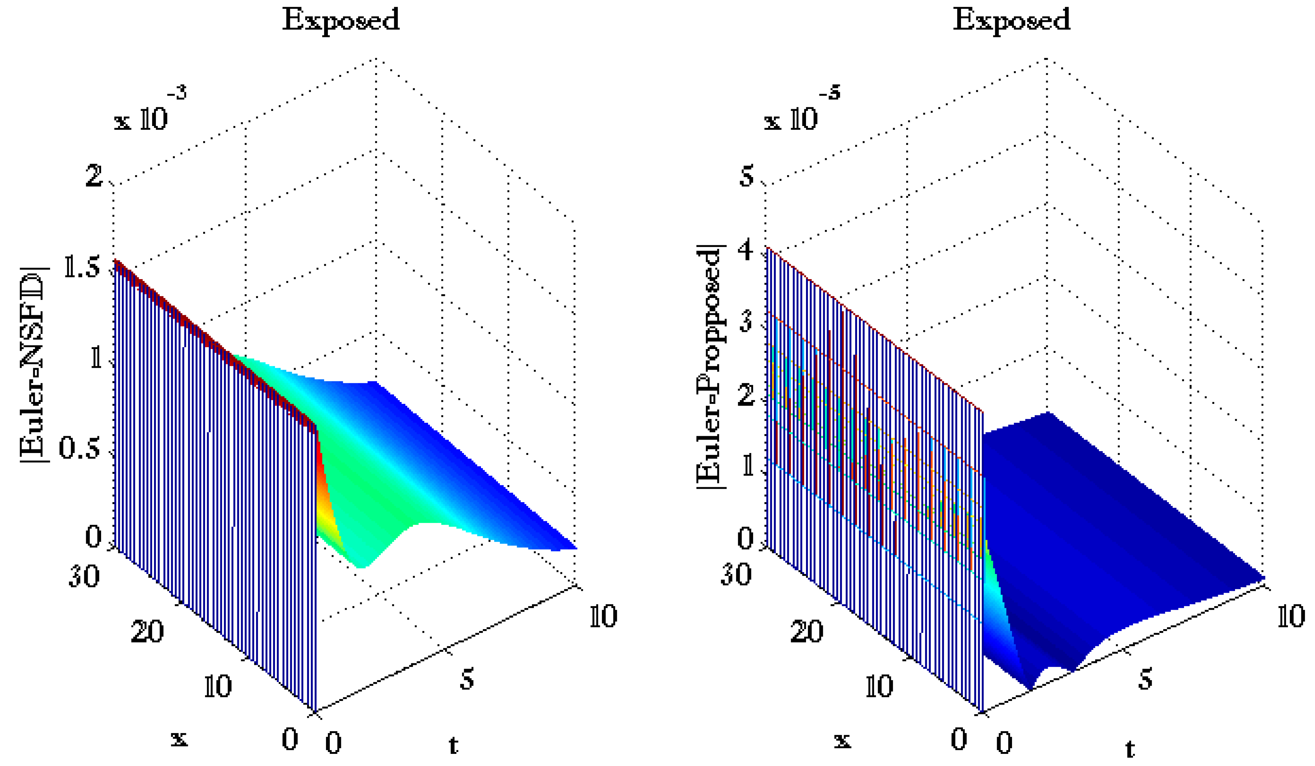
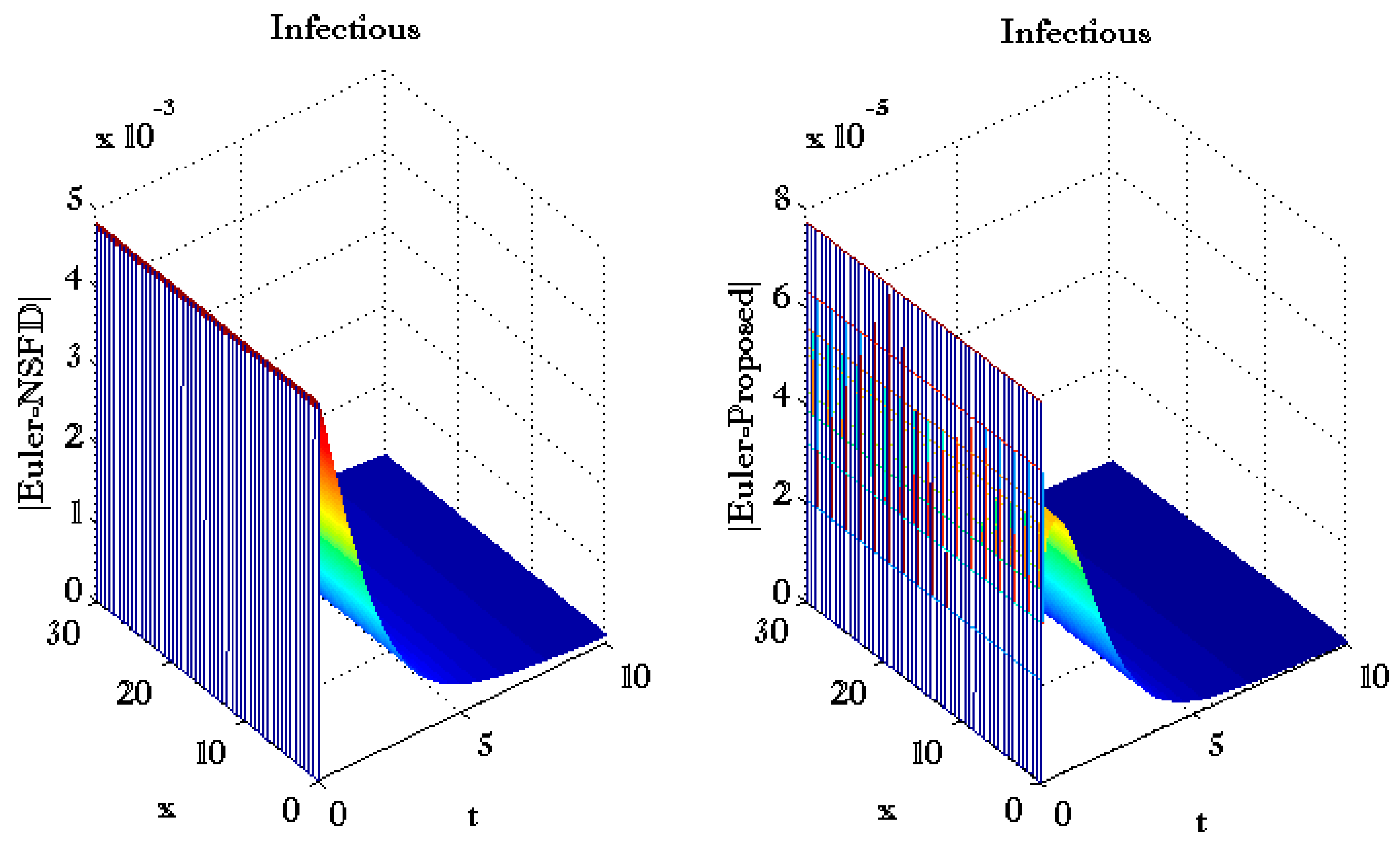
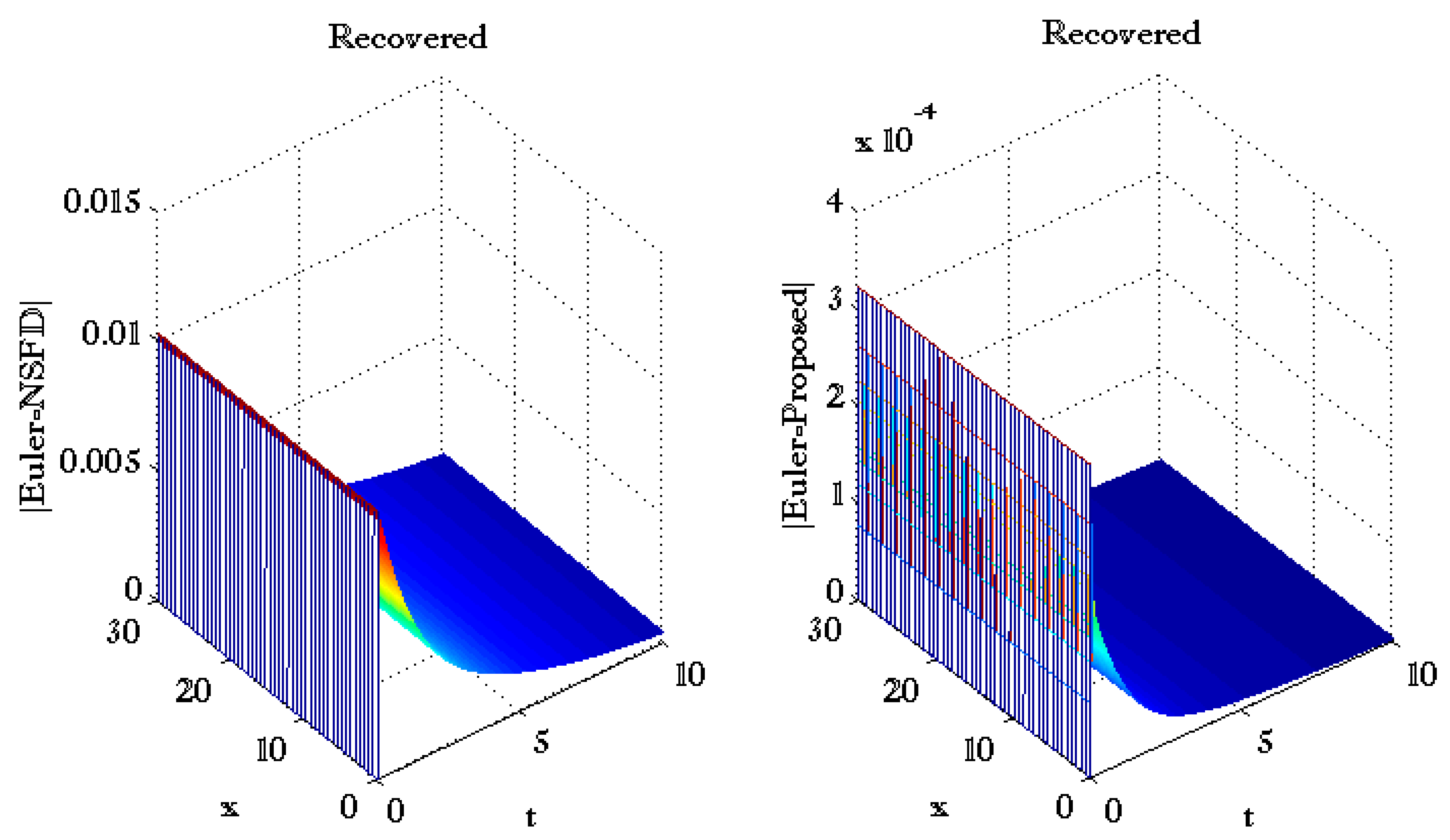
In Equation (78), k in the superscript is used for the iteration number. Since an initial guess is chosen at the first iteration, the information of the chosen initial guess will be used to find susceptible individuals at the first grid point. These iterations will continue until the stopping criteria are met. The stopping criteria are based on the norm of the difference between solutions computed on two consecutive iterations. When the norms of each equation are less than some given smaller value close to zero, the iterations will be stopped, and the final solution will be obtained. Figure 1, Figure 2 and Figure 3 show the comparison of the proposed and non-standard finite difference methods. The scheme will be more accurate if the absolute error in Figure 1, Figure 2 and Figure 3 is near zero. The proposed scheme produced a smaller error as compared to NSFD over time with an integer-order time derivative. The error is determined by finding the absolute difference between the solutions obtained by NSFD/proposed scheme and MATLAB built-in solver pdepe. For non-integer time derivatives, the comparison is made with the first-order fractional forward Euler method. The three-dimensional error plots are given in Figure 4, Figure 5, Figure 6, Figure 7 and Figure 8. Again, the scheme will be more accurate if the absolute error is less than the absolute error produced by the other scheme. From Figure 4, Figure 5, Figure 6, Figure 7 and Figure 8, it can be seen that the proposed fractional numerical scheme is more accurate than the fractional non-standard finite difference method. Moreover, these results are numerical evidence that the non-standard finite difference method considered in this work is not first-order accurate.
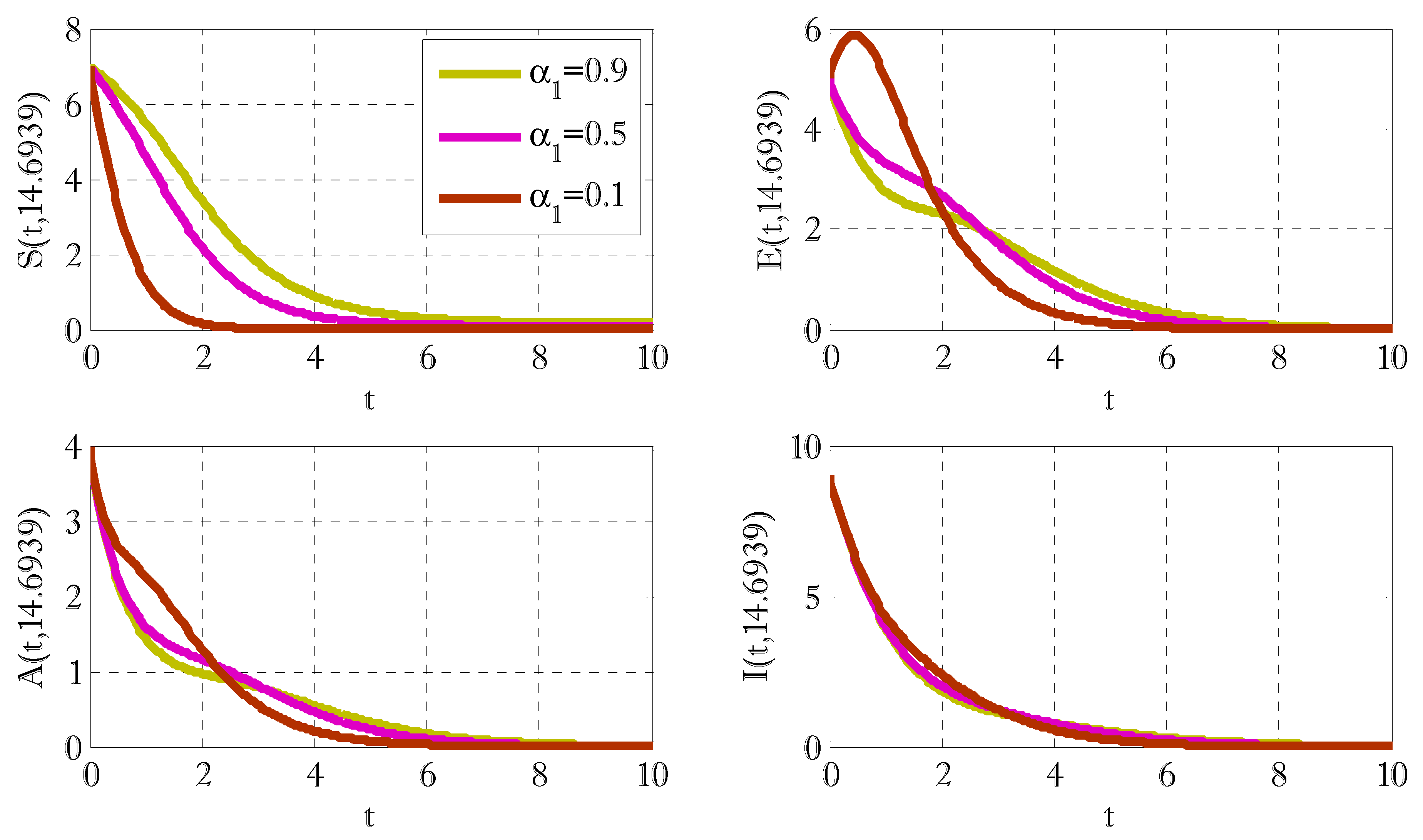
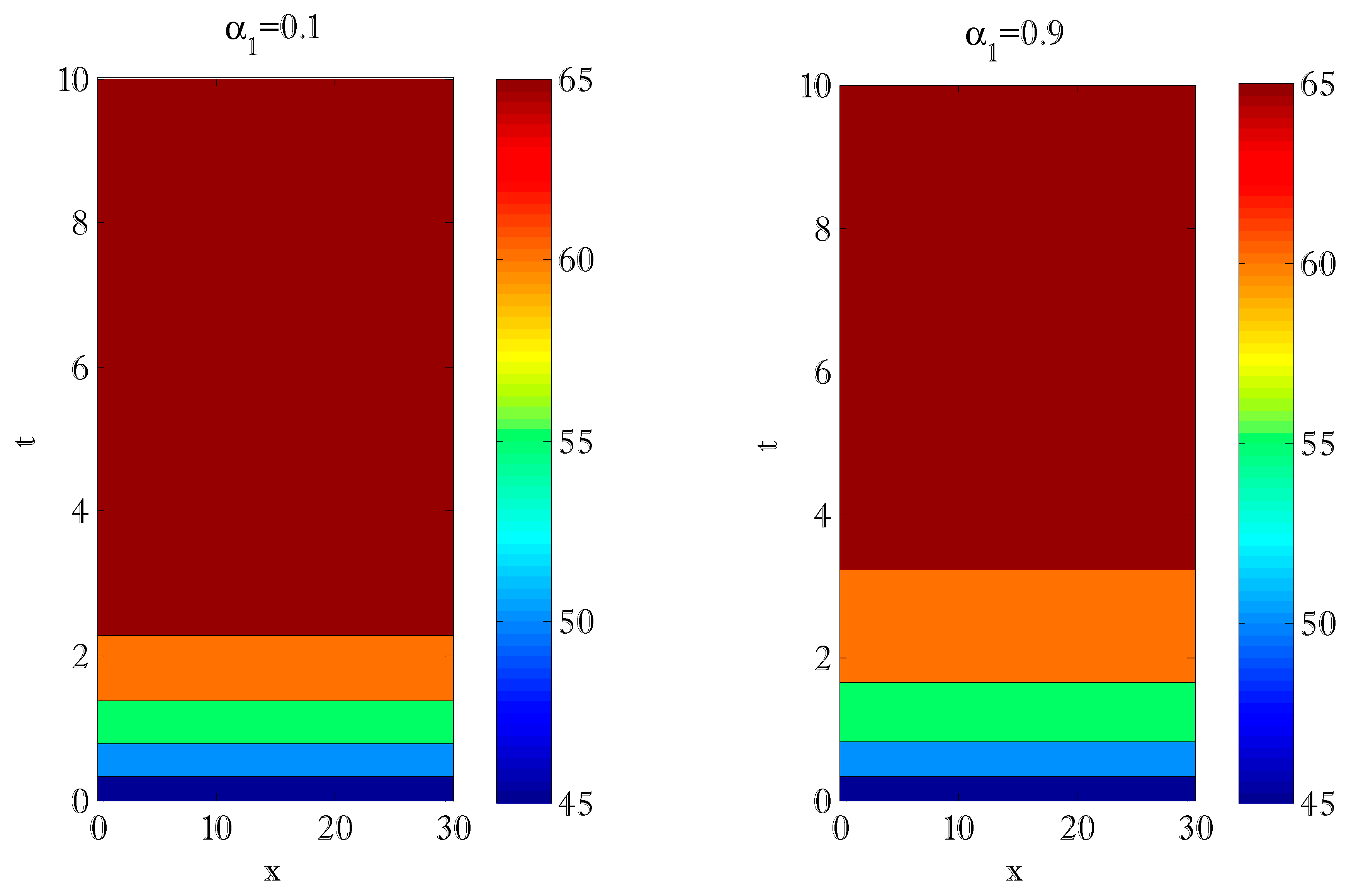
Figure 9 compares the impact of the bilinear incidence rate parameter α 1 on susceptible, exposed, asymptomatic, and infectious individuals. This figure shows that susceptible individuals de-escalate by increasing values of bilinear incidence rate, and exposed, asymptomatic, and infectious people have both increasing and decreasing behavior. These three categories of people have increasing behavior for the first interval of time, and then this behavior is reversed. Figure 10 shows the contour plots for recovered people by varying bilinear incidence rate parameters. The difference between both contour plots can be seen in this figure. Figure 11 shows the impact of fractional parameter α on four categories of people. Clearly, Figure 11 shows the increasing behavior of susceptible, exposed, asymptomatic, and infectious people by enhancing the values of the fractional parameter. By increasing the order of fractional time derivatives, a growth in four categories of people can be seen. Figure 12 shows the impact of fractional parameters on recovered people in the form of contours.
Table 1 shows the comparison of the proposed scheme with the nonstandard finite difference method for the integer-order time derivative. The errors produced by both schemes can be seen in this table. The error is found when the norm of the difference of two solutions is computed. Both schemes are checked when their comparison is made with MATLAB solver pdepe. The higher norm of error shows the higher error in the solution. In Figure 9 and Figure 11, L denotes the length of the boundary. Figure 9 and Figure 11 are drawn at a fixed value of x = 14.6939 and in Table 1, Nx = 50, and Nt = 300 denote the number of grid points and the number of time levels respectively.
It is to be noted that the values of parameters are chosen randomly and are somewhat suitable for the comparison of the two schemes.

4. Conclusions

In this work, a fractional numerical scheme is proposed to solve fractional time-dependent problems. A modified model of the diffusive epidemic model was constructed with a non-linear incidence rate. The proposed scheme was second-order accurate in space. The stability of the fractional numerical scheme has been given, and convergence conditions have also been found. It was also pointed out that the fractional non-standard finite difference method is not accurate enough to use in its present form. The performance of the proposed scheme was also checked by comparing the results with the MATLAB built-in solver pdepe for the classical case. This comparison showed the accuracy of the proposed scheme and described the inaccuracy of the considered form of the nonstandard finite difference method for problems with diffusion effects. The proposed fractional numerical scheme can be used in situations where the conditions of obtaining a positive solution are desired with unconditional stability for numerous problems in science and engineering. As a result of the completion of this study, it is feasible to propose further applications for the currently available approach [34,35,36].

Author Contributions

Conceptualization, Y.N.; Funding acquisition, W.S.; Investigation, Methodology, Software, Formal Analysis, Writing—review and editing, Y.N.; Methodology, M.S.A.; Project administration, W.S.; Resources, W.S.; Supervision, M.S.A.; Visualization, W.S.; Writing—original draft, M.S.A. All authors have read and agreed to the published version of the manuscript.

Funding

The authors would like to acknowledge the support of Prince Sultan University for paying the Article Processing Charges (APC) of this publication.

Institutional Review Board Statement

Not applicable.

Informed Consent Statement

Not applicable.

Data Availability Statement

The manuscript includes all required data and implementing information.

Acknowledgments

We warmly thank the anonymous referees. The second and third authors wish to express their gratitude to Prince Sultan University for facilitating the publication of this article through the Theoretical and Applied Sciences Lab.

Conflicts of Interest

The authors declare no conflict of interest.

References

  1. World Health Organization (WHO). 2019. Available online: https://www.who.int/ (accessed on 29 April 2021).
  2. Kermack, W.O.; McKendrick, A.G. A contribution to the mathematical theory of epidemics. Proc. R. Soc. Lond. Ser. Math. Phys. Sci. 1927, 115, 700–721. [Google Scholar] [CrossRef] [Green Version]
  3. Hethcote, H.W. The Mathematics of Infectious Diseases. SIAM Rev. 2000, 42, 599–653. [Google Scholar] [CrossRef] [Green Version]
  4. Brauer, F. Mathematical epidemiology: Past, present, and future. Infect. Dis. Model. 2017, 2, 113–127. [Google Scholar] [CrossRef] [PubMed]
  5. Atangana, A.; Alkahtani, B.S.T. Analysis of the Keller–Segel Model with a Fractional Derivative without Singular Kernel. Entropy 2015, 17, 4439–4453. [Google Scholar] [CrossRef]
  6. Thabet, S.T.; Abdo, M.S.; Shah, K.; Abdeljawad, T. Study of transmission dynamics of COVID-19 mathematical model under ABC fractional order derivative. Results Phys. 2020, 19, 103507. [Google Scholar] [CrossRef]
  7. Atangana, A.; Baleanu, D. New fractional derivatives with nonlocal and non-singular kernel: Theory and application to heat transfer model. Therm. Sci. 2016, 20, 763–769. [Google Scholar] [CrossRef] [Green Version]
  8. Atangana, A.; Koca, I. On the new fractional derivative and application to nonlinear Baggs and Freedman model. J. Nonlinear Sci. Appl. 2016, 9, 2467–2480. [Google Scholar] [CrossRef] [Green Version]
  9. Khan, M.A.; Atangana, A. Modeling the dynamics of novel coronavirus (2019-nCov) with fractional derivative. Alex. Eng. J. 2020, 59, 2379–2389. [Google Scholar] [CrossRef]
  10. Ullah, M.Z.; Alzahrani, A.K.; Baleanu, D. An efficient numerical technique for a new fractional tuberculosis model with nonsingular derivative operator. J. Taibah Univ. Sci. 2019, 13, 1147–1157. [Google Scholar] [CrossRef]
  11. Oluyori, D.A.; Adebayo, H.O.; Pérez, A.G.C. Global analysis of an SEIRS model for COVID-19 capturing saturated incidence with treatment response. Appl. Appl. Math. 2021, 16, 924–925. [Google Scholar]
  12. Okhuese, A.V. Estimation of the probability of reinfection with COVID-19 by the susceptible-exposed infectious-removed-undetectable-susceptible model. JMIR Public Health Surveill. 2020, 6, e19097. [Google Scholar] [CrossRef]
  13. Okhuese, A.V. Mathematical predictions for COVID-19 as a global pandemic. SSRN. 2020, p. 3555879, Preprint. Available online: https://ssrn.com/abstract=3555879 (accessed on 15 December 2021).
  14. Malkov, E. Simulation of coronavirus disease 2019 (COVID-19) scenarios with ossibility of reinfection. Chaos Solitons Fractals 2020, 139, 110296. [Google Scholar] [CrossRef] [PubMed]
  15. Mohd, M.H.; Sulayman, F. Unravelling the myths of R0 in controlling the dynamics of COVID-19 outbreak: A modelling perspective. Chaos Solitons Fractals 2020, 138, 109943. [Google Scholar] [CrossRef] [PubMed]
  16. Fichet-Calvet, E.; Rogers, D.J. Risk Maps of Lassa Fever in West Africa. PLOS Negl. Trop. Dis. 2009, 3, e388. [Google Scholar] [CrossRef]
  17. Bausch, D.G.; Schwarz, L. Outbreak of Ebola Virus Disease in Guinea: Where Ecology Meets Economy. PLoS Negl. Trop. Dis. 2014, 8, e3056. [Google Scholar] [CrossRef] [PubMed]
  18. Gumel, A.B.; McCluskey, C.C.; Watmough, J. An SVEIR model for assessing potential impact of an imperfectanti-SARS vaccine. Math. Biosci. Eng. 2006, 3, 485–512. [Google Scholar] [PubMed]
  19. Liu, X.; Takeuchi, Y.; Iwami, S. SVIR epidemic models with vaccination strategies. J. Theor. Biol. 2008, 253, 1–11. [Google Scholar] [CrossRef]
  20. Wei, H.; Jiang, Y.; Song, X.; Su, G.; Qiu, S. Global attractivity and permanence of a SVEIR epidemic model with pulse vaccination and time delay. J. Comput. Appl. Math. 2009, 229, 302–312. [Google Scholar] [CrossRef] [Green Version]
  21. Cai, L.-M.; Li, Z.; Song, X. Global analysis of an epidemic model with vaccination. J. Appl. Math. Comput. 2018, 57, 605–628. [Google Scholar] [CrossRef]
  22. Alexander, M.E.; Bowman, C.; Moghadas, S.M.; Summers, R.; Gumel, A.B.; Sahai, B.M. A vaccination model for transmission dynamics of influenza. SIAM J. Appl. Dyn. Syst. 2004, 3, 503–524. [Google Scholar] [CrossRef]
  23. Arino, J.; McCluskey, C.C.; Driessche, P.V.D. Global Results for an Epidemic Model with Vaccination that Exhibits Backward Bifurcation. SIAM J. Appl. Math. 2003, 64, 260–276. [Google Scholar] [CrossRef] [Green Version]
  24. Aldila, D. Cost-effectiveness and backward bifurcation analysis on COVID-19 transmission model considering direct and indirect transmission. Commun. Math. Biol. Neurosci. 2020, 2020, 49. [Google Scholar] [CrossRef]
  25. Aldila, D.; Khoshnaw, S.H.A.; Safitri, E.; Anwar, Y.R.; Bakry, A.R.Q.; Samiadji, B.M.; Anugerah, D.A.; Alfarizi, M.F.; Ayulani, I.D.; Salim, S.N. A mathematical study on the spread of COVID-19 considering social distancing and rapid assessment: The case of Jakarta, Indonesia. Chaos Solitons Fractals 2020, 139, 110042. [Google Scholar] [CrossRef] [PubMed]
  26. Daşbaşı, B. Stability Analysis of an Incommensurate Fractional-Order SIR Model. Math. Model. Numer. Simul. Appl. 2021, 1, 44–55. [Google Scholar] [CrossRef]
  27. Özköse, F.; Şenel, M.T.; Habbireeh, R. Fractional-order mathematical modelling of cancer cells-cancer stem cells-immune system interaction with chemotherapy. Math. Model. Numer. Simul. Appl. 2021, 1, 67–83. [Google Scholar] [CrossRef]
  28. Ikram, R.; Khan, A.; Zahri, M.; Saeed, A.; Yavuz, M.; Kumam, P. Extinction and stationary distribution of a stochastic COVID-19 epidemic model with time-delay. Comput. Biol. Med. 2021, 141, 105115. [Google Scholar] [CrossRef] [PubMed]
  29. Vahid RezaHosseini, W.-Z. The numerical solution of high dimensional variable-order time fractional diffusion equation via the singular boundary method. J. Adv. Res. 2021, 32, 73–84. [Google Scholar]
  30. Nikan, O.; Avazzadeh, Z. An improved localized radial basis-pseudospectral method for solving fractional reaction–subdiffusion problem. Results Phys. 2021, 23, 104048. [Google Scholar] [CrossRef]
  31. Aghdam, Y.E.; Khoshkhahtinat, M. High-accuracy numerical scheme for solving the space-time fractional advection-diffusion equation with convergence analysis. Alex. Eng. J. 2022, 61, 217–225. [Google Scholar] [CrossRef]
  32. Podlubny, I. Fractional Differential Equations; Academic Press: San Diego, CA, USA, 1999. [Google Scholar]
  33. Usero, D. Fractional Taylor Series for Caputo Fractional Derivatives, Construction of Numerical Schemes, Preprint. Available online: http://www.fdi.ucm.es/profesor/vazquez (accessed on 10 November 2021).
  34. Nawaz, Y.; Arif, M.S.; Ashraf, M.U. Development of Explicit Schemes for Diffusive SEAIR COVID-19 Epidemic Spreading Model: An Application to Computational Biology. Iran. J. Sci. Technol. Trans. A Sci. 2021, 45, 2109–2119. [Google Scholar] [CrossRef]
  35. Nawaz, Y.; Arif, M.S.; Bibi, M.; Abbasi, J.N.; Javed, U.; Nazeer, A. A finite difference method and effective modification of gradient descent optimization algorithm for MHD fluid flow over a linearly stretching surface. Comput. Mater. Contin. 2020, 62, 657–677. [Google Scholar] [CrossRef]
  36. Nawaz, Y.; Arif, M.; Shatanawi, W.; Nazeer, A. An Explicit Fourth-Order Compact Numerical Scheme for Heat Transfer of Boundary Layer Flow. Energies 2021, 14, 3396. [Google Scholar] [CrossRef]
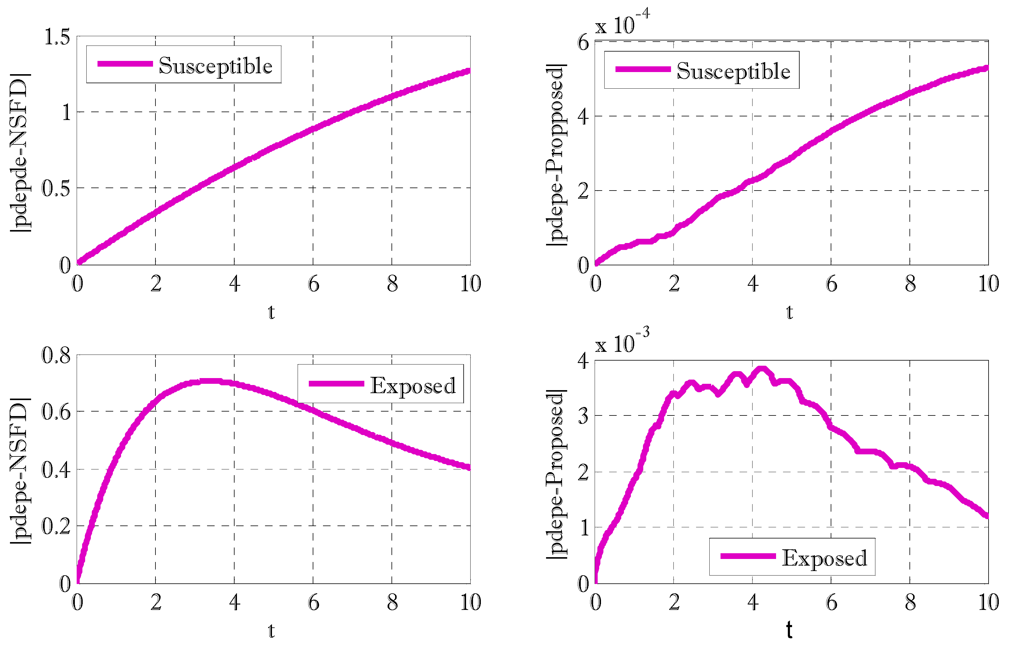
Figure 1. Two-dimensional comparison of proposed and NSFD schemes for susceptible and exposed individuals using L = 10 , N x = 50 , N t = 700 , α 1 = 0.5 , β = 0.3 , γ = 0.4 , σ = 0.1 , μ = 0.1 , d 1 = d 2 = d 3 = d 4 = d 5 = 0.9 , α = 1 .
Fractalfract 06 00078 g001
Figure 2. Two-dimensional comparison of proposed and NSFD schemes for asymptomatic and infectious individuals using L = 10 , N x = 50 , N t = 700 , α 1 = 0.5 , β = 0.3 , γ = 0.4 , σ = 0.1 , μ = 0.1 , d 1 = d 2 = d 3 = d 4 = d 5 = 0.9 , α = 1 .
Fractalfract 06 00078 g002
Figure 3. Two-dimensional comparison of proposed and NSFD schemes for recovered individuals using L = 10 , N x = 50 , N t = 700 , α 1 = 0.5 , β = 0.3 , γ = 0.4 , σ = 0.1 , μ = 0.1 , d 1 = d 2 = d 3 = d 4 = d 5 = 0.9 , α = 1 .
Fractalfract 06 00078 g003
Figure 4. Three-dimensional comparisons of proposed and NSFD schemes for susceptible individuals using N x = 50 , N t = 1300 , α 1 = 0.1 , β = 0.1 , γ = 0.3 , σ = 0.4 , μ = 0.5 , d 1 = 2 , d 2 = 2.5 , d 3 = 2.5 , d 4 = 2 , d 5 = 2 , α = 0.9 .
Fractalfract 06 00078 g004
Figure 5. Three-dimensional comparisons of proposed and NSFD schemes for exposed individuals using N x = 50 , N t = 1300 , α 1 = 0.1 , β = 0.1 , γ = 0.3 , σ = 0.4 , μ = 0.5 , d 1 = 2 , d 2 = 2.5 , d 3 = 2.5 , d 4 = 2 , d 5 = 2 , α = 0.9 .
Fractalfract 06 00078 g005
Figure 6. Three-dimensional comparisons of proposed and NSFD schemes for asymptomatic individuals using N x = 50 ,   N t = 1300 , α 1 = 0.1 , β = 0.1 , γ = 0.3 , σ = 0.4 , μ = 0.5 , d 1 = 2 , d 2 = 2.5 , d 3 = 2.5 , d 4 = 2 , d 5 = 2 , α = 0.9 .
Fractalfract 06 00078 g006
Figure 7. Three-dimensional comparisons of proposed and NSFD schemes for infectious individuals using N x = 50 , N t = 1300 , α 1 = 0.1 , β = 0.1 , γ = 0.3 , σ = 0.4 , μ = 0.5 , d 1 = 2 , d 2 = 2.5 , d 3 = 2.5 , d 4 = 2 , d 5 = 2 , α = 0.9 .
Fractalfract 06 00078 g007
Figure 8. Three-dimensional comparisons of proposed and NSFD schemes for recovered individuals using N x = 50 , N t = 1300 , α 1 = 0.1 , β = 0.1 , γ = 0.3 , σ = 0.4 , μ = 0.5 , d 1 = 2 , d 2 = 2.5 , d 3 = 2.5 , d 4 = 2 , d 5 = 2 , α = 0.9 .
Fractalfract 06 00078 g008
Figure 9. Impact of the bilinear incidence rate parameter α 1 on susceptible, exposed, asymptomatic, and infected individuals using N x = 50 , N t = 300 , β = 0.9 , γ = 0.7 , σ = 0.9 , μ = 0.9 , d 1 = 2 , d 2 = 2.5 , d 3 = 2.5 , d 4 = 2 , d 5 = 2 , α = 0.9 , L = 30 .
Fractalfract 06 00078 g009
Figure 10. Impact of the bilinear incidence rate parameter α 1 on recovered individuals using N x = 50 , N t = 300 , β = 0.9 , γ = 0.7 , σ = 0.9 , μ = 0.9 , d 1 = 2 , d 2 = 2.5 , d 3 = 2.5 , d 4 = 2 , d 5 = 2 , α = 0.9 .
Fractalfract 06 00078 g010
Figure 11. Impact of fractional order parameter α on susceptible, exposed, asymptomatic, and infected individuals using N x = 50 , N t = 300 , α 1 = 0.9 , β = 0.9 , γ = 0.7 , σ = 0.9 , μ = 0.9 , d 1 = 2 , d 2 = 2.5 , d 3 = 2.5 , d 4 = 2 , d 5 = 2 , L = 30 .
Fractalfract 06 00078 g011
Figure 12. Impact of fractional order parameter α on recovered individuals using N x = 50 , N t = 300 , α 1 = 0.9 , β = 0.9 , γ = 0.7 , σ = 0.9 , μ = 0.9 , d 1 = 2 , d 2 = 2.5 , d 3 = 2.5 , d 4 = 2 , d 5 = 2 , α = 0.9 .
Fractalfract 06 00078 g012
Table 1. Comparison of proposed and NSFD schemes over spatial coordinate x using d1 = 2, d2 = 2.5, d3 = 2.5, d4 = 2, d5 = 2, Nx = 50, and Nt = 300.
β Norm of Error
α 1 γ σ μ ProposedNSFD
0.10.10.30.40.57.3001 × 10−43.3566
0.9 0.00604.3839
0.9 0.01283.8177
0.7 0.01474.3007
0.9 0.02045.5968
0.90.00991.7447
Publisher’s Note: MDPI stays neutral with regard to jurisdictional claims in published maps and institutional affiliations.