Abstract
Contact problems are among the most difficult issues in mathematics and are of crucial practical importance in engineering applications. This paper presents a scaled boundary finite-element method with B-differentiable equations for 3D frictional contact problems with small deformation in elastostatics. Only the boundaries of the contact system are discretized into surface elements by the scaled boundary finite-element method. The dimension of the contact system is reduced by one. The frictional contact conditions are formulated as B-differentiable equations. The B-differentiable Newton method is used to solve the governing equation of 3D frictional contact problems. The convergence of the B-differentiable Newton method is proven by the theory of mathematical programming. The two-block contact problem and the multiblock contact problem verify the effectiveness of the proposed method for 3D frictional contact problems. The arch-dam transverse joint contact problem shows that the proposed method can solve practical engineering problems. Numerical examples show that the proposed method is a feasible and effective solution for frictional contact problems.
1. Introduction
Contact problems are among the most difficult issues in mechanics and are of crucial practical importance in engineering applications. The main difficulty lies in their nonlinearity, which is caused when the contact region and the contact status are unknown, and the contact conditions are unilateral inequality constraints. It is difficult to obtain accurate solutions by simulating real contact systems with mathematical models for complex contact problems in practical engineering. Thus, numerical methods have been widely used to analyze contact problems. The finite-element method [1,2,3,4,5], as the most commonly used numerical method, has been widely employed to solve contact problems. The FEM needs to discretize the full domain of the contact problem, which will increase the calculation amount. The boundary element method [6,7] only discretizes the boundary of the contact body, which reduces the dimension of the original problem. However, it is difficult to determine the fundamental solution for a complex region. As a new numerical method, isogeometric analysis [8,9,10,11] realizes the seamless connection between CAD and CAE, solves the inconsistency problem between the geometric model and the computational model in traditional numerical methods, and can accurately describe the geometric boundary of the computational domain. Like in the FEM, the IGA also needs to discretize the whole computational domain.
The key problem in contact analysis is determining the size of the contact area and the distribution of contact pressure, which mainly focuses on the boundary of the problem. The scaled boundary finite-element method [12,13] is a semi-analytical numerical method that only discretizes the outer boundary of the computational domain, reduces the problem dimension by one, accurately simulates the infinite domain, and does not need a fundamental solution. The SBFEM has been widely used in the fields of fracture mechanics [14,15,16], seepage problems [17,18,19], dam–reservoir interactions [20,21] and contact problems [22,23,24,25,26].
Another key problem in contact analysis is how to enforce the contact constraint conditions. The penalty function method [1,27], Lagrange multiplier method [5,24,28], augmented Lagrange multiplier method [29] and mathematical programming method [3,4,22,30] are often used to treat contact constraint conditions. The penalty function method is an approximate method, which allows the contact bodies to embed with each other. The selection of the penalty factor has great influence on the accuracy and convergence of the results. The Lagrange multiplier method can accurately simulate contact conditions, and the Lagrange multiplier has a certain mechanical significance in terms of contact force. The augmented Lagrange multiplier method improves the convergence by introducing higher penalty factors. When the penalty function method, the Lagrange multiplier method or the augmented Lagrange multiplier method is used to enforce the contact constraint conditions, and the classical Newton–Raphson method is often used in contact iterative calculations. The total function of the contact system is nonsmooth due to the existence of contact forces. Thus, the convergence is difficult to guarantee in the classical Newton–Raphson method. The mathematical programming method has a strict mathematical theoretical basis [31]. The B-differentiable equations (BDEs) method [2], as one of the mathematical programming methods, can accurately impose the contact constraint conditions, which are initiated from the augmented Lagrange approach [32]. The B-differentiable equations can be solved by the B-differentiable Newton method [33], which uses global convergence under some mild assumptions. Thus, the SBFEM with BDEs has been used to solve 2D frictionless contact problems [22], and the effectiveness and accuracy of the SBFEM with BDEs method have been verified by some examples.
This paper presents an extension of the SBFEM with BDEs to 3D frictional contact problems with small deformation in elastostatics. In the framework of the SBFEM–BDEs, the contact body is discretized by using the SBFEM, and the frictional contact conditions are enforced by BDEs. The B-differentiable Newton method is used to solve the governing equation of 3D frictional contact problems. The convergence of the B-differentiable Newton method is proved by the theory of mathematical programming.
The following sections of this paper are organized as follows: the frictional contact conditions of 3D problems are introduced in Section 2. In Section 3, the discretization scheme for a 3D bounded domain based on the SBFEM is summarized. The governing equations of the 3D frictional contact problems based on the SBFEM with BDEs, and their solutions, are derived in Section 4. The effectiveness of the SBFEM with BDEs is verified by numerical examples in Section 5. Some conclusions are presented in Section 6.
2. Frictional Contact Formulations
For simplicity, a contact system includes two contact bodies Ωi (i = 1, 2), as shown in Figure 1. Each contact body is within the range of small elastostatic deformation. The gap between the contact surfaces is very small compared with the size of the contact body. Thus, the contact conditions can be judged and applied by a node-to-node scheme. , and (i = 1, 2) mean the given Dirichlet boundary, the given Neumann boundary and the potential contact boundary, respectively. For the contact system, , , . The superscript i (i = 1,2) denotes the variables belong to each contact body. When the variables are suitable for the contact system, the superscript i can be omitted. A local coordinate system nab is defined on the potential contact surface.
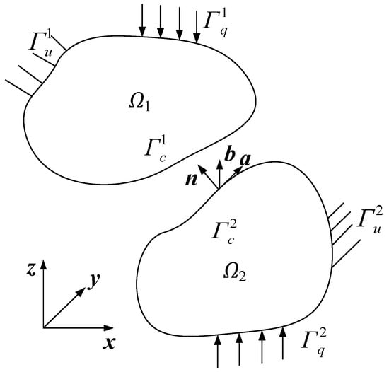
Figure 1.
A sketch of the contact problem.
The basic equations of static friction contact problems in incremental form can be expressed as:
with the Neumann and Dirichlet boundary conditions:
where , and mean the stress increment, strain increment and displacement increment, respectively; means the body load increment; means the given stress increment; means the given displacement increment; means the elastic matrix; and means the outward unit vector. The incremental formulations are the increments within a time evolution of the deformed state of both bodies.
The friction contact conditions on the potential contact boundary are:
- (1)
- The contact pressures on the two contact surfaces are equal in magnitude and opposite in direction.
- (2)
- In the normal direction, the contact pressures are assumed to be compressive and the contact surfaces cannot be embedded within each other.
- Opening:
- Bonding:
- (3)
- The tangential friction contact condition satisfies Coulomb’s friction law:
- Opening:
- Bonding:
The governing equations, Equations (1)–(3), and boundary conditions (4)–(10) constitute the frictional contact formulations of 3D problems. According to the principle of virtual work, the virtual work equation of the contact system in incremental form can be expressed as:
3. The Scaled Boundary Finite-Element Method
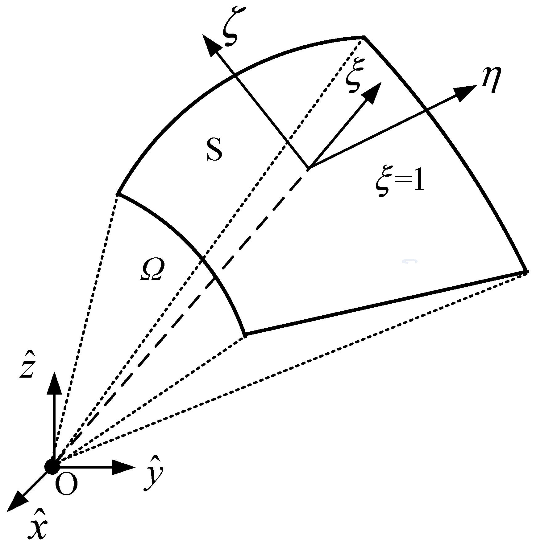
By using the SBFEM, a 3D domain is discretized into a number of subdomains or polyhedrons which satisfy the scaling requirement. The scaling requirement means that all the boundary is visible from the scaling center for each subdomain or polyhedron. Only the boundaries of subdomains or polyhedrons are discretized with surface elements. Figure 2 illustrates a typical surface element S with four nodes of a section of subdomain Ω. To describe the inner domain of Ω, a scaled boundary coordinate system is established, which consists of a dimensionless radial coordinate and local coordinates . The radial coordinate from the scaling center O to the boundary is defined in the radial direction, with at the scaling center O and at the boundary. The local coordinates vary from −1 to 1. Surface elements S on the boundary are constructed as isoparametric elements in the FEM.

Figure 2.
Sketch of the scaled boundary coordinate system.
A point within domain Ω in a Cartesian coordinate system can be represented using the scaled boundary coordinates :
where are Cartesian coordinates of the scaling center, are Cartesian coordinates of a point on the boundary , are the nodal coordinates of the surface element in Cartesian coordinates, and is the shape function, which is independent of the radial coordinate .
The relationship of gradient operator in Cartesian coordinates and in the scaled boundary coordinates can be expressed as:
with
where is a Jacobian matrix on the boundary.
According to the isoparametric concept, the shape function used in the transformation of coordinates is employed in the displacement field:
where is the function of the nodal displacement increment.
Then, the strain filed and the stress field can be expressed as:
with
where ND is the number of nodes in the surface element, k = 1, 2, …, ND, and in and is the element in the inverse matrix of .
Substituting Equations (16)–(18) into Equation (11) and assembling all surface elements of a subdomain yield the displacement equations in the increment form of the SBFEM:
with
where:
E0, E1, and E2 are the coefficient matrix, which only depends on the material properties and the geometry of the domain. dP is the contact force increment.
Equation (23) is a nonhomogeneous, second-order, ordinary differential equation. When the last term in Equation (23) , Equation (23) can be transformed into a first-order ordinary differential equation by introducing a dual variable.
By introducing the dual variable , which is the internal force increment:
Then, combining Equations (23) and (26) leads to:
with
Performing an eigenvalue decomposition of Hamilton matrix Z leads to:
where is the eigenvector matrix and and are the positive and negative eigenvalues, respectively. .
The general solution of Equation (27) can be expressed as:
Rewriting Equation (31) in another form:
where are integration constants.
For a bounded domain, must be finite at the scaling center. Thus, the integration constant . Then, Equation (32) is simplified as:
Substituting the equation of the first row into the equation of the second row in Equation (33) at leads to:
where K means the stiffness matrix of the subdomain with . The global stiffness matrix can be assembled using the same scheme as in the FEM.
Equation (34) is an algebraic equation at boundary, which includes the unknown variables du and dP. Thus, solving Equation (34) requires supplementing the friction contact conditions. We resort to a finite step approach, through which the entire evolution of the structural response can be analyzed as a sequence of incremental problems. Only a change in configuration from a previously known state due to a finite increment of the load step is considered.
4. The B-Differentiable Equations
4.1. The Frictional Contact Conditions in BDEs Form
The definition of B-differentiable [32]: A function H: Rn →Rm is said to be B-differentiable at a point z if there exists a function BH(z): Rn →Rm, called the B-derivative of H at z, which is positively homogeneous of degree 1 (i.e., BH(z)(λv) = λBH(z)v for all v∈Rn and all λ ≥ 0), such that: .
If H is B-differentiable at all points in a set S, then H is said to be B-differentiable in S.
Based on the discretization of the contact system using the SBFEM, the frictional contact conditions (6)–(10) can be expressed as B-differentiable equations [2,3].
with
where the operator min is B-differentiable, r is a positive real number, and means the normal contact force at the ith contact pair. A contact pair consists of a node and its corresponding node on a different contact body.
The contact conditions of the contact system can be obtained by assembling the friction contact conditions of the whole contact pair:
where NC is the number of contact pairs.
Combining Equations (34) and (39) leads to:
with
Equation (40) is the governing equation of 3D frictional contact problems based on the SBFEM and BDEs, and can be solved by the B-differentiable Newton method [33]. The B-differentiable Newton method provides a descent algorithm which is globally convergent under some mild assumptions.
4.2. The B-Differentiable Newton Method
The solution of Equation (40) is transformed into an unconstrained minimization problem by using the B-differentiable Newton method, which is based on the directional derivative and line search process.
where g means the merit function.
The solution process is as follows:
Step 1. Set the number of iteration steps k = 0. Setting the convergence error ε, and constants η and δ as ε > 0, 0 < η < 1, 0 < δ < 0.5 gives the initial iteration value x0;
Step 2. Construct the search direction dxk:
where means the derivative of H at point xk in the dxk direction.
Step 3. Compute the step value of the line search:
where is the first non-negative integer l, which satisfies Equation (45).
Step 4. Compute the next iteration value xk+1:
Step 5. Detect whether xk+1 satisfies the termination criterion. If , then stop the solving process; if , then let , and return to Step 2.
The key problem is constructing the search direction dxk in the B-differentiable Newton method. The derivative of H at point xk in the dxk direction:
with
where means the gradient of H with respect to xk.
The main solution process of the SBFEM–BDEs is summarized as follows:
- Step 1: Compute the coefficient matrix E0, E1, E2 for each surface element in Equation (25);
- Step 2: Perform an eigenvalue decomposition of the Hamilton matrix Z in Equation (28);
- Step 3: Compute the stiffness matrix ;
- Step 4: Calculate du and dP by performing the solution process of the B-differentiable Newton method;
- Step 5: Compute the inner variables in the domain by solving Equation (33).
5. Numerical Examples
5.1. Two-Block Contact Problem
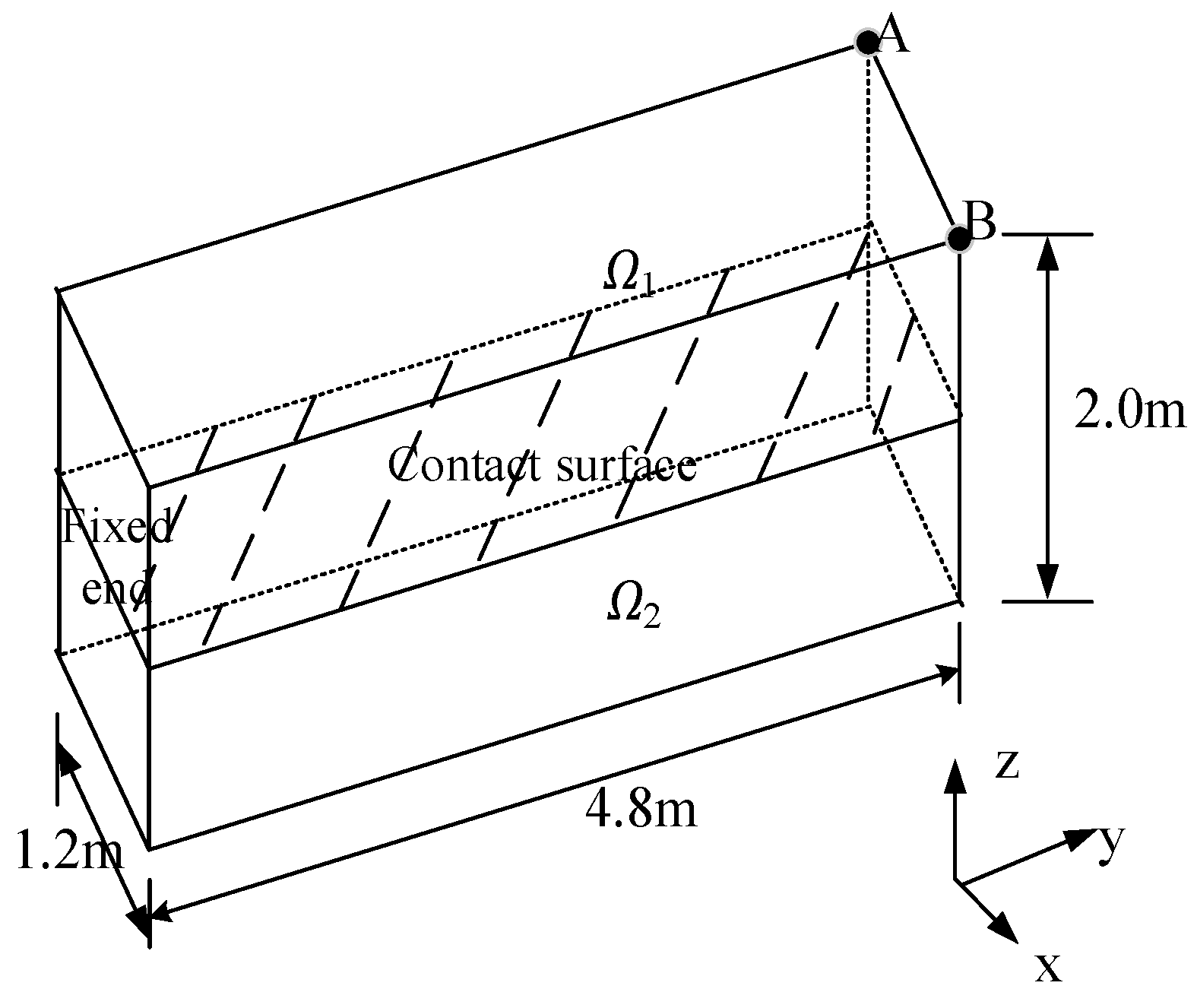
In order to verify the accuracy of the proposed method in solving 3D frictional contact problems, as shown in Figure 3, a two-block contact problem was selected for analysis. The initial gap and frictional coefficient between the two blocks are 0 and 0.5, respectively. The elasticity modulus and Poisson’s ratio of the blocks are 30 GPa and 0.3, respectively. Concentrated forces of −100 kN are simultaneously applied along the X, Y and Z directions at endpoints A and B. The left end of two blocks is fixed. There is no analytical solution for 3D frictional contact problems. Thus, the results obtained by using commercial software ANSYS are used as a reference solution.

Figure 3.
Two-block contact problem.
In ANSYS, the frictional contact constraints are enforced by the augmented Lagrange multiplier method, and the mesh densities of difference calculation models for each block are listed in Table 1. The mesh density means the number of surface/solid elements in different directions of each block. In the calculation model of the SBFEM, the mesh density of the surface element is equal to that of the solid element in the calculation model of ANSYS. As shown Figure 4, the number of DOF in the SBFEM is less than that of ANSYS with the same mesh density. This is because only the boundaries of each block need to be discretized by using the SBFEM.

Table 1.
The mesh density in different directions of each block.
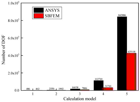
Figure 4.
Number of DOF vs. calculation model.
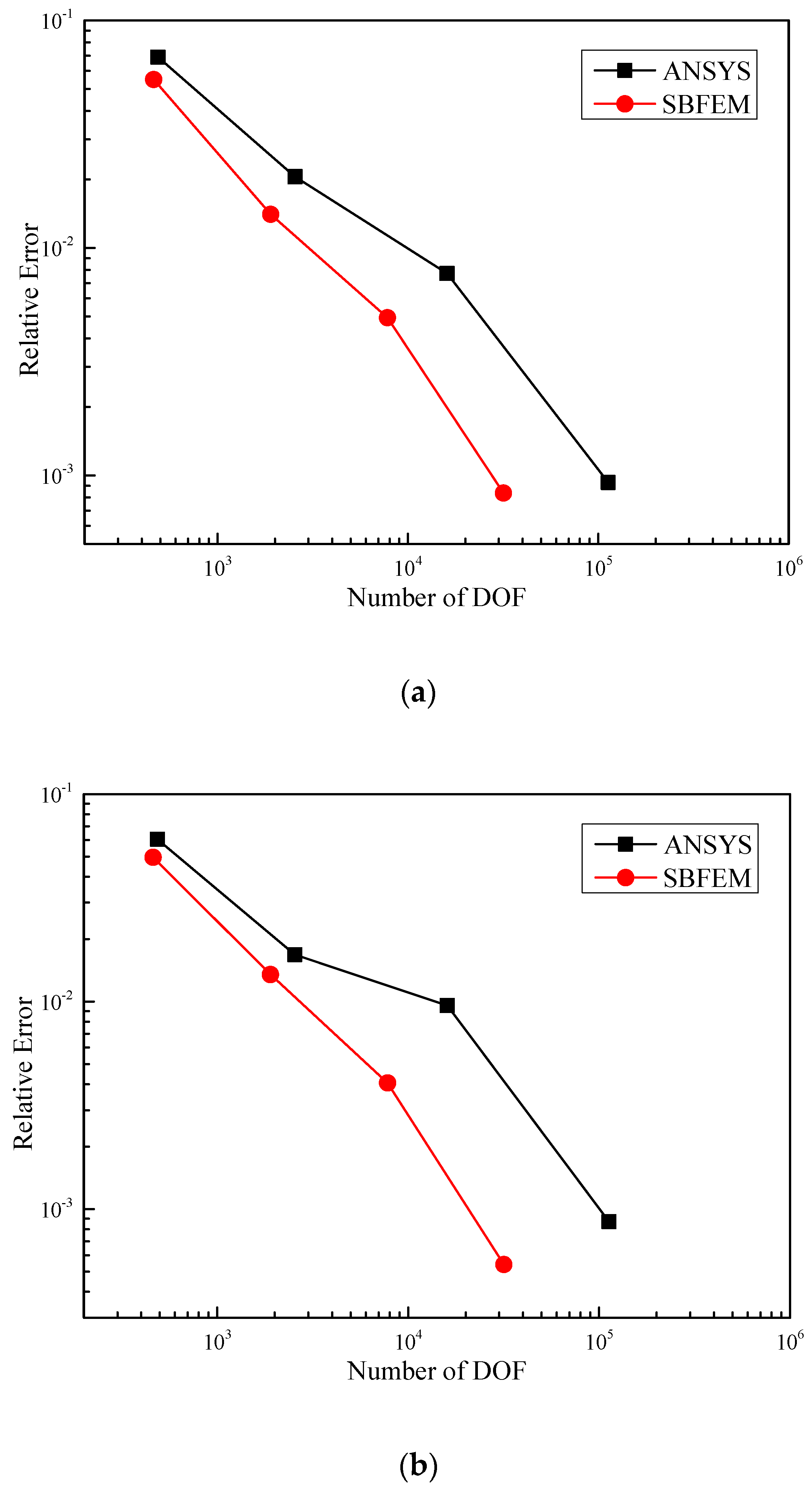
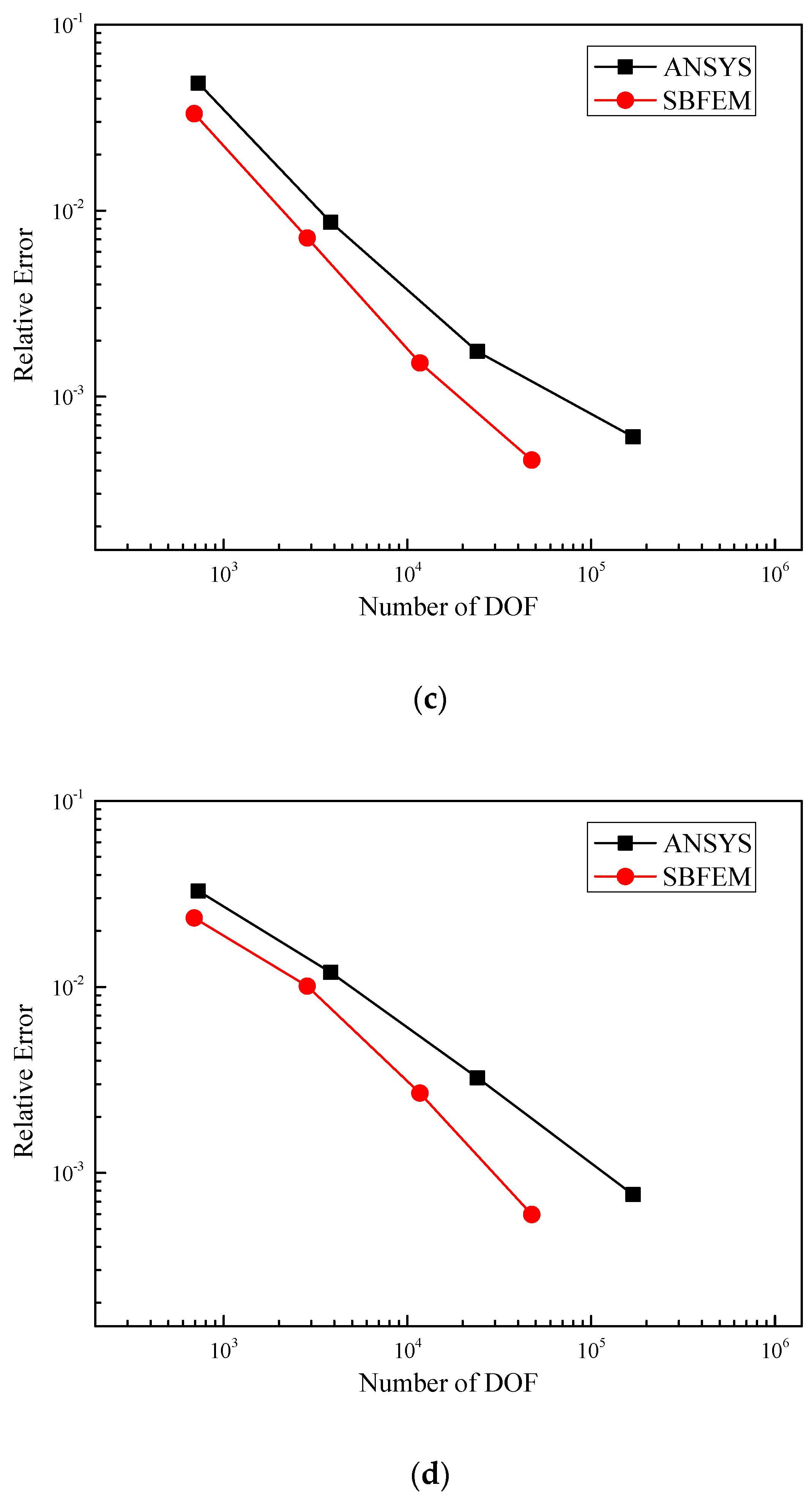
The relative error of displacements in the Z direction at endpoints C (0.0, 4.8, 1.0) and D (1.2, 4.8, 1.0) of the upper block are used to demonstrate the convergence of the SBFEM–BDEs. The results obtained by calculation model 5 in ANSYS are selected as the converged solution. As shown in Figure 5, the results of the SBFEM–BDEs and ANSYS converge to the same solution. When achieving results with the same precision, the SBFEM–BDEs consume DOF less than that of ANSYS.
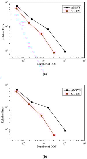
Figure 5.
The relative error of displacements in the Z direction vs. number of DOF. (a) The relative error of displacement in Z direction at endpoint C. (b) The relative error of in Z direction at endpoint D.
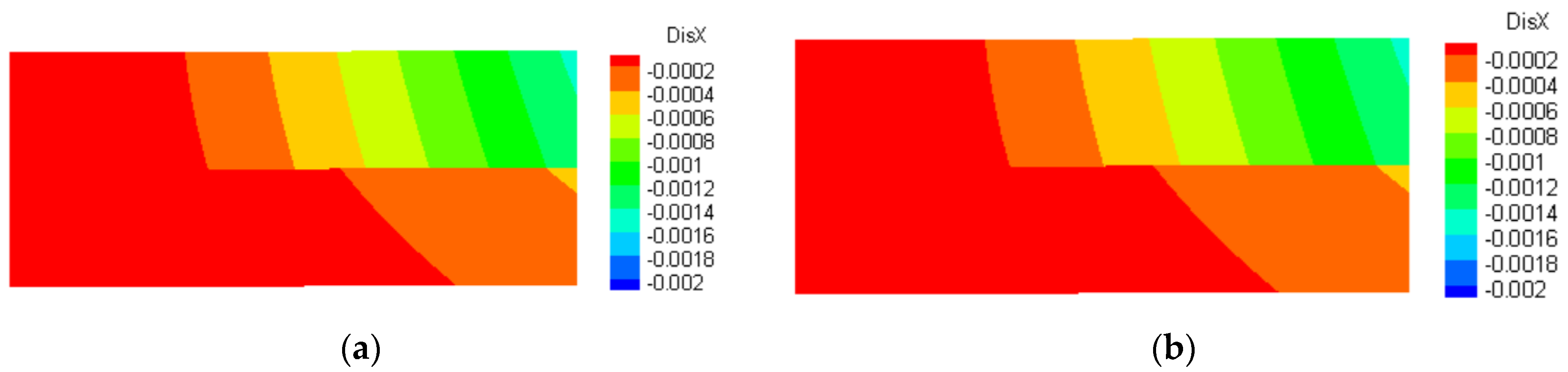
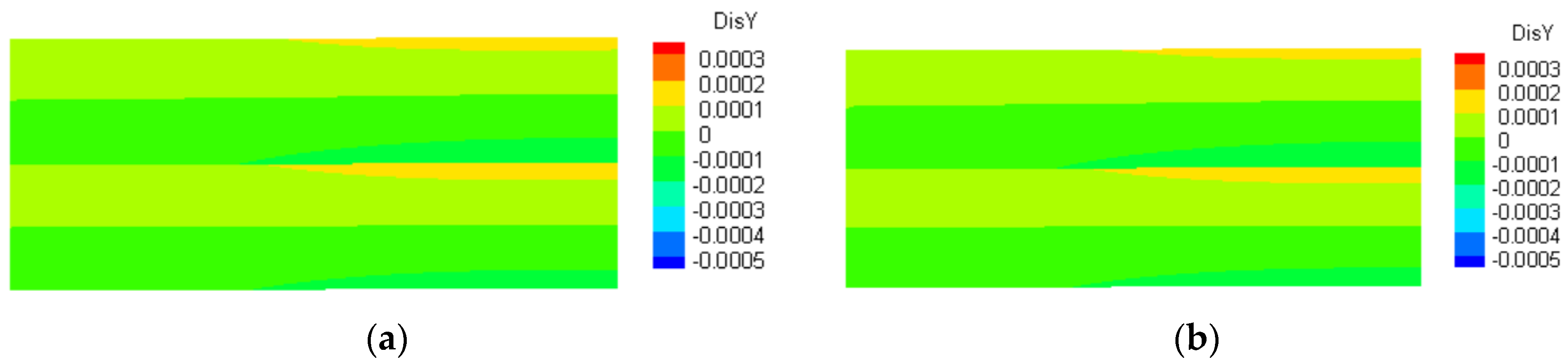
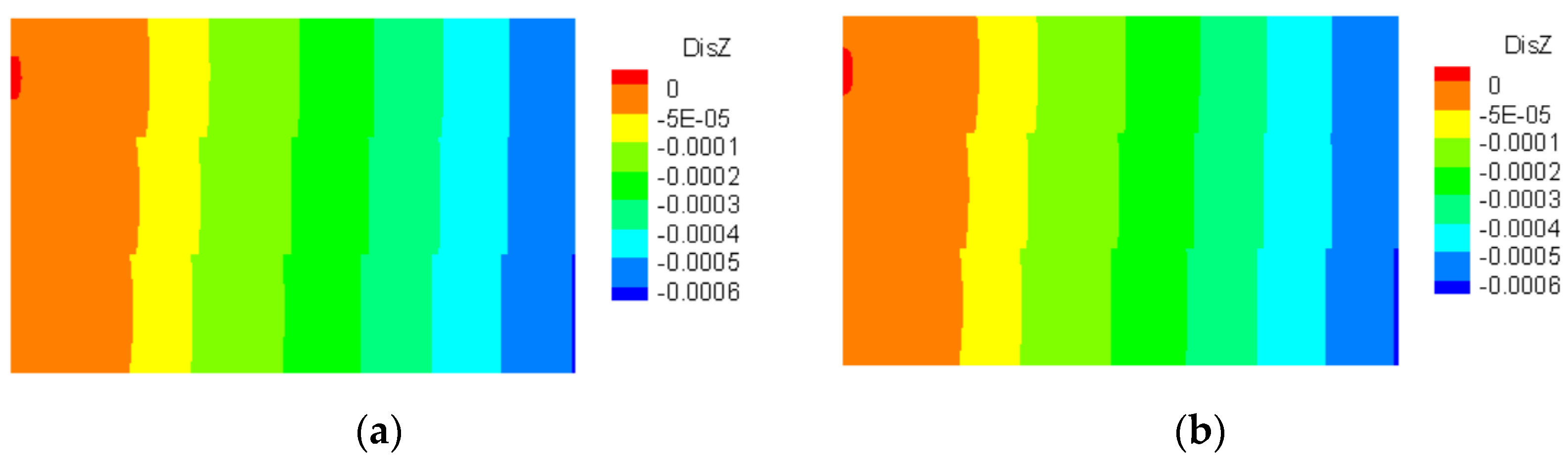
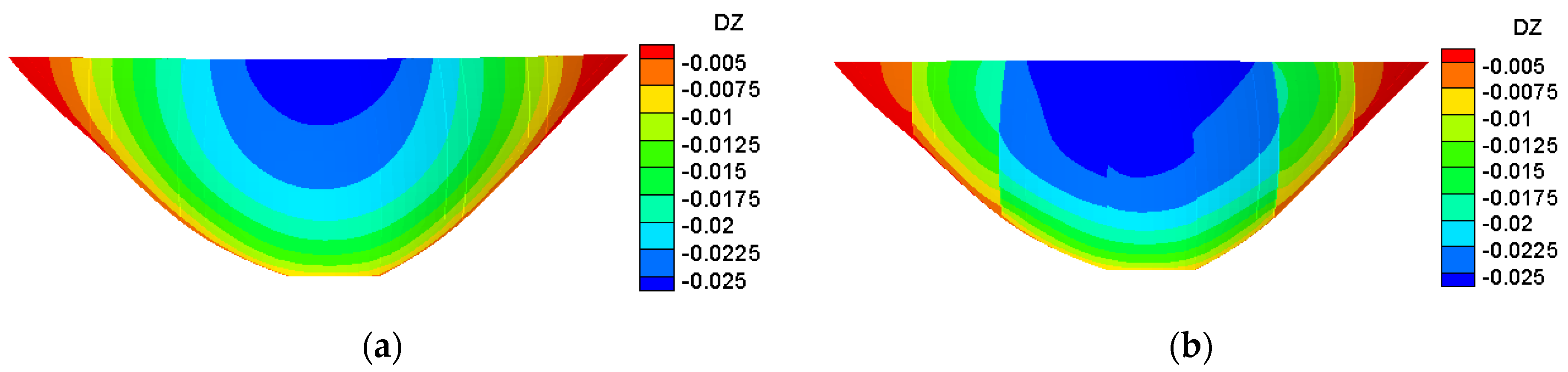
The displacement distributions in the slice from plane X = 0.6 m of calculation model 4 are shown in Figure 6, Figure 7 and Figure 8. As can be seen from Figure 6, Figure 7 and Figure 8, the displacement distributions calculated by the SBFEM–BDEs are in good agreement with those of ANSYS.

Figure 6.
The distribution of displacement in X-direction. (a) SBFEM. (b) ANSYS.
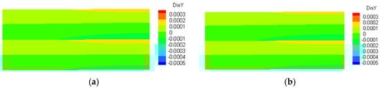
Figure 7.
The distribution of displacement in Y-direction. (a) SBFEM. (b) ANSYS.
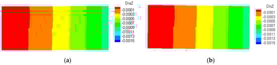
Figure 8.
The distribution of displacement in Z-direction. (a) SBFEM. (b) ANSYS.
5.2. Multiblock Contact Problem
In order to verify the accuracy of the proposed method in solving 3D frictional contact problems with multiple bodies, as shown in Figure 9, a three-block contact problem was selected for analysis. The size of each block is the same as that of the block in Section 5.1. The initial gap and frictional coefficient between the three blocks are 0 and 0.5, respectively. The elasticity modulus and Poisson’s ratio of the blocks are 30 GPa and 0.3, respectively. Concentrated forces of −100 kN are simultaneously applied along the X, Y and Z directions at endpoints of the top block. The left end of three blocks is fixed.
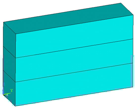
Figure 9.
Multibody contact.
In ANSYS, the frictional contact constraints are enforced by the augmented Lagrange multiplier method, and the mesh densities of different calculation models for each block are listed in Table 1. In the calculation model of the SBFEM, the mesh density of the surface element is equal to that of the solid element in the calculation model of ANSYS.
The relative error of displacements in the Z direction at endpoints A (0.0, 4.8, 2.0) and D (1.2, 4.8, 2.0) of the upper block, C (0.0, 4.8, 1.0) and D (1.2, 4.8, 1.0) of the middle block are used to demonstrate the convergence of the SBFEM–BDEs. The results obtained by calculation model 5 in ANSYS are selected as a converged solution. As shown in Figure 10, the results of the SBFEM–BDEs and ANSYS converge to the same solution. When achieving results with the same precision, the SBFEM–BDEs consume DOF less than that of ANSYS.
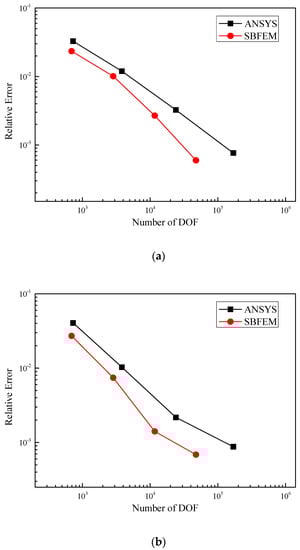
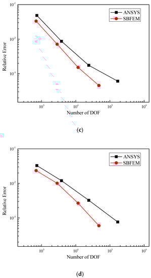
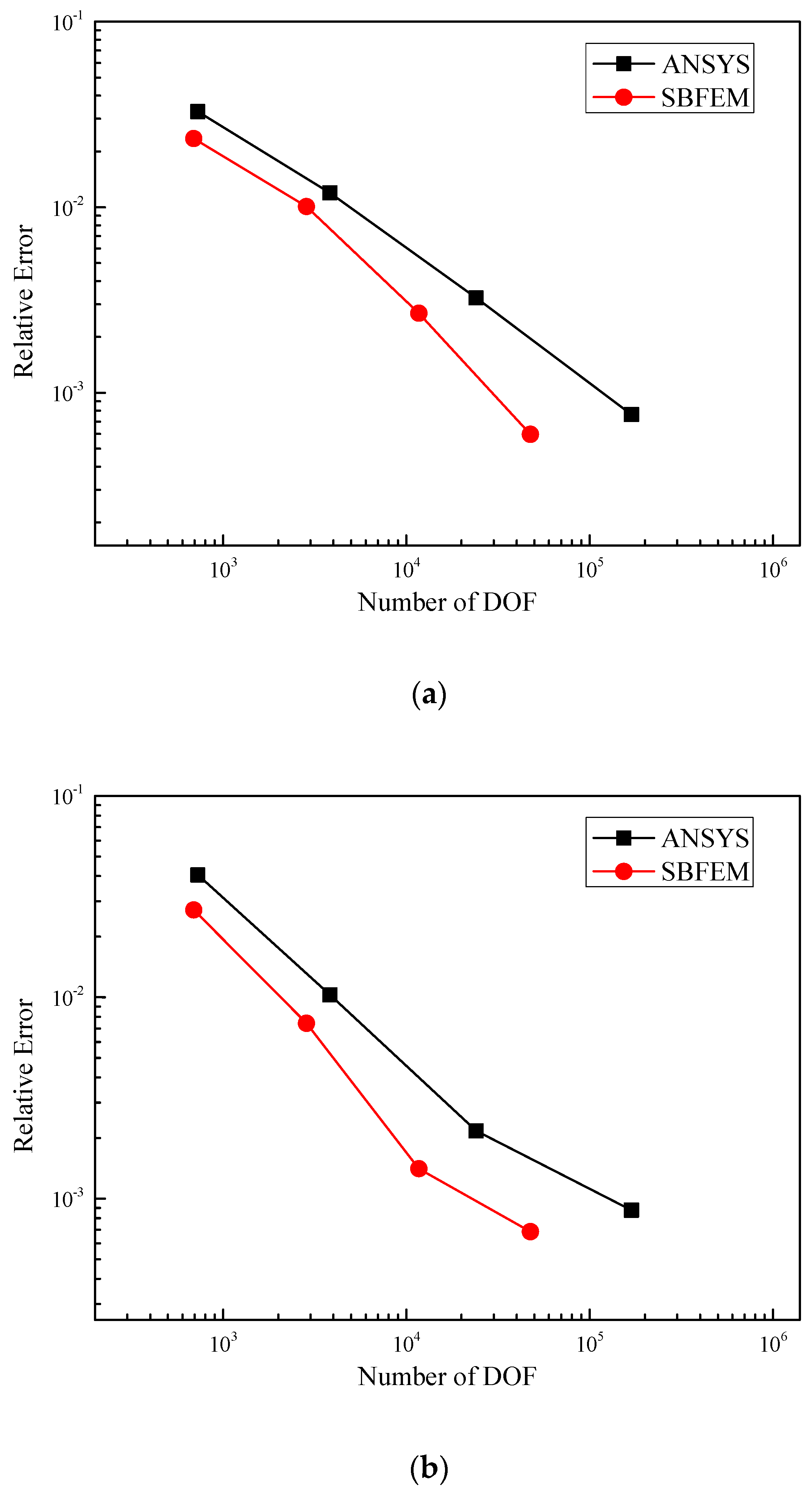
Figure 10.
The relative error of displacements in Z direction vs. number of DOF. (a) The relative error of displacement in Z direction at endpoint A. (b) The relative error of displacement in Z direction at endpoint B. (c) The relative error of displacement in Z direction at endpoint C. (d) The relative error of displacement in Z direction at endpoint D.
The displacement distributions in the slice from plane X = 0.6 m of the calculation model 4 are shown in Figure 11, Figure 12 and Figure 13. As can be seen from Figure 11, Figure 12 and Figure 13, the displacement distributions calculated by the SBFEM–BDEs are in good agreement with those of ANSYS.
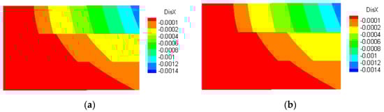
Figure 11.
The distribution of displacement in X-direction. (a) SBFEM. (b) ANSYS.
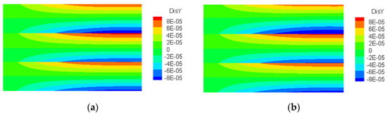
Figure 12.
The distribution of displacement in Y-direction. (a) SBFEM. (b) ANSYS.
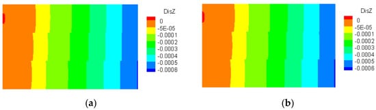
Figure 13.
The distribution of displacement in Z-direction. (a) SBFEM. (b) ANSYS.
5.3. Engineering Application
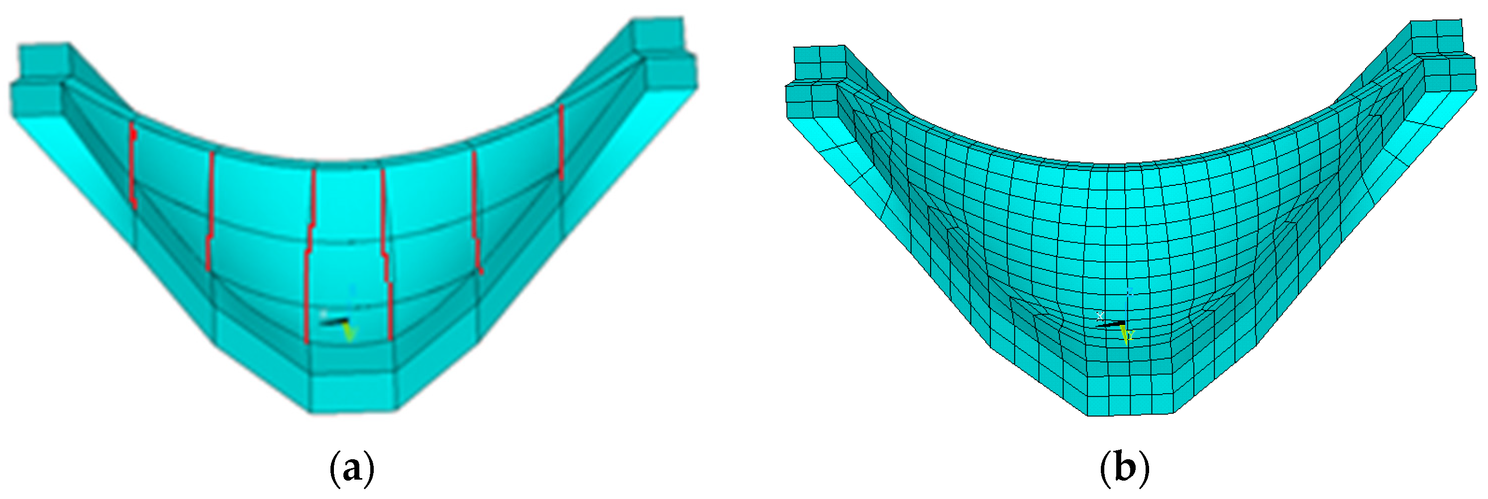
In order to verify the effectiveness of the SBFEM–BDEs to solve the arch-dam transverse joint contact problem, the arch-dam transverse joint calculation model, as shown in Figure 14, was selected for analysis. The location of the transverse joint is marked by a red line, as shown in Figure 14a. The elasticity modulus, Poisson’s ratio and mass density of the arch dam and near the foundation are 21 GPa, 0.167 and 2400 kg/m3, respectively. The height of the arch dam is 240 m. The dimensions of the near foundation are extended by a quarter of the dam height in the transverse direction, vertical direction and river direction, respectively. The effects of hydrostatic pressure and dam self-weight are considered in the analysis. The water level at the front of the dam is 240 m. The hydrostatic pressures are applied on the upstream surface of the dam. Fixed boundary conditions are applied on the bottom of the foundation. Two computing models were used for comparison. M1: The arch dam was considered as a monolithic block. M2: The transverse joints are assumed as a plane between each dam section. The frictional contact constraints of transverse joints are simulated by BDEs. The frictional coefficient of the transverse joint is set as 1.0. We assume that the water at the front of the dam cannot flow into the transverse joints. There are 1288 surface elements with 3612 nodes in M1 and M2.
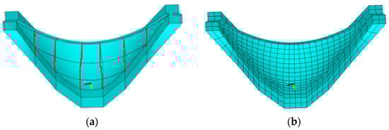
Figure 14.
The computing model of arch-dam contact problem. (a) Layout of transverse joints. (b) Surface elements.
The displacement distributions of the dam body in different directions are shown in Figure 15, Figure 16 and Figure 17. As can be seen from Figure 15, Figure 16 and Figure 17, the displacement obtained by M2 is bigger than that of M1. This is because the transverse joints weaken the overall stiffness of the dam body. In M2, the displacement continuity of the dam body in the transverse and downstream directions is low, which means the dam body slips along the transverse joints under the effects of hydrostatic pressure and gravity stress. The overall distribution trend of vertical displacement calculated by M2 is similar to that of M1, indicating that the existence of transverse joints has little influence on the vertical displacement of the dam body.
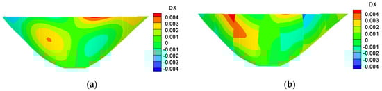
Figure 15.
The distribution of transverse displacement on the arch-dam upstream surface of different transverse joint models. (a) M1. (b) M2.
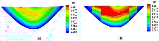
Figure 16.
The distribution of along-river displacement on the arch-dam upstream surface of different transverse joint models. (a) M1. (b) M2.
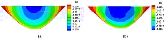
Figure 17.
The distribution of vertical displacement on the arch-dam upstream surface of different transverse joint models. (a) M1. (b) M2.
6. Conclusions
The scaled boundary finite-element method with B-differentiable equations is extended to 3D frictional contact problems. The two-block contact problem and the multiblock contact problem verify the effectiveness of the SBFEM–BDEs for 3D frictional contact problems. When achieving the same level of accuracy, the SBFEM–BDEs consume DOF less than those of ANSYS. This is because only the boundaries of the contact system are discretized into surface elements, and the dimension of the contact system is reduced by one when using the SBFEM. The arch-dam transverse joint contact problem shows that the proposed method can solve the practical engineering problem. The transverse joints weaken the overall stiffness of the dam body under the effects of hydrostatic pressure and gravity stress. The SBFEM–BDEs is a feasible and effective solution for frictional contact problems, and will be combined with fractal analysis to solve contact problems with rough surfaces in future work.
Author Contributions
Conceptualization, B.X. and X.D.; methodology, B.X.; software, B.X.; validation, X.D. and J.W.; formal analysis, X.Y.; investigation, X.D.; resources, J.W.; data curation, B.X.; writing—original draft preparation, B.X.; writing—review and editing, B.X.; visualization, X.D.; supervision, X.Y.; project administration, J.W.; funding acquisition, B.X. and X.D. All authors have read and agreed to the published version of the manuscript.
Funding
This research was funded by the National Natural Science Foundation of China (No. 52109169), the China Postdoctoral Science Foundation (No.2021M702951), the Natural Science Foundation of Henan (No. 212300410279), and the Open Fund of State Key Laboratory of Coastal and Offshore Engineering, Dalian University of Technology (No. LP2114).
Data Availability Statement
The data are available from the corresponding author upon request.
Conflicts of Interest
The authors declare no conflict of interest.
References
- Wriggers, P.; Scherf, O. Adaptive finite element techniques for frictional contact problems involving large elastic strains. Comput. Methods Appl. Mech. Eng. 1998, 151, 593–603. [Google Scholar] [CrossRef]
- Christensen, P.W.; Klarbring, A.; Pang, J.S.; Strömberg, N. Formulation and comparison of algorithms for frictional contact problems. Int. J. Numer. Methods Eng. 1998, 42, 145–173. [Google Scholar] [CrossRef]
- Hu, Z.Q.; Soh, A.K.; Chen, W.J.; Li, X.W.; Lin, G. Non-smooth Nonlinear Equations Methods for Solving 3D Elastoplastic Frictional Contact Problems. Comput. Mech. 2007, 39, 849–858. [Google Scholar] [CrossRef]
- Zhou, W.; Zhou, C.; Chang, X. A contact model based on the SQP algorithm and engineering application. Appl. Math. Comput. 2008, 198, 916–924. [Google Scholar]
- Lleras, V. A Stabilized Lagrange Multiplier Method for the Finite Element Approximation of Frictional Contact Problems in Elastostatics. Math. Model. Nat. Phenom. 2009, 4, 163–182. [Google Scholar] [CrossRef] [Green Version]
- Nguyen, V.T.; Hwu, C. Boundary element method for two-dimensional frictional contact problems of anisotropic elastic solids. Eng. Anal. Bound. Elem. 2019, 108, 49–59. [Google Scholar] [CrossRef]
- Vallepuga-Espinosa, J.; Sanchez-Gonzalez, L.; Ubero-Martinez, I. Winkler Support Model and Nonlinear Boundary Conditions Applied to 3D Elastic Contact Problem Using the Boundary Element Method. Acta Mech. Solida Sin. 2019, 32, 230–248. [Google Scholar] [CrossRef]
- Temizer, I.; Wriggers, P.; Hughes, T.J.R. Contact treatment in isogeometric analysis with NURBS. Comput. Methods Appl. Mech. Eng. 2011, 200, 1100–1112. [Google Scholar] [CrossRef]
- Temizer, I.; Wriggers, P.; Hughes, T.J.R. Three-dimensional mortar-based frictional contact treatment in isogeometric analysis with NURBS. Comput. Methods Appl. Mech. Eng. 2012, 209–212, 115–128. [Google Scholar] [CrossRef]
- De Lorenzis, L.; Wriggers, P.; Hughes, T.J.R. Isogeometric contact: A review. GAMM-Mitt. 2014, 37, 85–123. [Google Scholar] [CrossRef]
- Dimitri, R.; Zavarise, G. Isogeometric treatment of frictional contact and mixed mode debonding problems. Comput. Mech. 2017, 60, 315–332. [Google Scholar] [CrossRef]
- Wolf, J.P.; Song, C. The scaled boundary finite-element method-a primer: Derivations. Comput. Struct. 2000, 78, 191–210. [Google Scholar] [CrossRef]
- Song, C.; Wolf, J.P. The scaled boundary finite-element method-a primer: Solution procedures. Comput. Struct. 2000, 78, 211–225. [Google Scholar] [CrossRef]
- Yang, Z.J.; Wang, X.F.; Yin, D.S.; Zhang, C. A non-matching finite element-scaled boundary finite element coupled method for linear elastic crack propagation modelling. Comput. Struct. 2015, 153, 126–136. [Google Scholar] [CrossRef]
- Chen, D.; Dai, S. Dynamic fracture analysis of the soil-structure interaction system using the scaled boundary finite element method. Eng. Anal. Bound. Elem. 2017, 77, 26–35. [Google Scholar] [CrossRef]
- Li, J.; Gao, X.; Fu, X.-A.; Wu, C.; Lin, G. A Nonlinear Crack Model for Concrete Structure Based on an Extended Scaled Boundary Finite Element Method. Appl. Sci. 2018, 8, 1067. [Google Scholar] [CrossRef] [Green Version]
- Li, F.; Tu, Q. The Scaled Boundary Finite Element Analysis of Seepage Problems in Multi-Material Regions. Int. J. Comput. Methods 2012, 9, 1240008. [Google Scholar] [CrossRef]
- Bazyar, M.H.; Graili, A. A practical and efficient numerical scheme for the analysis of steady state unconfined seepage flows. Int. J. Numer. Anal. Methods Geomech. 2012, 36, 1793–1812. [Google Scholar] [CrossRef]
- Prempramote, S. A high-frequency open boundary for transient seepage analyses of semi-infinite layers by extending the scaled boundary finite element method. Int. J. Numer. Anal. Methods Geomech. 2016, 40, 919–941. [Google Scholar] [CrossRef]
- Wang, X.; Jin, F.; Prempramote, S.; Song, C. Time-domain analysis of gravity dam–reservoir interaction using high-order doubly asymptotic open boundary. Comput. Struct. 2011, 89, 668–680. [Google Scholar] [CrossRef]
- Lin, G.; Wang, Y.; Hu, Z. An efficient approach for frequency-domain and time-domain hydrodynamic analysis of dam-reservoir systems. Earthq. Eng. Struct. Dyn. 2012, 41, 1725–1749. [Google Scholar] [CrossRef]
- Lin, G.; Xue, B.; Hu, Z. A mortar contact formulation using scaled boundary isogeometric analysis. Sci. China Phys. Mech. Astron. 2018, 61, 074621. [Google Scholar] [CrossRef]
- Xing, W.; Song, C.; Tin-Loi, F. A scaled boundary finite element based node-to-node scheme for 2D frictional contact problems. Comput. Methods Appl. Mech. Eng. 2018, 333, 114–146. [Google Scholar] [CrossRef]
- Zhang, P.; Du, C.; Tian, X.; Jiang, S. A scaled boundary finite element method for modelling crack face contact problems. Comput. Methods Appl. Mech. Eng. 2018, 328, 431–451. [Google Scholar] [CrossRef]
- Zhang, P.; Du, C.; Birk, C.; Zhao, W. A scaled boundary finite element method for modelling wing crack propagation problems. Eng. Fract. Mech. 2019, 216, 106466. [Google Scholar] [CrossRef]
- Pramod, A.L.N.; Ooi, E.T.; Song, C.; Natarajan, S. An adaptive scaled boundary finite element method for contact analysis. Eur. J. Mech. A Solids 2021, 86, 104180. [Google Scholar]
- Zang, M.; Gao, W.; Lei, Z. A contact algorithm for 3D discrete and finite element contact problems based on penalty function method. Comput. Mech. 2011, 48, 541–550. [Google Scholar] [CrossRef]
- Antolin, P.; Buffa, A.; Fabre, M. A priori error for unilateral contact problems with Lagrange multipliers and isogeometric analysis. IMA J. Numer. Anal. 2019, 39, 1627–1651. [Google Scholar] [CrossRef] [Green Version]
- Stupkiewicz, S.; Lengiewicz, J.; Korelc, J. Sensitivity analysis for frictional contact problems in the augmented Lagrangian formulation. Comput. Methods Appl. Mech. Eng. 2010, 199, 2165–2176. [Google Scholar] [CrossRef]
- Ibán, A.L.; Garrido, J.A.; Prieto, I. Contact algorithm for non-linear elastic problems with large displacements and friction using the boundary element method. Comput. Methods Appl. Mech. Eng. 1999, 178, 51–67. [Google Scholar] [CrossRef]
- Wriggers, P. Computational Contact Mechanics; Springer: Berlin/Heidelberg, Germany, 2002. [Google Scholar]
- Alart, P.; Curnier, A. A mixed formulation for frictional contact problems prone to Newton like solution methods. Comput. Methods Appl. Mech. Eng. 1991, 92, 353–375. [Google Scholar] [CrossRef]
- Pang, J.S. Newton’s Method for B-Differentiable Equations. Math. Oper. Res. 1990, 15, 311–341. [Google Scholar] [CrossRef]


Publisher’s Note: MDPI stays neutral with regard to jurisdictional claims in published maps and institutional affiliations. |
© 2022 by the authors. Licensee MDPI, Basel, Switzerland. This article is an open access article distributed under the terms and conditions of the Creative Commons Attribution (CC BY) license (https://creativecommons.org/licenses/by/4.0/).