Fractional Behaviours Modelling with Volterra Equations: Application to a Lithium-Ion Cell and Comparison with a Fractional Model

Abstract

This paper proposes to model fractional behaviors using Volterra equations. As fractional differentiation-based models that are commonly used to model such behaviors exhibit several drawbacks and are particular cases of Volterra equations (in the kernel definition), it appears legitimate in a modeling approach to work directly with Volterra equations. In this paper, a numerical method is thus developed to identify the kernel associated to a Volterra equation that describes the input–output behavior of a system. This method is used to model a lithium-ion cell using real data. The resulting model is compared to a fractional differentiation-based model with the same number of tunable parameters.

1. Introduction

Fractional behaviors are induced by numerous physical phenomena, often of a stochastic nature, such as diffusion, collision, adsorption, freezing, aggregation, and fragmentation [1,2] Many examples of this type of behavior have been revealed in various areas, including electrochemistry [3,4], thermal science [5,6], biology [7,8], mechanics [9], acoustics [10], and electrical engineering [11]. Faced with the omnipresence of such behaviors, efficient modeling tools are required.

Physical systems with fractional behaviors are often modeled using fractional differentiation-based models, or “fractional models” for short. Such models are indeed able to fit the input–output behavior of this class of system accurately and with a limited number of parameters. However, it is now known that fractional differentiation-based models are associated to several drawbacks mainly related to the doubly infinite dimension of these models [12,13,14,15,16].

To overcome some of these drawbacks, new modeling tools must be introduced. Some were recently proposed in [12] among which Volterra equations are included. Volterra equations of the first kind were introduced by Volterra in [17] and, in the linear and homogenous case, are defined by the relation:

$${\int }_0^t\tilde{\eta }(t-\tau )x\left(\tau \right)\mathrm{d} \tau =v\left(t\right).$$

(1)

Assuming that $v\left(t\right)$ is differentiable, differentiation of the relation (1) leads to the following relation, which is called a linear Volterra equation of the second kind:

$$x\left(t\right)=u\left(t\right)+{\int }_0^t\eta (t-\tau )x\left(\tau \right)\mathrm{d} \tau ,$$

(2)

where $u\left(t\right)=\frac{1}{\tilde{\eta }\left(0\right)}\frac{\mathrm{d}}{\mathrm{d} t}v\left(t\right)$ and $\eta \left(t\right)=-\frac{1}{\tilde{\eta }\left(0\right)}\frac{\mathrm{d}}{\mathrm{d} t}\tilde{\eta }\left(t\right)$.

Volterra equations have been used in various applications: energy [18,19], sorption kinetics [20], and mechanical systems [21]. These equations are more general than the fractional differentiation-based models, since fractional pseudostate space descriptions are special cases of Volterra equations [22] involving a particular kernel. The Cole and Cole [23] modeling work considered by some as the first application of fractional differentiation could thus have been done using Volterra equations as demonstrated in [22].

This paper therefore proposes an answer to the problem of the direct determination of the kernel of a Volterra equation from input–output data. There is very little work in the literature that is interested in this problem, which is nevertheless an essential step in the modeling methodology. We can, however, cite the work of Brewer et al. [24], which relates to the identification of Volterra equation with weakly singular kernels but for which the kernel has a predefinite structure; and of Karuppiah et al. [25] which relates to the reconstruction of a time-independent parameter in an integrodifferential equation. We can also cite the work of Glentis et al. [26] in which Volterra kernels are estimated via statistics method, of Nemeth et al. [27] in which interpolating technics are used to approximate Volterra kernels, and of Lorenzi [28] in which some results on identification of unknown terms in integrodifferential equations are gathered. None of these works allow the direct computation of an analytic function for the kernel in the Volterra model to be obtained.

In this paper, it is first highlighted that Volterra equations generalize a pseudostate space description often used in the literature to model input–output fractional behaviors, but also other fractional models. An identification method that permits the direct determination of the kernel involved in a first-kind Volterra equation is then proposed. The method is applied to derive a model for a lithium-ion cell on real data. A comparison of the obtained model with a fractional differentiation based model is also carried out.

2. Volterra Equations as Generalizations of Fractional Models

For a fractional model, the pseudostate space descritpion is given by the relation

$$\left\{\begin{array}{cc}{D}_0^{\nu }x\hfill & =Ax\left(t\right)+Bu\left(t\right)\hfill \\ y\left(t\right)\hfill & =Cx\left(t\right)+Du\left(t\right)\hfill \end{array}\right.,\forall t<0,x\left(t\right)=u\left(t\right)=0,$$

(3)

where $D_0^{\nu }$ is a fractional differentiation operator of order $\nu \in \mathbb{R}$ [29], $x\left(t\right)\in {\mathbb{R}}^n$ is the pseudostate vector [30], $u\left(t\right)\in \mathbb{R}$ is the control input, supposed differentiable and $y\left(t\right)\in \mathbb{R}$ is the measured output. All these functions are supposed to be integrable over their domain of definition. Several definitions exist for this operator [31]. One of the most used definitions is that of Riemann–Liouville, denoted ${}_{RL}{D}_{t_0}^{\nu }$ with:

$${}_{RL}{D}_{t_0}^{\nu }f\left(t\right)=\frac{{\mathrm{d}}^m}{\mathrm{d} t^m}\left[\frac{1}{\mathsf{\Gamma }(m-\nu )}{\int }_{t_0}^t{(t-\tau )}^{m-\nu -1}f\left(\tau \right)\mathrm{d} \tau \right],$$

(4)

and $m=\lceil \nu \rceil$.

In the case $0<\nu <1$, a first order integration on both sides of the first equation of (3), leads to the following relation:

$${\int }_0^t\zeta (t-\tau )x\left(\tau \right)\mathrm{d} \tau ={\int }_0^{t}Ax\left(\tau \right)+Bu\left(\tau \right)\mathrm{d} \tau ,$$

(5)

where $\zeta (t-\tau )=\frac{{(t-\tau )}^{m-\nu -1}}{\mathsf{\Gamma }(m-\nu )}$ multiplies each component of the vector $x\left(\tau \right)$. The relation (5) can therefore be rewritten as follows

$${\int }_0^t\left(\zeta (t-\tau )I_n-A\right)x\left(\tau \right)\mathrm{d} \tau ={\int }_0^{t}Bu\left(\tau \right)\mathrm{d} \tau ,$$

(6)

where $I_n$ denotes the identity matrix of size n. And so the pseudo-state representation (3) can be rewritten as a Volterra equation of the first kind:

$${\int }_0^t\eta (t-\tau )x\left(\tau \right)\mathrm{d} \tau =v\left(t\right),$$

(7)

with $v\left(t\right)={\int }_0^{t}Bu\left(\tau \right)\mathrm{d} \tau$ and $\eta \left(t\right)=\zeta \left(t\right)I_n-A$. The relation (7) shows that the pseudostate representation is a particular case of Volterra equation of the first kind and thus of the second kind given relation (2).

This analysis can be extended to another class of fractional models. Consider the following fractional differential equation:

$$\sum _{k=1}^{N_a}{a}_k\frac{{\mathrm{d}}^{{\nu }_{a_k}}}{\mathrm{d} t^{{\nu }_{a_k}}}x\left(t\right)=\sum _{k=1}^{N_b}{b}_k\frac{{\mathrm{d}}^{{\nu }_{b_k}}}{\mathrm{d} t^{{\nu }_{b_k}}}u\left(t\right),$$

(8)

with

$$\begin{array}{cc}& {\nu }_{a_{N_a}}>{\nu }_{a_{N_a-1}}>\cdots >{\nu }_{a_1}\\ & {\nu }_{b_{N_b}}>{\nu }_{b_{N_b-1}}>\cdots >{\nu }_{b_1}\\ & {\nu }_{a_{N_a}}>{\nu }_{b_{N_b}}\mathrm{and}|{\nu }_{a_{N_a}}-{\nu }_{b_{N_b}}|<1.\end{array}$$

Laplace transform applied to relation (8) permits to write that

$$x\left(s\right)\frac{1}{F\left(s\right)}=u\left(s\right),$$

(9)

where $x\left(s\right)$ and $u\left(s\right)$ are respectively the Laplace transform of $x\left(t\right)$ and $u\left(t\right)$, and where

$$F\left(s\right)=\frac{{\sum }_{k=1}^{N_b}{b}_k{s}^{{\nu }_{b_k}}}{{\sum }_{k=1}^{N_a}{a}_k{s}^{{\nu }_{a_k}}}.$$

(10)

By multiplying the two sides of relation (9) by $\frac{1}{s}$, it becomes

$$x\left(s\right)\frac{1}{sF\left(s\right)}=\frac{1}{s}u\left(s\right),$$

(11)

in which transfer function $\frac{1}{sF\left(s\right)}$ is now proper.

Using the inverse Laplace transform, relation (11) becomes

$${\int }_0^t\phi (t-\tau )x\left(\tau \right)\mathrm{d} \tau =v\left(t\right),$$

(12)

with $v\left(t\right)={\int }_0^{t}u\left(\tau \right)\mathrm{d} \tau$ and where $\phi \left(t\right)={\mathcal{L}}^{-1}\left\{\frac{1}{sF\left(s\right)}\right\}$.

Relation (12) has thus the same form as relation (1) and is a first-kind Volterra equation with a kernel of specific structure.

Note that the constraint $|{\nu }_{a_{N_a}}-{\nu }_{b_{N_b}}|$ can be lifted. In the case $m-1<|{\nu }_{a_{N_a}}-{\nu }_{b_{N_b}}|<m$ ($m\in \mathbb{N}$), $v\left(t\right)$ is the integral of order m in relation (12) and $\phi \left(t\right)={\mathcal{L}}^{-1}\left\{\frac{1}{s^{m}F\left(s\right)}\right\}.$

As a consequence, in a modeling approach, it is better to work directly with a Volterra equation, because this avoids being constrained on the choice of the kernel, which is fixed in the case of a fractional model. The direct use of a Volterra equation is therefore more general.

3. A Numerical Method to Determine the Kernel of the Volterra Model

Let us denote $x\left(t\right)$ the output of a linear system in response to an input $u\left(t\right)$. The signal $x\left(t\right)$ is modeled with the Volterra equation of relation (2) which involves a kernel $\eta$ that can be determined numerically, as follows. A discretization of relation (2) is done using trapezoid method (with sampling time $T_s$), which provides:

$$\begin{array}{ccc}\hfill x\left(T_s\right)& =& u\left(T_s\right)+{\int }_0^{T_s}\eta \left(\tau \right)x(t-\tau )\mathrm{d} \tau \hfill \\ \hfill & \approx & u\left(T_s\right)+\frac{\eta \left(T_s\right)x(T_s-T_s)+\eta \left(0\right)x(T_s-0)}{2}{T}_s\hfill \\ \hfill x\left(2T_s\right)& =& u\left(2T_s\right)+{\int }_0^{T_s}\eta \left(\tau \right)x(t-\tau )\mathrm{d} \tau \hfill \\ & +& {\int }_{T_s}^{2T_s}\eta \left(\tau \right)x(t-\tau )\mathrm{d} \tau \hfill \\ \hfill & \approx & u\left(2T_s\right)+\frac{\eta \left(T_s\right)x(2T_s-T_s)+\eta \left(0\right)x(2T_s-0)}{2}{T}_s\hfill \\ & +& \frac{\eta \left(2T_s\right)x(2T_s-2T_s)+\eta \left(T_s\right)x(2T_s-T_s)}{2}{T}_s\hfill \\ & ⋮\end{array}$$

(13)

whose matrix writing is

$$\begin{array}{c}\hfill \underset{X}{\underbrace{\left[\begin{array}{cccccc}x\left(T_s\right)& x\left(0\right)& 0& \cdots & \cdots & \cdots \\ x\left(2T_s\right)& 2x\left(T_s\right)& x\left(0\right)& 0& \cdots & \cdots \\ x\left(3T_s\right)& 2x\left(2T_s\right)& 2x\left(T_s\right)& x\left(0\right)& 0& \cdots \\ & ⋮& \ddots \end{array}\right]}}\underset{\eta }{\underbrace{\left[\begin{array}{c}\eta \left(0\right)\\ \eta \left(T_s\right)\\ \eta \left(2T_s\right)\\ ⋮\end{array}\right]}}\\ \hfill =\underset{U}{\underbrace{\left[\begin{array}{c}x\left(T_s\right)-u\left(T_s\right)\\ x\left(2T_s\right)-u\left(2T_s\right)\\ x\left(3T_s\right)-u\left(3T_s\right)\\ ⋮\end{array}\right]}}\end{array}$$

(14)

Samples $\eta \left(k\right)$ can then be obtained solving the linear equation system (14) with a least square method. An analytic function $\eta \left(t\right)$ can then be used to fit the samples $\eta \left(k\right)$.

As an example, let suppose that the signal $x\left(t\right)$ corresponds to the step response of the fractional transfer function

$$F\left(s\right)=\frac{1}{{\left(\frac{s}{{\omega }_b}+1\right)}^{\nu }},\mathrm{with}{\omega }_b={10}^{-3}\mathrm{and}\nu =0.2.$$

(15)

The resulting step response is given by

$$\begin{array}{ccc}\hfill f\left(t\right)& =& \frac{{\mathrm{e}}^{-t/2{\omega }_b}{t}^{\nu }}{\nu (\nu +1)}\left({\left(\frac{t}{{\omega }_b}\right)}^{-\nu /2}{W}_M\left(\nu ,\nu /2+1/2,\frac{t}{{\omega }_b}\right)\right.\hfill \\ & +& \left.(\nu +1){\mathrm{e}}^{-t/2{\omega }_b}\right),\hfill \end{array}$$

(16)

where $W_M(·,·,·)$ is the Whittaker M function.

The samples $\eta \left(k\right)$ are then computed using relation (14). The following function, which is close to the impulse response of $F\left(s\right)$, is first considered to fit the samples $\eta \left(k\right)$ using relation (14):

$${\eta }_1\left(t\right)=a_0{t}^{\nu -1}exp(-t/{\omega }_b).$$

(17)

The response of Equation (2) with kernel ${\eta }_1\left(t\right)$ is denoted $x_1\left(t\right)$ and is compared to the response $x\left(t\right)$ of the fractional model (15) in Figure 1.

After optimization, the quadratic error between $x\left(t\right)$ and $x_1\left(t\right)$ is

$${\epsilon }_1=\sum {|x_1\left(i\right)-x\left(i\right)|}^2=5.5985.$$

(18)

Kernel (17) is singular. To avoid this singularity and to have a more accurate fitting of $\eta \left(k\right)$, another kernel must be found. For this, it is assumed that a physical system has a low-pass-type behavior, and thus its low-frequency behavior can be captured by a transfer function of the form

$$H\left(s\right)=\frac{1}{p^k(p+\alpha )},k\in \mathbb{N}.$$

(19)

Let $h\left(t\right)$ be the inverse Laplace transform of $H\left(s\right)$. To take into account the behavior of the system in medium frequency (frequencies less than $1/T_s$), function $h\left(t\right)$ is completed by a function of general form

$$g\left(t\right)=\frac{{\sum }_{k=1}^{n_a}{a}_k{t}^k}{{\sum }_{k=1}^{n_b}{b}_k{t}^k},\mathrm{with}{a}_0=1.$$

(20)

Thus for the considered problem (as $k=0$ in relation (19)), a possible analytic function for samples $\eta \left(k\right)$ fitting is:

$${\eta }_2\left(t\right)=exp(-\alpha t)\frac{1+a_{1}t+a_2{t}^2}{b_0+b_{1}t+b_2{t}^2}.$$

(21)

In Figure 2 are compared $\eta \left(k\right)$ and the kernel ${\eta }_2\left(t\right)$ with parameters gathered in

Table 1. Parameters of ${\eta }_2\left(t\right)$ in the relation (21).

$\mathit{\alpha }$	$4.2697\times {10}^{-5}$
$a_1$	$7.7946\times {10}^{-3}$
$a_2$	$2.3453\times {10}^{-5}$
$b_0$	$6.7661$
$b_1$	$4.2179$
$b_2$	$2.3728\times {10}^{-1}$

after optimization.

The quadratic error between ${\eta }_2\left(k\right)$ and $\eta \left(k{T}_s\right)$ is

$${\epsilon }_2=\sum {|{\eta }_2\left(i\right)-\eta \left(i\right)|}^2=3.6892\times {10}^{-3}.$$

(22)

The output of the model (2) with kernel ${\eta }_2\left(t\right)$, denoted $x_2\left(t\right)$ is given in Figure 3 and is compared with the response of the fractional model $f\left(t\right)$.

The quadratic error between $x_2\left(t\right)$ and $f\left(t\right)$ is

$${\epsilon }_3=\sum {|x_2\left(i\right)-x\left(i\right)|}^2=3.11\times {10}^{-1}.$$

(23)

The comparison reveals that the error ${\epsilon }_3$ obtained with the Volterra model is notably smaller than the error ${\epsilon }_1$ obtained with the fractional model. Thus, the proposed kernel of the general form

$$\eta \left(t\right)=h\left(t\right)g\left(t\right)$$

(24)

is a possible and interesting candidate for the fitting of the samples $\eta \left(k\right)$.

4. Application to Lithium-Ion Cell

This section is dedicated to lithium-ion cell input–output behavior modeling. A wide variety of battery models have been proposed in the literature with different complexities and applications. These models can be classified in 4 categories [32]

• Electrochemical models, which accurately describe electrochemical reactions that take place in the electrodes and the electrolyte [33]—Pseudo-Two-Dimensional model and Single Particle Model belong to this category;
• Mathematical models, which are based on empirical equations or math-based stochastic models which only evaluate the charge-recovery effect and ignore all other factors. The number of equations is reduced and simplified compared to the electrochemical model [34];
• Circuit-oriented models, which are electrical-equivalent models or impedance models in which each component of the circuit is related to an electrochemical process of the battery to provide a good description of its internal behaviour [35];
• Combined models that consists of the combination of different electrical models and mathematical models in order to combine the best attributes of each model, such as the correct prediction of the battery lifetime, steady-state and transient responses, and accurate estimation of the state of charge [36].

In this section, the model proposed falls in this last category as it is an impedance-based model, resulting from the simplification of Single Particle model, that combines several mathematical submodels, especially a Volterra equation, to take into the long-memory behaviour of a lithium-ion cell. This model will be compared to a similar model that includes a fractional order-transfer function [37].

The data comes from [38] and results from a collaboration with the society PSA Peugeot-Citroën. The input of the cell is the current and the output its voltage. The incoming current over time is plotted in Figure 4 and the resulting voltage $U\left(t\right)$ over time is plotted in Figure 5.

Under the asumption of material spherical particle in the electrodes and considering that the positive electrode is limiting in terms of dynamic behavior, a lithium-ion cell can be modeled by the single electrode model of Figure 6. This model contains a resistor R for the internal and connections resistances that can be estimated through the voltage drop that appears when a step current is applied. The function $\phi$ links the open circuit voltage (OCV) to the lithium concentration at the surface of the sphere. It can be obtained by measuring the cell voltage at rest for various cell states of charge. For the considered cell, this nonlinear function is fitted by a 12-degree polynomial (see [38] for the fitting result of this polynomial). The initial state of the battery is defined by $C_S\left(0\right)$ and the cell voltage is $U\left(t\right)$. The function $G\left(s\right)$ permits to model the diffusion of lithium inside the sphere.

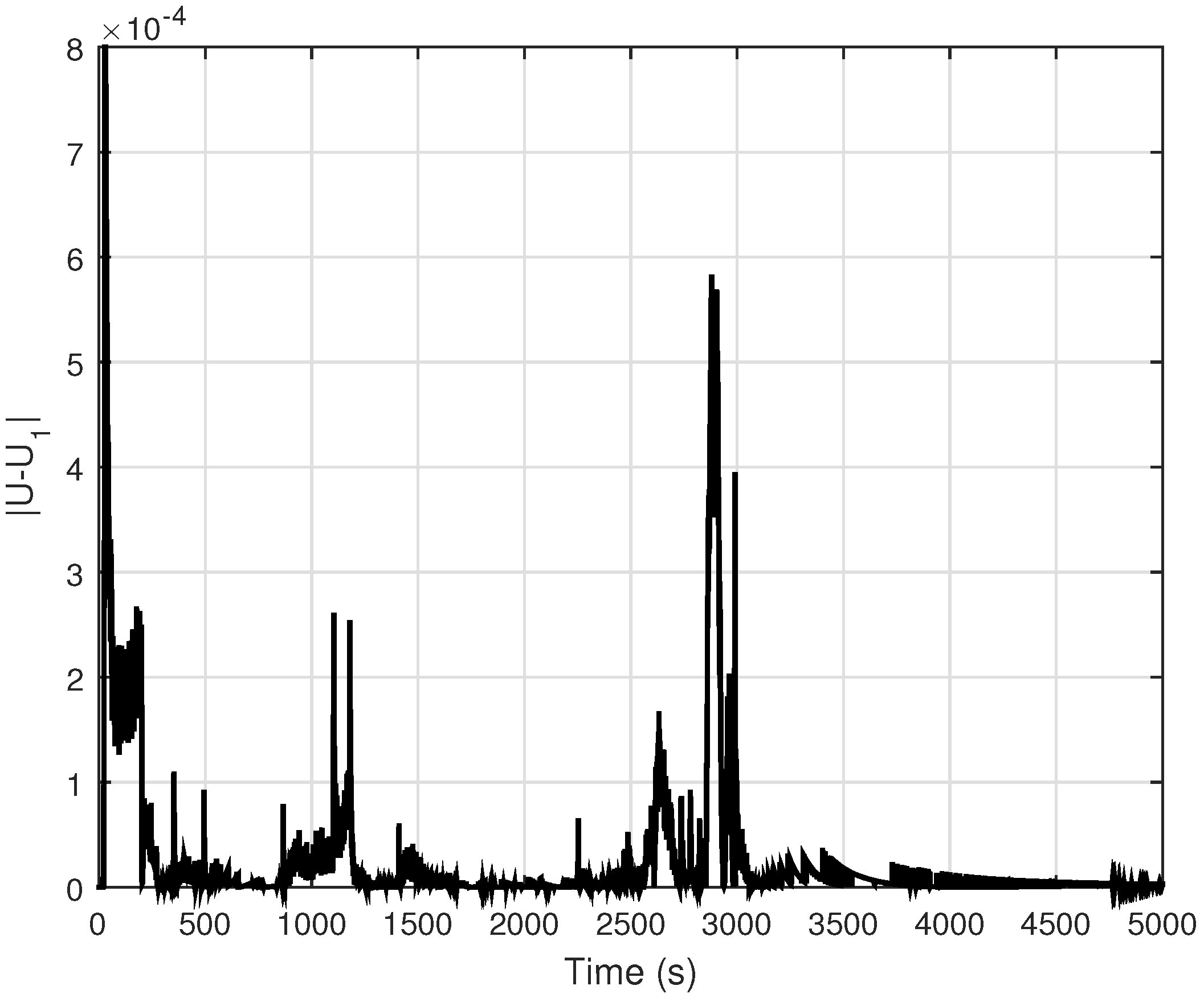
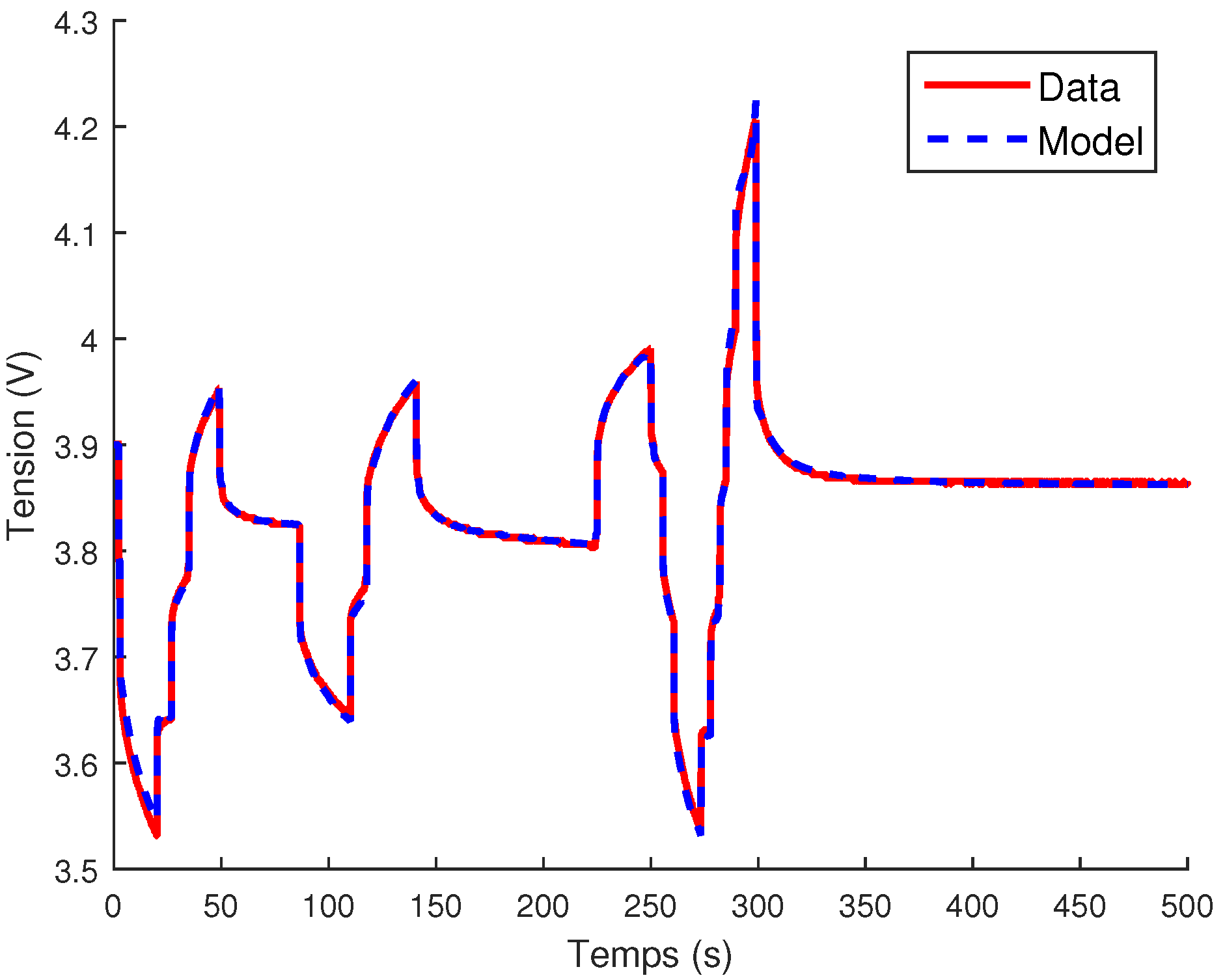
4.1. Fractional Model

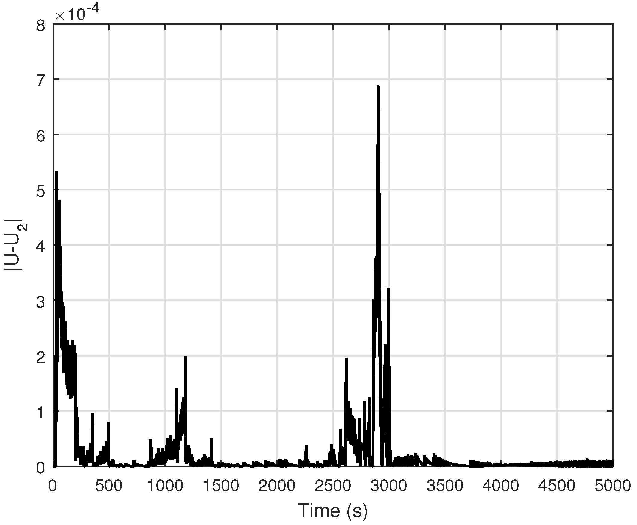
First, the diffusion part is modeled using the following fractional transfer function:

$$G\left(s\right)=\frac{K}{s}\frac{(1+\frac{s^n}{w_1})(1+\frac{s^n}{w_2})}{(1+\frac{s^n}{w_3})}.$$

(25)

After a least square optimization, aiming at minimizing the differences between the model and the cell output, the parameters gathered in

Table 2. Parameters of $G\left(s\right)$ from the relation (25) for modeling the outgoing battery voltage.

K	$4.332\times {10}^{-5}$
n	$7.195\times {10}^{-1}$
${\omega }_1$	$4.001\times {10}^{-2}$
${\omega }_2$	$1.143\times {10}^2$
${\omega }_3$	$4.345$

were obtained for transfer function $G\left(s\right)$. The optimal value for parameter R is $1.836\times {10}^{-3}$. The resulting response $U_1\left(t\right)$ of the model of Figure 6 is compared to the cell output voltage in Figure 7.

The quadratic error between $U\left(t\right)$ and $U_1\left(t\right)$ is given by:

$${\epsilon }_4=\sum {|U\left(i\right)-U_1\left(i\right)|}^2=1.250\times {10}^{-1}.$$

(26)

The error as a function of time is plotted in Figure 8.

4.2. Volterra Model

The diffusion part of the cell model described in Figure 6 is now modeled by the Volterra Equation (2), in which the kernel $\eta \left(t\right)$ is defined by the relation:

$${\eta }_2\left(t\right)=-exp(-\alpha t)\frac{1+a_0{t}^2}{b_0+a_1{t}^2+a_2{t}^3},$$

(27)

where function $u\left(t\right)$ is defined as $K_1\int I\left(t\right)$. Parameter $b_0=0.264$ is not optimized but is a fixed value defined so that the first value of $U_2\left(0\right)$ coincides with the voltage $U\left(0\right)$, where $U_2\left(t\right)$ denotes the Volterra equation-based cell model output. Hence, this model involves the same number of parameters as transfer function (25). After optimization, aiming at minimizing the differences between $U\left(t\right)$ and $U_2\left(t\right)$, the obtained parameters for ${\eta }_2\left(t\right)$ are gathered into

Table 3. Parameters of ${\eta }_2\left(t\right)$ of the relation (27) for the modeling of the outgoing battery voltage $U\left(t\right)$.

${\mathit{a}}_0$	$5.545\times {10}^{-1}$
$a_1$	$3.639\times {10}^{-2}$
$a_2$	$1.274\times {10}^{-3}$
$\alpha$	$3.965\times {10}^{-3}$
$K_1$	$4.486\times {10}^{-3}$

. The optimal value for parameter R is $1.836\times {10}^{-3}$.

The cell output voltage $U\left(t\right)$ and the output $U_2\left(t\right)$ of the model of Figure 6 using the Volterra model (2) for the diffusion part are compared in Figure 9.

The quadratic error between the voltage data $U\left(t\right)$ and the cell model is then given by

$${\epsilon }_5=\sum {|U\left(i\right)-U_2\left(i\right)|}^2=1.112\times {10}^{-1}.$$

(28)

The error as a function of time is plotted in Figure 10.

4.3. Discussion

In comparison with a simple first-order or second-order model, the Volterra model permits the system memory to be taken into account. The application of the previous section shows that both fractional and Volterra models accurately capture the dynamics of a system known for its fractional behaviour, with the same number of parameters and with a slightly better quadratic error for the Volterra model; however, one advantage of Volterra-based models is their ability to overcome several drawbacks of the fractional models [12,13,15]. Moreover, the Volterra model used here is simpler than single-particle models and pseudo-2D Li-ion electrochemical models.

Furthermore, the memory of a Volterra model can be limited by modifying one bound of the integral defining the Volterra model without affecting its input–output behavior. Relation (2) thus becomes:

$$x\left(t\right)=u\left(t\right)+{\int }_0^{T_f}\eta \left(\tau \right)x(t-\tau )\mathrm{d} \tau ,x\left(t\right)=0\mathrm{for}t<0$$

(29)

where $T_f$ characterizes the memory length.

By choosing $T_f$ well, the behaviors of (2) and (29) are very close. In order to define a rule for the choice of $T_f$, the frequency responses of the transfer function $x\left(s\right)/u\left(s\right)$ resulting from relation (29) for several values of $T_f$ are now compared.

As the Laplace transform of relation (29) is

$$x\left(s\right)=u\left(s\right)+{\int }_0^{T_f}\eta \left(\tau \right){\mathrm{e}}^{-s\tau }x\left(s\right)\mathrm{d} \tau$$

(30)

the transfer function $x\left(s\right)/u\left(s\right)$ is thus given by

$$\frac{x\left(s\right)}{u\left(s\right)}=\frac{1}{1-{\int }_0^{T_f}\eta \left(\tau \right){\mathrm{e}}^{-s\tau }\mathrm{d} \tau }.$$

(31)

For $s=j\omega$, integral in (31) can be computed numerically and thus, with $\Delta =\frac{T_f}{N}$:

$$\frac{x\left(j\omega \right)}{u\left(j\omega \right)}\approx \frac{1}{1-{\sum }_{k=0}^{N-1}\eta (k\Delta ){\mathrm{e}}^{-j\omega k\Delta }}.$$

(32)

Frequency responses of $x\left(j\omega \right)/u\left(j\omega \right)$ for $\eta \left(t\right)={\eta }_2\left(t\right)$ (relation (27)) and for $T_f=0.05/\alpha$, $T_f=0.1/\alpha ,T_f=1/\alpha ,T_f=5/\alpha$ and $T_f=10/\alpha$ are represented by Figure 11. This figure shows that for $T_f\ge 5/\alpha$ the Bode diagrams of $x\left(j\omega \right)/u\left(j\omega \right)$ are similar and that it is not useful to chose $T_f>5/\alpha$.

5. Conclusions

Starting from the idea that a fractional differentiation-based model is a particular type of Volterra equation [22], this paper proposes a method to directly derive an explicit form for the kernel involved in a Volterra equation from real input–output data. This method is based on the discretization of the Volterra equation and on the fitting of the discrete form of its kernel using an analytic function. The method is applied to the input–output modelling of a lithium-ion cell. The comparison of the resulting model response and the data reveals a very small error. This error is similar (but slightly better) to those obtained with a fractional differentiation-based models with the same number of tunable parameters but without the drawbacks associated to fractional differentiation-based models [12,13,14,15,16]. The authors now intend to continue working on fractional-behavior modeling using Volterra equations in order to improve the method presented in this paper (for instance, using a system of Volterra equations), and extend it in particular to multi-input multi-output systems. The authors also intend to work with other modelling tools, such as the one described in [39].

References

1. Krapivsky, P.L.; Redner, S.; Ben-Naim, E. A Kinetic View of Statistical Physics; Cambridge University Press: Cambridge, UK, 2010. [Google Scholar]
2. Family, F.; Landau, D. Kinetics of Aggregation and Gelation; Elsevier: Amsterdam, The Netherlands, 1984. [Google Scholar]
3. Rodrigues, S.; Munichandraiah, N.; Shukla, A. A review of state-of-charge indication of batteries by means of a.c. impedance measurements. J. Power Sources 2000, 87, 12–20. [Google Scholar] [CrossRef]
4. Sabatier, J.; Aoun, M.; Oustaloup, A.; Grégoire, G.; Ragot, F.; Roy, P. Fractional system identification for lead acid battery state of charge estimation. Signal Process. 2006, 86, 2645–2657. [Google Scholar] [CrossRef]
5. Battaglia, J.L.; Cois, O.; Puigsegur, L.; Oustaloup, A. Solving an inverse heat conduction problem using a non-integer identified model. Int. J. Heat Mass Transf. 2001, 44, 2671–2680. [Google Scholar] [CrossRef]
6. Malti, R.; Sabatier, J.; Akçay, H. Thermal modeling and identification of an aluminum rod using fractional calculus. IFAC Proc. Vol. 2009, 42, 958–963. [Google Scholar] [CrossRef] [Green Version]
7. Magin, R. Fractional Calculus in Bioengineering; Begell House Publishers Inc.: Danbury, CT, USA, 2006. [Google Scholar]
8. Ionescu, C.; De Keyser, R.; Sabatier, J.; Oustaloup, A.; Levron, F. Low frequency constant-phase behavior in the respiratory impedance. Biomed. Signal Process. Control 2011, 6, 197–208. [Google Scholar] [CrossRef]
9. Mainardi, F. Fractional Calculus and Waves in Linear Viscoelasticity; Imperial College Press: London, UK, 2010. [Google Scholar]
10. Matignon, D.; D’Andréa Novel, B.; Depalle, P.; Oustaloup, A. Viscothermal Losses in Wind Instruments: A Non Integer Model. In Proceedings of the International Symposium on the Mathematical Theory of Networks and Systems (MTNS), Regensburg, Germany, 2–6 August 1993. [Google Scholar]
11. Enacheanu, O. Modélisation fractale des réseaux électriques. Ph.D. Theses, Université Joseph-Fourier—Grenoble I, Grenoble, France, 2008. [Google Scholar]
12. Sabatier, J.; Farges, C.; Tartaglione, V. Some Alternative Solutions to Fractional Models for Modelling Power Law Type Long Memory Behaviours. Mathematics 2020, 8, 196. [Google Scholar] [CrossRef] [Green Version]
13. Dokoumetzidis, A.; Magin, R.; Macheras, P. A commentary on fractionalization of multi-compartmental models. J. Pharmacokinet. Pharmacodyn. 2010, 37, 203–207. [Google Scholar] [CrossRef] [PubMed]
14. Balint, A.M.; Balint, S. Mathematical Description of the Groundwater Flow and that of the Impurity Spread, which Use Temporal Caputo or Riemann–Liouville Fractional Partial Derivatives, Is Non-Objective. Fractal Fract. 2020, 4, 36. [Google Scholar] [CrossRef]
15. Sabatier, J. Fractional Order Models Are Doubly Infinite Dimensional Models and thus of Infinite Memory: Consequences on Initialization and Some Solutions. Symmetry 2021, 13, 1099. [Google Scholar] [CrossRef]
16. Sabatier, J.; Farges, C. Initial value problems should not be associated to fractional model descriptions whatever the derivative definition used. AIMS Math. 2021, 6, 11318. [Google Scholar] [CrossRef]
17. Volterra, V. Leçons sur les équations intégrales et les équations intégro-différentielles; Gauthier-Villars: Paris, France, 1913. [Google Scholar]
18. Markova, E.; Sidler, I.; Solodusha, S. Integral Models Based on Volterra Equations with Prehistory and Their Applications in Energy. Mathematics 2021, 9, 1127. [Google Scholar] [CrossRef]
19. Apartsin, A.; Sidler, I. Using the Nonclassical Volterra Equations of the First Kind to Model the Developing Systems. Autom. Remote Control 2013, 74, 899–910. [Google Scholar] [CrossRef]
20. Micke, A.; Bülow, M. Application of Volterra integral equations to the modelling of the sorption kinetics of multi-component mixtures in porous media: I. Fundamentals. Gas Sep. Purif. 1990, 4, 158–164. [Google Scholar] [CrossRef]
21. Szyłko-Bigus, O.; Śniady, P.; Zakęś, F. Application of Volterra integral equations in the dynamics of a multi-span Rayleigh beam subjected to a moving load. Mech. Syst. Signal Process. 2019, 121, 777–790. [Google Scholar] [CrossRef]
22. Sabatier, J. Fractional State Space Description: A Particular Case of the Volterra Equations. Fractal Fract. 2020, 4, 23. [Google Scholar] [CrossRef]
23. Cole, K.S.; Cole, R.H. Dispersion and Absorption in Dielectrics I. Alternating Current Characteristics. J. Chem. Phys. 1941, 9, 341–351. [Google Scholar] [CrossRef] [Green Version]
24. Brewer, D.; Powers, R. Parameter identification in a Volterra equation with weakly singular kernel. J. Integral Equ. Appl. 1990, 2, 353–373. [Google Scholar] [CrossRef]
25. Kannappan, K.; Kim, J.K.; Balachandran, K. Parameter Identification of an Integrodifferential Equation. Nonlinear Funct. Anal. Appl. 2015, 20, 169–185. [Google Scholar]
26. Glentis, G.O.; Koukoulas, P.; Kalouptsidis, N. Efficient algorithms for Volterra system identification. IEEE Trans. Signal Process. 1999, 47, 3042–3057. [Google Scholar] [CrossRef]
27. Nemeth, J.; Kollar, I.; Schoukens, J. Identification of Volterra kernels using interpolation. IEEE Trans. Instrum. Meas. 2002, 51, 770–775. [Google Scholar] [CrossRef]
28. Lorenzi, A. Identification problems for integrodifferential equations. In Ill-Posed Problems in Natural Sciences, Proceedings of the International Conference, Moscow, Russia, 19–25 August 1991; De Gruyter: Berlin, Germany, 2020; pp. 342–366. [Google Scholar] [CrossRef]
29. Samko, S.G.; Kilbas, A.A.; Marichev, O.I. Fractional Integrals and Derivatives: Theory and Applications; Gordon and Breach Science Publishers: New York, NY, USA, 1993. [Google Scholar]
30. Sabatier, J.; Farges, C.; Trigeassou, J.C. Fractional systems state space description: Some wrong ideas and proposed solutions. J. Vib. Control 2014, 20, 1076–1084. [Google Scholar] [CrossRef]
31. Tenreiro Machado, J. A Review of Definitions for Fractional Derivatives and Integral. Math. Probl. Eng. 2014, 2014, 238459. [Google Scholar] [CrossRef] [Green Version]
32. Tamilselvi, S.; Gunasundari, S.; Karuppiah, N.; Razak RK, A.; Madhusudan, S.; Nagarajan, V.M.; Sathish, T.; Shamim, M.Z.M.; Saleel, C.A.; Afzal, A. A Review on Battery Modelling Techniques. Sustainability 2021, 13, 42. [Google Scholar] [CrossRef]
33. Fuller, T.F.; Doyle, M.; Newman, J. Relaxation Phenomena in Lithium-Ion-Insertion Cells. J. Electrochem. Soc. 1994, 141, 982–990. [Google Scholar] [CrossRef] [Green Version]
34. Hu, T.; Zanchi, B.; Zhao, J. Simple Analytical Method for Determining Parameters of Discharging Batteries. IEEE Trans. Energy Convers. 2011, 26, 787–798. [Google Scholar] [CrossRef]
35. Saxena, S.; Raman, S.R.; Saritha, B.; John, V. A novel approach for electrical circuit modeling of Li-ion battery for predicting the steady-state and dynamic I–V characteristics. Sādhanā 2016, 41, 479–487. [Google Scholar] [CrossRef] [Green Version]
36. Chen, M.; Rincon-Mora, G. Accurate electrical battery model capable of predicting runtime and I-V performance. IEEE Trans. Energy Convers. 2006, 21, 504–511. [Google Scholar] [CrossRef]
37. Wang, Y.; Chen, Y.; Liao, X. State-of-art survey of fractional order modeling and estimation methods for lithium-ion batteries. Fract. Calc. Appl. Anal. 2019, 22, 1449–1479. [Google Scholar] [CrossRef]
38. Sabatier, J.; Francisco, J.M.; Guillemard, F.; Lavigne, L.; Moze, M.; Merveillaut, M. Lithium-ion batteries modeling: A simple fractional differentiation based model and its associated parameters estimation method. Signal Process. 2015, 107, 290–301. [Google Scholar] [CrossRef]
39. Sabatier, J. Modelling Fractional Behaviours Without Fractional Models. Front. Control Eng. 2021, 2, 716110. [Google Scholar] [CrossRef]
Figure 1. Fractional model (15) compared to the response x 1 ( t ) of model (2) with kernel η 1 ( t ) of Equation (17).
Fractalfract 06 00137 g001
Figure 2. Comparison of η ( k ) with η 2 ( t ) .
Fractalfract 06 00137 g002
Figure 3. Output x 2 ( t ) of model (2) with kernel η 2 ( t ) (Equation (21)) compared to the step response f ( t ) (Equation (16)).
Fractalfract 06 00137 g003
Figure 4. Input current applied to the cell.
Fractalfract 06 00137 g004
Figure 5. Cell output voltage.
Fractalfract 06 00137 g005
Figure 6. Model of a lithium-ion cell proposed in [38].
Fractalfract 06 00137 g006
Figure 7. Voltage U ( t ) compared to the response of model in Figure 6 with the fractional transfer function (25).
Fractalfract 06 00137 g007
Figure 8. Error between voltage U ( t ) and the response U 1 ( t ) of model in Figure 6 using the fractional transfer function (25).
Fractalfract 06 00137 g008
Figure 9. Voltage U ( t ) compared to the response U 2 ( t ) of model in Figure 6 using the Volterra model (2) with kernel (27).
Fractalfract 06 00137 g009
Figure 10. Error between voltage U ( t ) and the response U 2 ( t ) of model in Figure 6 using the Volterra model (2) with kernel (27).
Fractalfract 06 00137 g010
Figure 11. Frequency responses of x ( j ω ) / u ( j ω ) for η ( t ) = η 2 ( t ) , for various values of T f .
Fractalfract 06 00137 g011