The Mixed Boundary Value Problems and Chebyshev Collocation Method for Caputo-Type Fractional Ordinary Differential Equations

Abstract

The boundary value problem (BVP) for the varying coefficient linear Caputo-type fractional differential equation subject to the mixed boundary conditions on the interval $0\le x\le 1$ was considered. First, the BVP was converted into an equivalent differential–integral equation merging the boundary conditions. Then, the shifted Chebyshev polynomials and the collocation method were used to solve the differential–integral equation. Varying coefficients were also decomposed into the truncated shifted Chebyshev series such that calculations of integrals were only for polynomials and can be carried out exactly. Finally, numerical examples were examined and effectiveness of the proposed method was verified.

1. Introduction

In recent decades, the theory of fractional calculus has been attracting much attention partly due to its ability for describing memory and hereditary properties of various materials and processes [1,2,3,4,5,6,7]. Fractional calculus has been applied to different fields such as viscoelastic constitutive equations and related mechanical models [6,7,8,9,10,11], anomalous diffusion phenomena [4,6,12,13], hydrology [14], control and optimization theory [3,15], etc. It is worthwhile to mention that fractional calculus can be used to describe not only viscoelasticity, but also viscoinertia by different values of order [16,17]. The applications of fractional calculus lead to fractional differential equations (FDEs) in theory [2,3,4,5,18].

Let us recall some related definitions of fractional calculus used in this article. Let $f\left(x\right)$ be piecewise continuous on $(0,+\infty )$ and integrable on any finite subinterval of $(0,+\infty )$. Then, for $x>0$, the Riemann–Liouville fractional integral of $f\left(x\right)$ is defined as

$$I_x^{\beta }f\left(x\right)={\int }_0^x\frac{{(x-\tau )}^{\beta -1}}{\Gamma \left(\beta \right)}f\left(\tau \right)d\tau ,$$

(1)

for $\beta >0$, and $I_x^{0}f\left(x\right)=f\left(x\right)$ for $\beta =0$, where $\Gamma (·)$ is the gamma function. The fractional integral satisfies the following equalities:

$$\begin{array}{lll}& & I_x^{\beta }{I}_x^{\nu }f\left(x\right)=I_x^{\beta +\nu }f\left(x\right),\beta \ge 0,\nu \ge 0,\end{array}$$

(2)

$$\begin{array}{lll}& & I_x^{\nu }{x}^{\mu }=\frac{\Gamma (\mu +1)}{\Gamma (\mu +\nu +1)}{x}^{\mu +\nu },\nu \ge 0,\mu >-1.\end{array}$$

(3)

Let $\alpha$ be a positive real number, $m-1<\alpha \le m$, $m\in {\mathbb{N}}^{+}$, and $f^{\left(m\right)}\left(x\right)$ be piecewise continuous on $(0,+\infty )$ and integrable on any finite subinterval of $(0,+\infty )$. Then, the Caputo fractional derivative of $f\left(x\right)$ of order $\alpha$ is defined as

$$D_x^{\alpha }f\left(x\right)=I_x^{m-\alpha }{f}^{\left(m\right)}\left(x\right),m-1<\alpha \le m.$$

(4)

For the power function $x^{\mu }$, $\mu >0$, if $0\le m-1<\alpha \le m<\mu +1$, then we have

$$\begin{array}{rrr}{D}_x^{\alpha }{x}^{\mu }& =& \frac{\Gamma (\mu +1)}{\Gamma (\mu -\alpha +1)}{x}^{\mu -\alpha },x>0.\hfill \end{array}$$

(5)

The $\alpha$-order integral of the $\alpha$-order Caputo fractional derivative requires the knowledge of the initial values of the function and its integer-ordered derivatives,

$$I_x^{\alpha }{D}_x^{\alpha }f\left(x\right)=f\left(x\right)-\sum _{k=0}^{m-1}{f}^{\left(k\right)}\left(0\right)\frac{x^k}{k!},m-1<\alpha \le m.$$

(6)

This property enables the Caputo fractional derivative to be conveniently applied and analyzed.

In the earlier monograph [1], the Grünwald definition and the Riemann–Liouville definition of fractional calculus were introduced, where numerical differentiation and integration were considered and semi-integration was introduced by a designed electrical circuit model and semi-differentiation was applied to diffusion problems. The Weyl fractional calculus was introduced in [2] beside the Grünwald definition and the Riemann–Liouville definition. In [3], FDEs and fractional-order system and controllers were considered, where the Caputo fractional derivative was introduced. The existence, uniqueness and analytical methods of solutions for FDEs were investigated in [4]. In [18], the Caputo-type fractional derivative and FDEs were emphasized. In [6], fractional viscoelastic models and fractional wave models in viscoelastic media were introduced. In [5], numerical methods and fractional variational principle were reviewed.

Damping, deformation, vibration and dissipation arising from viscoelastic material can be modeled by FDEs [3,4,6,7]. The method of variable separation for fractional partial differential equation describing anomalous diffusion [4,6,12,14] can lead to a boundary value problem (BVP) for a fractional ordinary differential equation (ODE) [19]. The theorem of existence and uniqueness of solutions for fractional ODEs was presented in [3,4,18,20]. Some analytical and numerical methods were proposed to solve FDEs, e.g., see [3,4,5,21,22,23,24,25]. BVPs for fractional ODEs were considered in [19,26,27,28,29] by using the Adomian decomposition method, wavelet method, the method of upper and lower solutions, orthogonal polynomial method, etc. However, a fractional BVP with varying coefficients and mixed boundary conditions has hardly been considered.

In this work, we consider the BVP for the varying coefficient linear Caputo fractional ODE

$$\begin{array}{r}{D}_x^{\lambda }u\left(x\right)+c_1\left(x\right)u^{\prime }\left(x\right)+c_0\left(x\right)u\left(x\right)=g\left(x\right),0<x<1,1<\lambda \le 2,\end{array}$$

(7)

Subject to the mixed boundary conditions

$$\begin{array}{lll}& & p_{0}u\left(0\right)-q_0{u}^{\prime }\left(0\right)=b_0,\end{array}$$

(8)

$$\begin{array}{lll}& & p_{1}u\left(1\right)+q_1{u}^{\prime }\left(1\right)=b_1,\end{array}$$

(9)

where the coefficients $c_1\left(x\right)$, $c_0\left(x\right)$, $g\left(x\right)$ are specified continuous functions, the boundary parameters satisfy $p_0,q_0,p_1,q_1\ge 0$ and $p_0{p}_1+p_0{q}_1+q_0{p}_1\ne 0$. In the next Section 2, some preliminaries about the shifted Chebyshev polynomials are presented. In Section 3, we first convert the BVP, (7)–(9), into an equivalent fractional differential–integral equation merging the boundary conditions, then introduce the collocation method using the shifted Chebyshev polynomials of the first kind to solve the fractional differential–integral equation. Next, three numerical examples are solved by using the proposed method. Section 4 summarizes our conclusions.

2. The Shifted Chebyshev Polynomials of the First Kind

The Chebyshev polynomials of the first kind are defined by the formulae [30]

$$T_n\left(x\right)=\cos \left(n\arccos x\right),-1\le x\le 1,n=0,1,\dots .$$

(10)

They take on the explicit expressions as

$$T_0\left(x\right)=1,T_n\left(x\right)=\frac{n}{2}\sum _{k=0}^{[n/2]}{(-1)}^k\frac{(n-k-1)!}{k!(n-2k)!}{\left(2x\right)}^{n-2k},n\ge 1.$$

(11)

It is well-known that the Chebyshev polynomials of the first kind are orthogonal on the interval $[-1,1]$ with the weight function $\rho \left(x\right)=\frac{1}{\sqrt{1-x^2}},$ and $T_n\left(x\right)$ has exactly n zeros within the interval $(-1,1)$: ${\xi }_i=\cos \left(\frac{2i+1}{2n}\pi \right),$$i=0,1,\cdots ,n-1.$ The Chebyshev polynomials of the first kind satisfy the recurrence relation

$$T_0\left(x\right)=1,T_1\left(x\right)=x,T_n\left(x\right)=2x{T}_{n-1}\left(x\right)-T_{n-2}\left(x\right),n=2,3,\dots .$$

(12)

It is well-known that if $f\left(x\right)$ is $L_2$ integrable on $[-1,1]$ with the weight function $\rho \left(x\right)$, then its Chebyshev series expansion is $L_2$ convergent with respect to its weight function $\rho \left(x\right)$. If $f\left(x\right)$ has better smoothness, then stronger convergence can be attained for its Chebyshev series. If the function $f\left(x\right)$ has $n+1$ continuous derivatives on $[-1,1]$, then $|f\left(x\right)-S_{m}f\left(x\right)|=O\left(m^{-n}\right)$ for all $x\in [-1,1]$, where $S_{m}f\left(x\right)$ is the $(m+1)$-term truncation of the Chebyshev series expansion of $f\left(x\right)$. For more details for convergence, see [30].

In order to deal with the BVP on the interval $[0,1]$, we consider the shifted Chebyshev polynomials

$$T_n^{*}\left(x\right)=T_n(2x-1),x\in [0,1],n=0,1,\dots .$$

(13)

They are orthogonal on the interval $[0,1]$ with the weight function ${\rho }^{*}\left(x\right)=\frac{1}{\sqrt{x-x^2}},$ and the zeros of $T_n^{*}\left(x\right)$ are $x_i=\frac{1}{2}+\frac{1}{2}\cos \left(\frac{2i+1}{2n}\pi \right),$ $i=0,1,\dots ,n-1.$ As a complement to Equation (13), the shifted Chebyshev polynomials satisfy the relationship $T_n^{*}\left(x\right)=T_{2n}\left(\sqrt{x}\right).$ So, the explicit expressions of the shifted Chebyshev polynomials are conveniently obtained:

$$\begin{array}{r}{T}_0^{*}\left(x\right)=1,T_n^{*}\left(x\right)=n{\displaystyle \sum _{k=0}^n}{(-1)}^k\frac{(2n-k-1)!}{k!(2n-2k)!}{\left(4x\right)}^{n-k},n\ge 1.\end{array}$$

(14)

Finally, we mention the shifted Chebyshev polynomials of the second kind, which will also be used in the next section for the representation of solutions, $U_n^{*}\left(x\right)=U_n(2x-1),0\le x\le 1,n=0,1,\dots ,$ where $U_n\left(x\right)$ is the Chebyshev polynomials of the second kind.

3. The Equivalent Fractional Differential-Integral Equation and Chebyshev Collocation Method

First, we derive an equivalent differential–integral equation to the BVP (7)–(9). Applying the integral operator $I_x^{\lambda }(·)$ to both sides of Equation (7) and using Equation (6) yields

$$\begin{array}{r}u\left(x\right)-u\left(0\right)-u^{\prime }\left(0\right)x+I_x^{\lambda }(c_1\left(x\right)u^{\prime }\left(x\right)+c_0\left(x\right)u\left(x\right))=I_x^{\lambda }g\left(x\right).\end{array}$$

(15)

Our aim is to solve for $u\left(0\right)$ and $u^{\prime }\left(0\right)$ from the boundary conditions (8) and (9), and then obtain an equation about the solution $u\left(x\right)$ without any undetermined constants. Substituting $x=1$ in Equation (15) yields

$$\begin{array}{r}u\left(1\right)=u\left(0\right)+u^{\prime }\left(0\right)-I_{x,1}^{\lambda }(c_1\left(x\right)u^{\prime }\left(x\right)+c_0\left(x\right)u\left(x\right))+I_{x,1}^{\lambda }g\left(x\right),\end{array}$$

(16)

where the value of the fractional integral is defined for a general $\beta$th order integral of a function $v\left(x\right)$ at $x=\xi$ as

$$I_{x,\xi }^{\beta }v\left(x\right)={\int }_0^{\xi }\frac{{(\xi -\tau )}^{\beta -1}}{\Gamma \left(\beta \right)}v\left(\tau \right)d\tau .$$

(17)

Calculating the first order derivative on the both sides of Equation (15) leads to

$$\begin{array}{r}{u}^{\prime }\left(x\right)-u^{\prime }\left(0\right)+I_x^{\lambda -1}(c_1\left(x\right)u^{\prime }\left(x\right)+c_0\left(x\right)u\left(x\right))=I_x^{\lambda -1}g\left(x\right).\end{array}$$

(18)

Substituting $x=1$ yields

$$\begin{array}{r}{u}^{\prime }\left(1\right)=u^{\prime }\left(0\right)-I_{x,1}^{\lambda -1}(c_1\left(x\right)u^{\prime }\left(x\right)+c_0\left(x\right)u\left(x\right))+I_{x,1}^{\lambda -1}g\left(x\right).\end{array}$$

(19)

Substituting Equations (16) and (19) into Equation (9) yields

$$\begin{array}{r}{p}_{1}u\left(0\right)+(p_1+q_1)u^{\prime }\left(0\right)=b_1^{*},\end{array}$$

(20)

where

$$b_1^{*}=b_1+p_1{I}_{x,1}^{\lambda }(c_1\left(x\right)u^{\prime }\left(x\right)+c_0\left(x\right)u\left(x\right))-p_1{I}_{x,1}^{\lambda }g\left(x\right)+q_1{I}_{x,1}^{\lambda -1}(c_1\left(x\right)u^{\prime }\left(x\right)+c_0\left(x\right)u\left(x\right))-q_1{I}_{x,1}^{\lambda -1}g\left(x\right).$$

(21)

Equations (8) and (20) constitute a system of algebraic equations about $u\left(0\right)$ and $u^{\prime }\left(0\right)$. The coefficient determinant is

$$\begin{array}{r}P=p_0{p}_1+p_0{q}_1+q_0{p}_1,\end{array}$$

(22)

which is positive by our assumptions. Thus, we can solve the system of algebraic Equations (8) and (20) and obtain

$$\begin{array}{rrr}u\left(0\right)& =& \frac{(p_1+q_1)b_0}{P}+\frac{q_0{b}_1^{*}}{P},\hfill \end{array}$$

(23)

$$\begin{array}{rrr}{u}^{\prime }\left(0\right)& =& -\frac{p_1{b}_0}{P}+\frac{p_0{b}_1^{*}}{P}.\hfill \end{array}$$

(24)

Substituting Equations (23) and (24) into Equation (15), we obtain

$$\begin{array}{r}u\left(x\right)-\frac{(p_1+q_1)b_0}{P}+\frac{p_1{b}_0}{P}x-\frac{p_{0}x+q_0}{P}{b}_1^{*}+I_x^{\lambda }(c_1\left(x\right)u^{\prime }\left(x\right)+c_0\left(x\right)u\left(x\right))=I_x^{\lambda }g\left(x\right).\end{array}$$

(25)

Replacing $b_1^{*}$ by using Equation (21) and reorganizing the equation yield

$$\begin{array}{lll}& & u\left(x\right)-\frac{p_1(p_{0}x+q_0)}{P}{I}_{x,1}^{\lambda }(c_1\left(x\right)u^{\prime }\left(x\right)+c_0\left(x\right)u\left(x\right))\\ & & -\frac{q_1(p_{0}x+q_0)}{P}{I}_{x,1}^{\lambda -1}(c_1\left(x\right)u^{\prime }\left(x\right)+c_0\left(x\right)u\left(x\right))+I_x^{\lambda }(c_1\left(x\right)u^{\prime }\left(x\right)+c_0\left(x\right)u\left(x\right))=h\left(x\right),\hfill \end{array}$$

(26)

where

$$h\left(x\right)=\frac{(p_1+q_1)b_0-p_1{b}_{0}x}{P}+\frac{p_{0}x+q_0}{P}\left(b_1-p_1{I}_{x,1}^{\lambda }g\left(x\right)-q_1{I}_{x,1}^{\lambda -1}g\left(x\right)\right)+I_x^{\lambda }g\left(x\right),$$

(27)

Only involves the known boundary parameters and the known input function $g\left(x\right)$. Equation (26) is the equivalent differential–integral equation to the BVP (7)–((9). In the sequel, we seek for the solution to the differential-integral Equation (26).

We approximate the solution by an $(m+1)$-term truncation of the shifted Chebyshev series,

$${\phi }_m\left(x\right)=\sum _{n=0}^m{a}_n{T}_n^{*}\left(x\right),$$

(28)

where $a_n$, $n=0,1,\dots ,m$, are undetermined coefficients. Inserting ${\phi }_m\left(x\right)$ into Equation (26), we obtain the linear equation about $a_n$, $n=0,1,\dots ,m$,

$$\begin{array}{lll}& & {\displaystyle \sum _{n=0}^m}{a}_n\left(T_n^{*}\left(x\right)-\frac{p_1(p_{0}x+q_0)}{P}{I}_{x,1}^{\lambda }\left(c_1\left(x\right){T_n^{*}}^{\prime }\left(x\right)+c_0\left(x\right)T_n^{*}\left(x\right)\right)\right.\\ & & \left.-\frac{q_1(p_{0}x+q_0)}{P}{I}_{x,1}^{\lambda -1}\left(c_1\left(x\right){T_n^{*}}^{\prime }\left(x\right)+c_0\left(x\right)T_n^{*}\left(x\right)\right)+I_x^{\lambda }\left(c_1\left(x\right){T_n^{*}}^{\prime }\left(x\right)+c_0\left(x\right)T_n^{*}\left(x\right)\right)\right)=h\left(x\right).\hfill \end{array}$$

(29)

We note that in Equation (29), $I_{x,1}^{\lambda }\left(c_1\left(x\right){T_n^{*}}^{\prime }\left(x\right)+c_0\left(x\right)T_n^{*}\left(x\right)\right)$ and $I_{x,1}^{\lambda -1}$$\left(c_1\left(x\right){T_n^{*}}^{\prime }\left(x\right)+c_0\left(x\right)T_n^{*}\left(x\right)\right)$ are constants, represent the values of fractional integrals.

The collocation method may be applied to determine the coefficients $a_n$. The collocation points are taken as the zeroes of the $m+1$ degree shifted Chebyshev polynomial $T_{m+1}^{*}\left(x\right)$,

$$x_i=\frac{1}{2}+\frac{1}{2}\cos \left(\frac{2i+1}{2m+2}\pi \right),i=0,1,\dots ,m.$$

(30)

Thus, the collocation equation system is

$$\begin{array}{rrr}{\displaystyle \sum _{n=0}^m}{a}_n& & \left(T_n^{*}\left(x_i\right)-\frac{p_1(p_0{x}_i+q_0)}{P}{I}_{x,1}^{\lambda }\left(c_1\left(x\right){T_n^{*}}^{\prime }\left(x\right)+c_0\left(x\right)T_n^{*}\left(x\right)\right)\right.\hfill \\ & & -\frac{q_1(p_0{x}_i+q_0)}{P}{I}_{x,1}^{\lambda -1}\left(c_1\left(x\right){T_n^{*}}^{\prime }\left(x\right)+c_0\left(x\right)T_n^{*}\left(x\right)\right)\hfill \\ & & \left.+I_{x,x_i}^{\lambda }\left(c_1\left(x\right){T_n^{*}}^{\prime }\left(x\right)+c_0\left(x\right)T_n^{*}\left(x\right)\right)\right)=h\left(x_i\right),\hfill \end{array}$$

(31)

where

$$h\left(x_i\right)=\frac{(p_1+q_1)b_0-p_1{b}_0{x}_i}{P}+\frac{p_0{x}_i+q_0}{P}\left(b_1-p_1{I}_{x,1}^{\lambda }g\left(x\right)-q_1{I}_{x,1}^{\lambda -1}g\left(x\right)\right)+I_{x,x_i}^{\lambda }g\left(x\right),i=0,1,\dots ,m.$$

(32)

The matrix form of the collocation equation system (31) is

$$W\overrightarrow{a}=\overrightarrow{h},$$

(33)

where

$$\begin{array}{r}\overrightarrow{a}={(a_0,a_1,\dots ,a_m)}^T,\overrightarrow{h}={(h\left(x_0\right),h\left(x_1\right),\dots ,h\left(x_m\right))}^T,\end{array}$$

(34)

and the entries of the matrix W are

$$\begin{array}{rrr}{w}_{ij}& =& T_j^{*}\left(x_i\right)-\frac{p_1(p_0{x}_i+q_0)}{P}{I}_{x,1}^{\lambda }\left(c_1\left(x\right){T_j^{*}}^{\prime }\left(x\right)+c_0\left(x\right)T_j^{*}\left(x\right)\right)\hfill \\ & & -\frac{q_1(p_0{x}_i+q_0)}{P}{I}_{x,1}^{\lambda -1}\left(c_1\left(x\right){T_j^{*}}^{\prime }\left(x\right)+c_0\left(x\right)T_j^{*}\left(x\right)\right)+I_{x,x_i}^{\lambda }\left(c_1\left(x\right){T_j^{*}}^{\prime }\left(x\right)+c_0\left(x\right)T_j^{*}\left(x\right)\right),\hfill \\ & & i,j=0,1,\dots ,m.\hfill \end{array}$$

(35)

The solution of the linear algebraic equation system (31) or (33) gives the coefficients $a_n$ in Equation (28).

For the Dirichlet boundary conditions $u\left(0\right)=b_0,u\left(1\right)=b_1,$ the boundary parameters are simplified as $p_0=p_1=1$ and $q_0=q_1=0$, and thus Equation (31) degenerates to

$$\begin{array}{r}{\displaystyle \sum _{n=0}^m}{a}_n\left(T_n^{*}\left(x_i\right)-x_i{I}_{x,1}^{\lambda }\left(c_1\left(x\right){T_n^{*}}^{\prime }\left(x\right)+c_0\left(x\right)T_n^{*}\left(x\right)\right)+I_{x,x_i}^{\lambda }\left(c_1\left(x\right){T_n^{*}}^{\prime }\left(x\right)+c_0\left(x\right)T_n^{*}\left(x\right)\right)\right)=h\left(x_i\right),\end{array}$$

(36)

where $h\left(x_i\right)=b_0+(b_1-b_0)x_i-x_i{I}_{x,1}^{\lambda }g\left(x\right)+I_{x,x_i}^{\lambda }g\left(x\right),i=0,1,\dots ,m.$

We remark that by the relationship of the first-kind and second-kind Chebyshev polynomials ${T_n}^{\prime }\left(x\right)=n{U}_{n-1}\left(x\right)$, we have the relationship of the shifted Chebyshev polynomials of the two kinds

$${T_n^{*}}^{\prime }\left(x\right)=2n{U}_{n-1}^{*}\left(x\right).$$

(37)

So, the derivative ${T_n^{*}}^{\prime }\left(x\right)$ in Equations (31), (35) and (36) may be replaced by the second-kind Chebyshev polynomials.

The operators $I_{x,1}^{\lambda }(·)$, $I_{x,1}^{\lambda -1}(·)$ and $I_{x,x_i}^{\lambda }(·)$ in Equations (31), (32) and (35) represent the values of fractional integrals of the known functions. Since the appearance of the varying coefficients $g\left(x\right)$ and $c_k\left(x\right)$, manual computations for these integrals are laborious in general. Here we approximate the varying coefficients again using their truncated shifted Chebyshev series as

$$\begin{array}{r}g\left(x\right)={\displaystyle \underset{n=0}{\overset{M}{{\sum }^{\prime }}}}{g}_n{T}_n^{*}\left(x\right),c_k\left(x\right)={\displaystyle \underset{n=0}{\overset{M}{{\sum }^{\prime }}}}{c}_{k,n}{T}_n^{*}\left(x\right),k=0,1,0\le x\le 1,\end{array}$$

(38)

where

$$\begin{array}{rrr}{g}_n& =& \frac{2}{\pi }{\int }_0^1\frac{1}{\sqrt{x-x^2}}g\left(x\right)T_n^{*}\left(x\right)dx,n=0,1,\dots ,M,\hfill \end{array}$$

(39)

$$\begin{array}{rrr}{c}_{k,n}& =& \frac{2}{\pi }{\int }_0^1\frac{1}{\sqrt{x-x^2}}{c}_k\left(x\right)T_n^{*}\left(x\right)dx,k=0,1,n=0,1,\dots ,M,\hfill \end{array}$$

(40)

and the superscript ${}^{\prime }$ of ∑ denotes that the first term in the sum is halved. We note that there is no need of connections between the values of m and M in Equations (28) and (38). Utilizing the Gauss–Chebyshev quadrature formula we derive the numerical formulae for $g_n$ and $c_{k,n}$ as

$$\begin{array}{rrr}{g}_n& =& \frac{2}{M+1}{\displaystyle \sum _{i=0}^M}g\left(x_i\right)T_n^{*}\left(x_i\right),n=0,1,\dots ,M,\hfill \end{array}$$

(41)

$$\begin{array}{rrr}{c}_{k,n}& =& \frac{2}{M+1}{\displaystyle \sum _{i=0}^M}{c}_k\left(x_i\right)T_n^{*}\left(x_i\right),k=0,1,n=0,1,\dots ,M,\hfill \end{array}$$

(42)

where $x_i$ are the zeroes of the $M+1$ degree shifted Chebyshev polynomial $T_{M+1}^{*}\left(x\right)$,

$$x_i=\frac{1}{2}+\frac{1}{2}\cos \left(\frac{2i+1}{2M+2}\pi \right),i=0,1,\dots ,M.$$

(43)

Thus, making use of the decompositions in (38), the calculation of the integrals $I_{x,1}^{\lambda }(·)$, $I_{x,1}^{\lambda -1}(·)$ and $I_{x,x_i}^{\lambda }(·)$ in Equations (31), (32) and (35) only involves integrals of polynomials, so can be carried out exactly.

In the following three examples, we take $M=5$ in Equation (38) to truncate the decompositions of the coefficients $g\left(x\right)$ and $c_k\left(x\right)$ and to calculate the involved integrals $I_{x,1}^{\lambda }(·)$, $I_{x,1}^{\lambda -1}(·)$ and $I_{x,x_i}^{\lambda }(·)$. Collocation equation systems are solved by using Mathematica command “LinearSolve”. Figures of approximate analytical solutions and errors are generated by using Mathematica.

Example 1.

Consider the BVP for the linear FDE

$$\begin{array}{lll}& & D_x^{1.5}u\left(x\right)-\frac{x\sin \left(x\right)}{3}{u}^{\prime }\left(x\right)+\sin \left(x\right)u\left(x\right)=g\left(x\right),0<x<1,\end{array}$$

(44)

$$\begin{array}{lll}& & u^{\prime }\left(0\right)=-1,u\left(1\right)=1,\end{array}$$

(45)

where$g\left(x\right)=\frac{3\sqrt{\pi }}{4}+\frac{8x^{1.5}}{\sqrt{\pi }}-\frac{2}{3}x\sin \left(x\right)+\frac{1}{2}{x}^{1.5}\sin \left(x\right).$

The BVP has the exact solution $u^{*}\left(x\right)=-x+x^{1.5}+x^3.$ The boundary parameters are $p_0=0,q_0=-1,b_0=-1$, $p_1=1,q_1=0,b_1=1.$ The collocation equation system in (31) is

$$\begin{array}{rrr}{\displaystyle \sum _{n=0}^m}{a}_n& & \left(T_n^{*}\left(x_i\right)-I_{x,1}^{1.5}\left(\frac{-x\sin \left(x\right)}{3}{T_n^{*}}^{\prime }\left(x\right)+\sin \left(x\right)T_n^{*}\left(x\right)\right)\right.\hfill \\ & & \left.+I_{x,x_i}^{1.5}\left(\frac{-x\sin \left(x\right)}{3}{T_n^{*}}^{\prime }\left(x\right)+\sin \left(x\right)T_n^{*}\left(x\right)\right)\right)=h\left(x_i\right),\hfill \end{array}$$

(46)

where $h\left(x_i\right)=2-x_i-I_{x,1}^{1.5}g\left(x\right)+I_{x,x_i}^{1.5}g\left(x\right),i=0,1,\dots ,m.$

Take $m=2,3,4$ and 5, respectively, the solution approximations ${\phi }_m\left(x\right)$ are calculated as

$$\begin{array}{rrr}{\phi }_2\left(x\right)& =& 0.0175774-1.10039x+2.05832x^2,\hfill \\ \hfill {\phi }_3\left(x\right)& =& -0.00586106-0.689478x+0.925577x^2+0.768798x^3,\hfill \\ \hfill {\phi }_4\left(x\right)& =& -0.00288415-0.76024x+1.24242x^2+0.293418x^3+0.22758x^4,\hfill \\ \hfill {\phi }_5\left(x\right)& =& -0.00167028-0.8038x+1.54387x^2-0.47843x^3+1.05648x^4-0.316564x^5.\hfill \end{array}$$

The error function and maximum error of the approximate solution ${\phi }_m\left(x\right)$ are defined as

$$E{R}_m\left(x\right)=\left|{\phi }_m\left(x\right)-u^{*}\left(x\right)\right|\mathrm{and}M{E}_m=\underset{0\le x\le 1}{\max }E{R}_m\left(x\right).$$

(47)

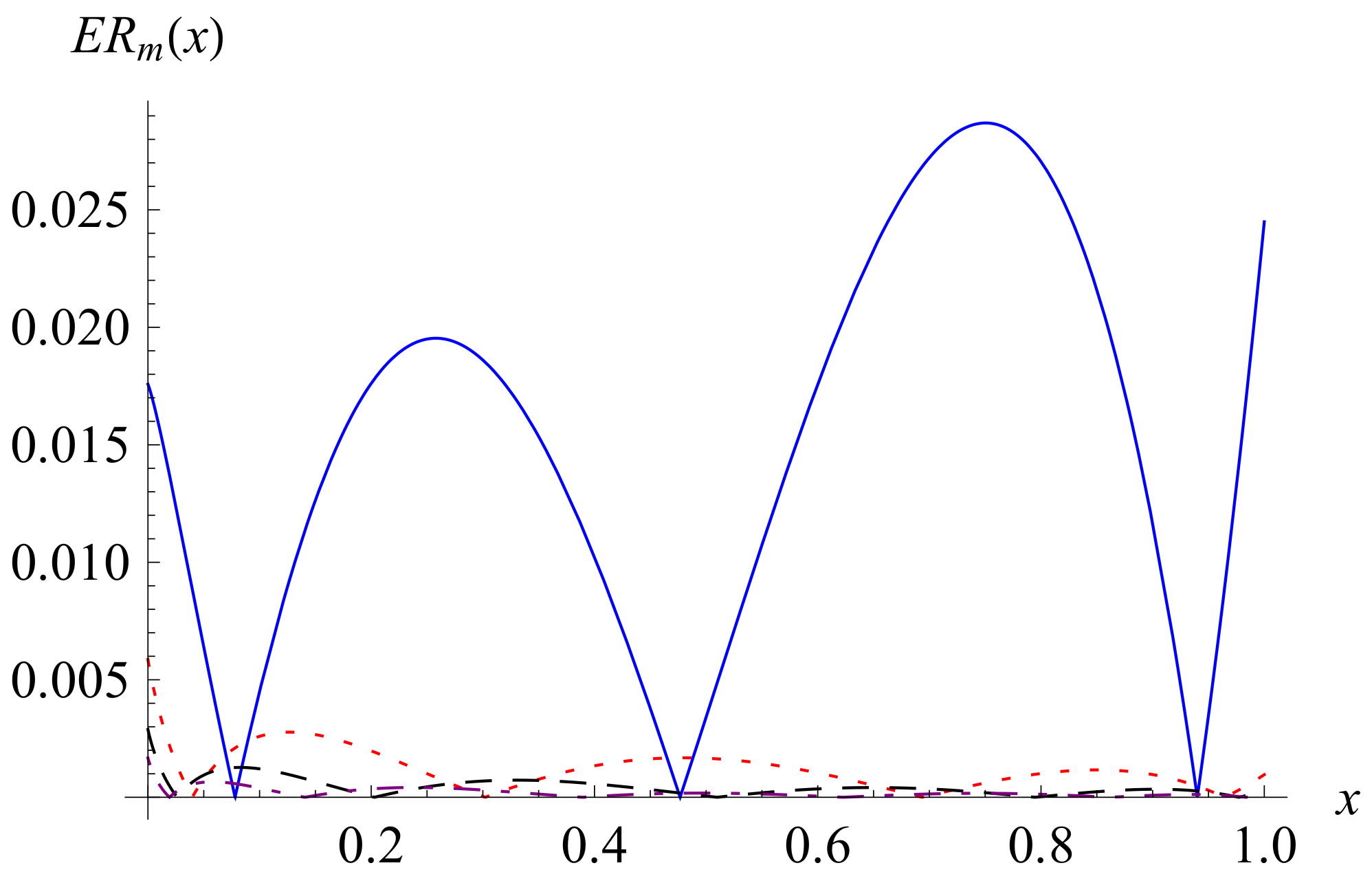
In Figure 1, the error functions $E{R}_m\left(x\right)$ for $m=2,3,4,5$ are depicted, where at the $m+1$ collocation points of ${\phi }_m\left(x\right)$, errors are zero. The maximum errors of the four approximate solutions are 0.028696, 0.005861, 0.002884, and 0.001670, respectively.

Figure 1. The error functions $E{R}_m\left(x\right)$ for $m=2$ (solid line), $m=3$ (dot line), $m=4$ (dash line) and $m=5$ (dot-dash line).

Example 2.

Consider the BVP for the linear FDE

$$\begin{array}{lll}& & D_x^{\lambda }u\left(x\right)-u\left(x\right)=-4x{e}^x,0<x<1,1<\lambda \le 2,\end{array}$$

(48)

$$\begin{array}{lll}& & u\left(0\right)-u^{\prime }\left(0\right)=-1,u\left(1\right)+u^{\prime }\left(1\right)=-e.\end{array}$$

(49)

If $\lambda =2$, the BVP has the exact solution $u^{*}\left(x\right)=x(1-x)e^x.$

For this example, the coefficients and parameters are $c_1\left(x\right)=0$, $c_0\left(x\right)=-1$, $g\left(x\right)=-4x{e}^x,$ $p_0=q_0=p_1=q_1=1$, $b_0=-1$ and $b_1=-e.$ The collocation equation system in Equation (31) becomes

$$\begin{array}{lll}& & {\displaystyle \sum _{n=0}^m}{a}_n\left(T_n^{*}\left(x_i\right)-\frac{x_i+1}{3}{I}_{x,1}^{\lambda }\left(-T_n^{*}\left(x\right)\right)\right.\\ & & -\left.\frac{x_i+1}{3}{I}_{x,1}^{\lambda -1}\left(-T_n^{*}\left(x\right)\right)+I_{x,x_i}^{\lambda }\left(-T_n^{*}\left(x\right)\right)\right)=h\left(x_i\right),\hfill \end{array}$$

where $h\left(x_i\right)=\frac{x_i-2-e{x}_i-e}{3}+\frac{x_i+1}{3}\left(-I_{x,1}^{\lambda }g\left(x\right)-I_{x,1}^{\lambda -1}g\left(x\right)\right)+I_{x,x_i}^{\lambda }g\left(x\right),$$i=0,1,\dots ,m.$

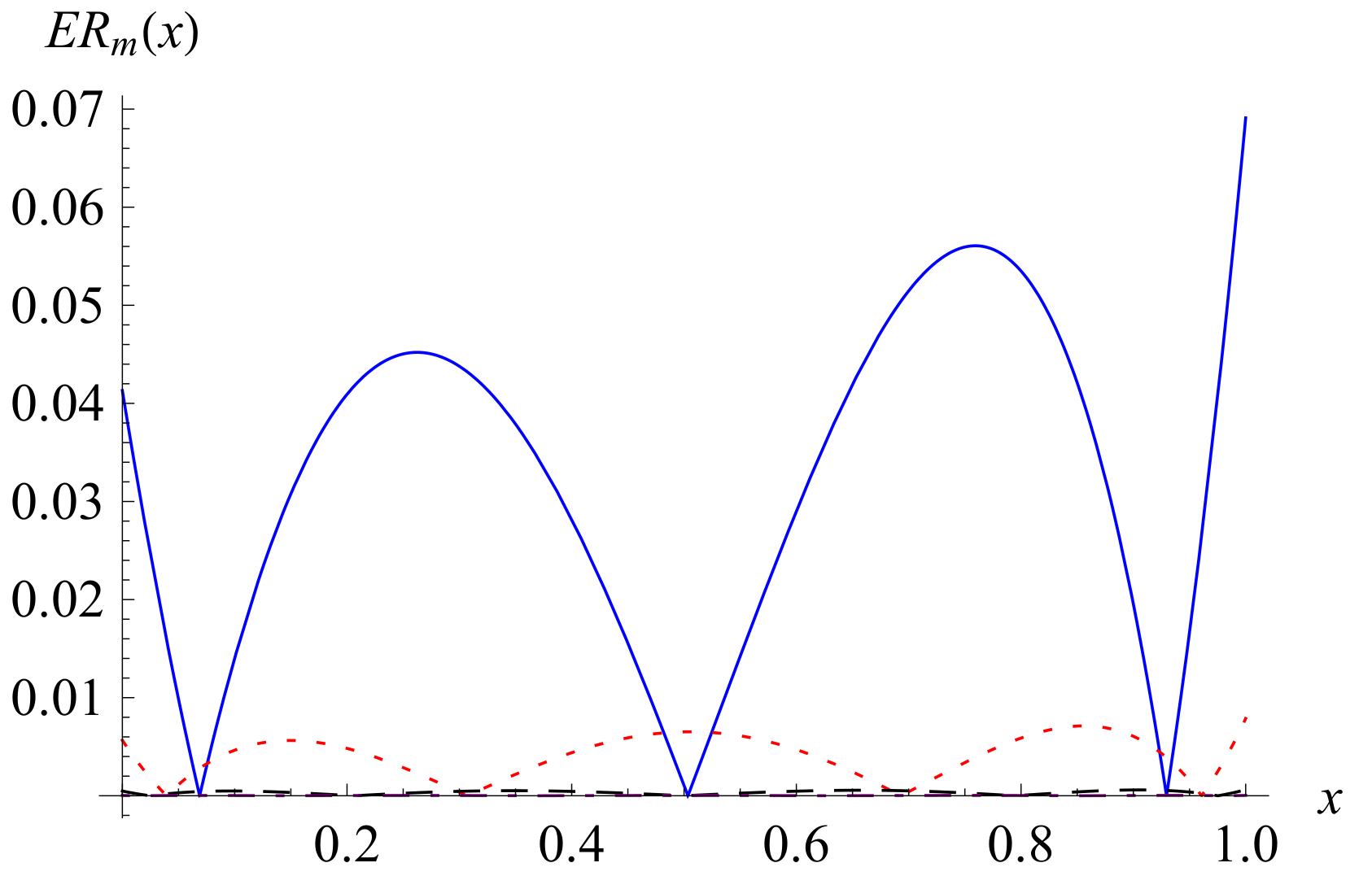
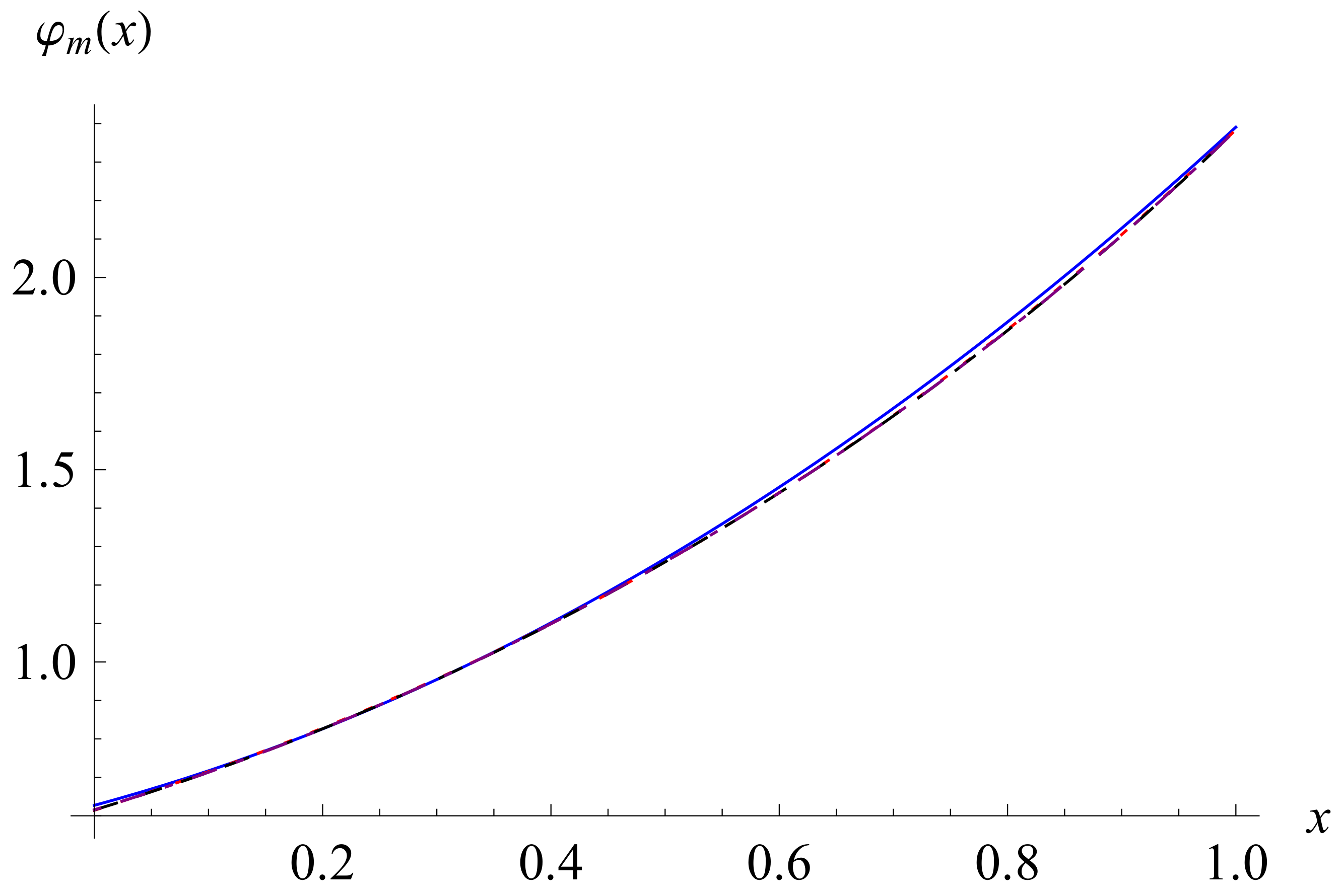
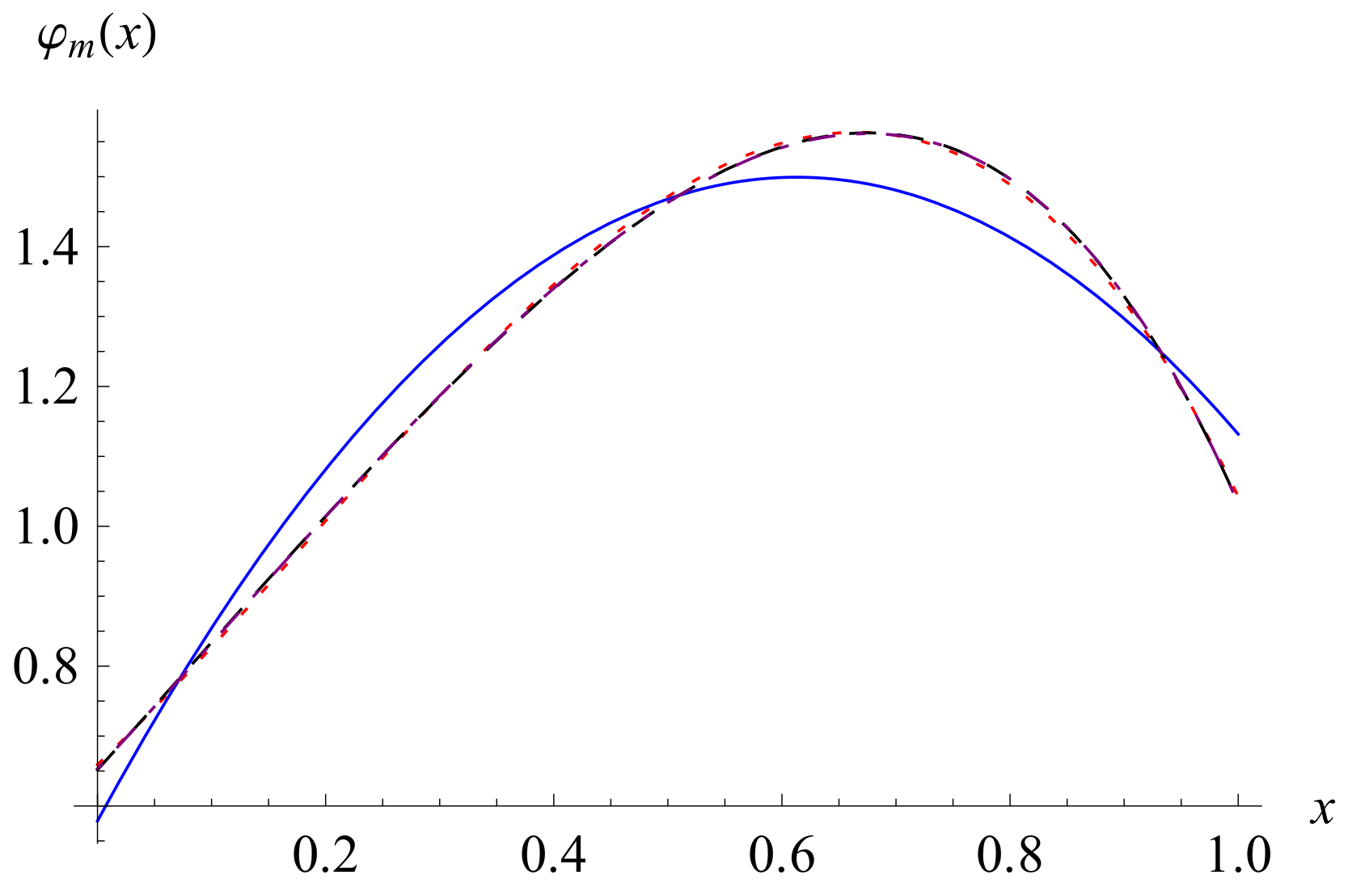
For the case of $\lambda =2$, the error functions $E{R}_m\left(x\right)=\left|{\phi }_m\left(x\right)-u^{*}\left(x\right)\right|$ are depicted in Figure 2 for m = 2–5. The maximum errors of the approximate solutions are 0.069103, 0.007877, 0.000620, and 0.000038, respectively. For the case of $\lambda =1.5$, the solution approximations ${\phi }_m\left(x\right)$, m = 2–5, are calculated as

$$\begin{array}{rrr}{\phi }_2\left(x\right)& =& 0.578503+3.00467x-2.45143x^2,\hfill \\ \hfill {\phi }_3\left(x\right)& =& 0.659109+1.56065x+1.43569x^2-2.61289x^3,\hfill \\ \hfill {\phi }_4\left(x\right)& =& 0.651626+1.81823x+0.108085x^2-0.448696x^3-1.09621x^4,\hfill \\ \hfill {\phi }_5\left(x\right)& =& 0.653112+1.75369x+0.599869x^2-1.78975x^3+0.411041x^4-0.596018x^5.\hfill \end{array}$$

Figure 2. For $\lambda =2$, the error functions $E{R}_m\left(x\right)$ for $m=2$ (solid line), $m=3$ (dot line), $m=4$ (dash line) and $m=5$ (dot-dash line).

The condition numbers of the coefficient matrices W in the derivations of the four solution approximations are 2.85, 3.29, 3.67 and 4.02, respectively. These values show that the coefficient matrices W are well conditioned. We note that the condition number is based on the $l_2$-matrix norm. The four solution approximations are plotted in Figure 3, where a fast convergence is shown.

Figure 3. For $\lambda =1.5$, the solution approximations ${\phi }_m\left(x\right)$ for $m=2$ (solid line), $m=3$ (dot line), $m=4$ (dash line) and $m=5$ (dot-dash line).

Example 3.

Consider the BVP for the linear FDE

$$\begin{array}{lll}& & D_x^{\lambda }u\left(x\right)-\frac{x}{1+x}{u}^{\prime }\left(x\right)-\frac{1}{1+x}u\left(x\right)=0,0<x<1,1<\lambda \le 2,\end{array}$$

(50)

$$\begin{array}{lll}& & u\left(0\right)-2u^{\prime }\left(0\right)=-1,u\left(1\right)+2u^{\prime }\left(1\right)=3e.\end{array}$$

(51)

If $\lambda =2$, the BVP has the exact solution $u^{*}\left(x\right)=e^x$.

The coefficients and parameters are $c_1\left(x\right)=-\frac{x}{1+x^{\prime }}$, $c_0\left(x\right)=-\frac{1}{1+x}$, $g\left(x\right)=0,$$p_0=p_1=1,q_0=q_1=2,b_0=-1,b_1=3e.$ The collocation equation system in Equation (31) becomes

$$\begin{array}{lll}& & {\displaystyle \sum _{n=0}^m}{a}_n\left(T_n^{*}\left(x_i\right)-\frac{x_i+2}{5}{I}_{x,1}^{\lambda }\left(\frac{-x}{1+x}{T_n^{*}}^{\prime }\left(x\right)+\frac{-1}{1+x}{T}_n^{*}\left(x\right)\right)\right.\\ & & -\left.\frac{2(x_i+2)}{5}{I}_{x,1}^{\lambda -1}\left(\frac{-x}{1+x}{T_n^{*}}^{\prime }\left(x\right)+\frac{-1}{1+x}{T}_n^{*}\left(x\right)\right)+I_{x,x_i}^{\lambda }\left(\frac{-x}{1+x}{T_n^{*}}^{\prime }\left(x\right)+\frac{-1}{1+x}{T}_n^{*}\left(x\right)\right)\right)=h\left(x_i\right),\hfill \end{array}$$

where $h\left(x_i\right)=\frac{1}{5}(6e-3+3e{x}_i+x_i),$$i=0,1,\dots ,m.$

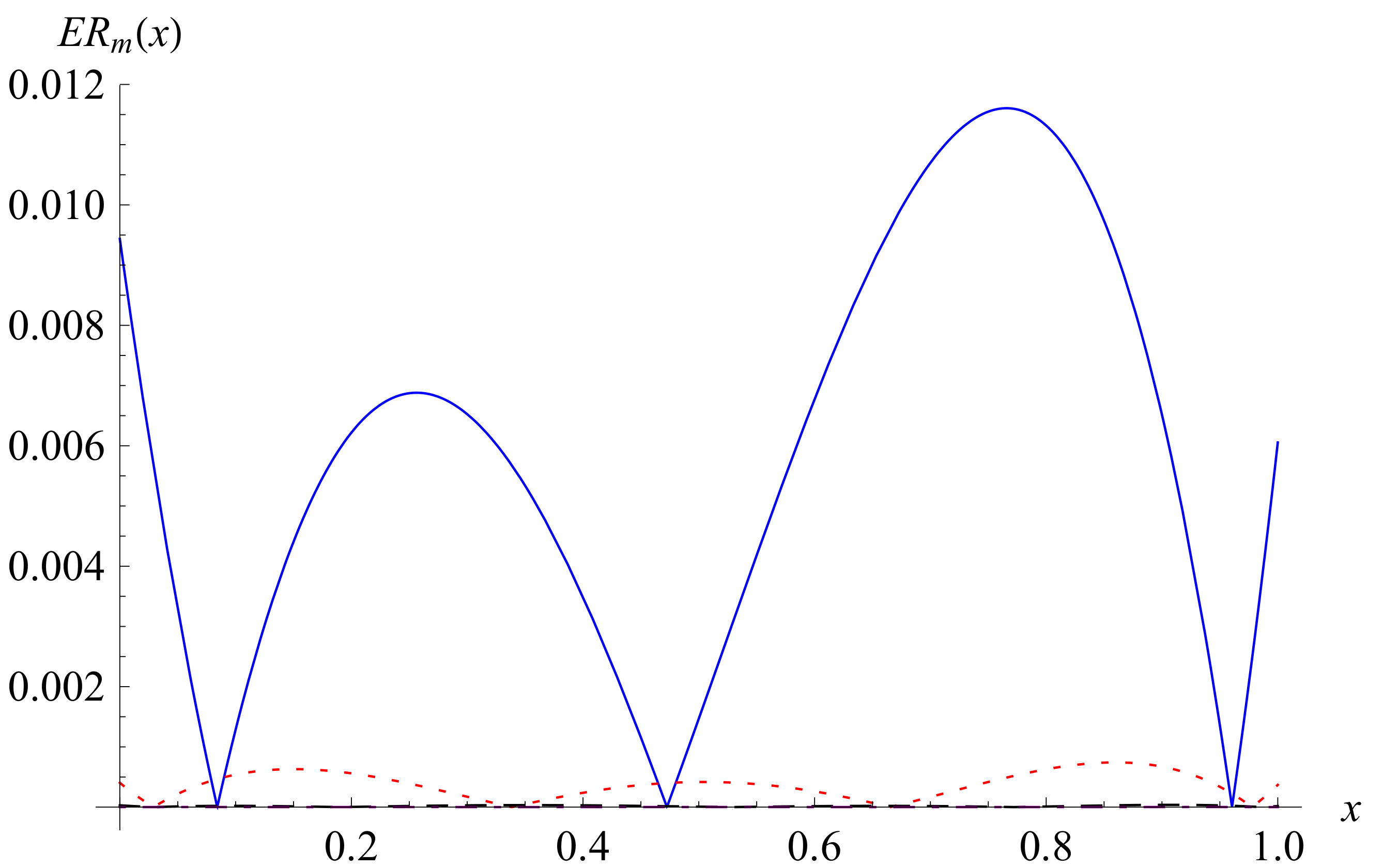
For the case of $\lambda =2$, the error functions $E{R}_m\left(x\right)=\left|{\phi }_m\left(x\right)-u^{*}\left(x\right)\right|$ for $m=2,3,4,5,$ are depicted in Figure 4. The maximum errors of the approximate solutions are 0.011605, 0.000742, 0.000037, and 0.000002, respectively. For the case of $\lambda =1.5$, the solution approximations ${\phi }_m\left(x\right)$ for $m=2,3,4,5$ are calculated as

$$\begin{array}{rrr}{\phi }_2\left(x\right)& =& 0.627196+0.801952x+0.961626x^2,\hfill \\ \hfill {\phi }_3\left(x\right)& =& 0.614413+0.94835x+0.55162x^2+0.269951x^3,\hfill \\ \hfill {\phi }_4\left(x\right)& =& 0.615168+0.908026x+0.734701x^2-0.0100847x^3+0.135331x^4,\hfill \\ \hfill {\phi }_5\left(x\right)& =& 0.615706+0.894049x+0.828159x^2-0.242103x^3+0.378859x^4-0.0913166x^5.\hfill \end{array}$$

Figure 4. For $\lambda =2$, the error functions $E{R}_m\left(x\right)$ for $m=2$ (solid line), $m=3$ (dot line), $m=4$ (dash line) and $m=5$ (dot-dash line).

The condition numbers of the coefficient matrices W in the derivations of the four solution approximations are 4.87, 7.83, 11.90 and 17.05, respectively. So the coefficient matrices W are well conditioned. The four solution approximations are plotted in Figure 5.

Figure 5. For $\lambda =1.5$, the solution approximations ${\phi }_m\left(x\right)$ for $m=2$ (solid line), $m=3$ (dot line), $m=4$ (dash line) and $m=5$ (dot-dash line).

In the three examples, fast convergent rates are shown only using the minor term number with $M=5$ in Equation (38) for the integral computation of the known functions, and the minor term number with $m=2,3,4$ and 5 in Equation (28) for the truncated Chebyshev series of the unknown function.

4. Conclusions

We considered the BVP for the varying coefficient linear Caputo-type fractional ODE subject to the mixed boundary conditions on the interval $0\le x\le 1$. The BVP was conveniently converted into an equivalent differential–integral equation merging the boundary conditions. Then, the solution was decomposed into a truncated shifted Chebyshev series. The collocation method was used to determine the solution. In order to deal with the involved integrations, the varying coefficients were again decomposed into the truncated shifted Chebyshev series. Thus, the calculations of the integrals are only for polynomials and can be carried out exactly. Three numerical examples were solved by using the proposed method, where fast convergent rates are shown only using the minor term number with $M=5$ in Equation (38) for the integral computation of the known functions, and the minor term number with $m=2,3,4$ and 5 in Equation (28) for the truncated Chebyshev series of the unknown function.

In the presented method, there is no need to divide the interval commonly used in numerical methods. The collocation points or the zeros of the Chebyshev polynomials have exact explicit expressions. Approximate analytical solutions in the polynomial forms are obtained, which are different from a discrete numerical solution. The obtained approximate analytical solutions in the polynomial forms can be directly checked by substitution. The convergence and effectiveness of solutions can be examined by remainder errors. Convergence order of the approximate solutions could be further consideration in this field.