Different Stochastic Resonances Induced by Multiplicative Polynomial Trichotomous Noise in a Fractional Order Oscillator with Time Delay and Fractional Gaussian Noise

Abstract

A general investigation on the mechanism of stochastic resonance is reported in a time-delay fractional Langevin system, which endues a nonlinear form multiplicative colored noise and fractional Gaussian noise. In terms of theoretical analysis, both the expressions of output steady-state amplitude and that of the first moment of system response are obtained by utilizing stochastic averaging method, fractional Shapiro and Laplace methods. Due to the presence of trichotomous colored noise, the excitation frequency can induce fresh multimodal Bona fide stochastic resonance, exhibiting much more novel dynamical behaviors than the non-disturbance case. It is verified that multimodal pattern only appears with small noise switching rate and memory damping order. The explicit expressions of critical noise intensity corresponding to the generalized stochastic resonance are given for the first time, by which it is determined that nonlinear form colored noise induces much more of a comprehensive resonant phenomena than the linear form. In the case of slow transfer rate noise, a newfangled phenomenon of double hypersensitive response induced by a variation in noise intensity is discovered and verified for the first time, with the necessary range of parameters for this phenomenon given. In terms of numerical scheme, an efficient and feasible algorithm for generating trichotomous noise is proposed, by which an algorithm based on the Caputo fractional derivative are applied. The numerical results match well with the analytical ones.

1. Introduction

Based on the Markov process without after-effect, classical stochastic resonance theory grounded on ordinary Langevin equation and FPE tends to be perfect gradually. However, more and more systems under complex environments exhibit memory effects, such as long-range correlation and historical dependence in time. At this time, the traditional stochastic resonance theory with ODE is obviously no longer applicable as it often needs to be modeled by non-traditional mathematical models such as fractional order differential equation. Early scholars tried to use the research method corresponding to a normal diffusion system to approximate this type of issue, e.g., fractional relaxation equation [1], fractional diffusion equation [2] and fractional Fokker–Planck equations [3]. Due to the characteristics of the fractional calculus equation itself, the systematic description of stochastic resonance in the fractional system cannot be achieved by using analytical algorithm in most cases at present.

The concept of stochastic resonance (SR) was firstly proposed in paleometeorology to explain why the climatic alternating period of warm climate and glacial period can stay in sync with the offset period of the eccentric angle of earth revolution. The synergistic effect of nonlinearity, periodic signal imposed by sun and random forces of earth itself drive the response signal cross the potential barrier, and make the climate alternation possible. However, the nonlinearity is not a necessary condition for the occurrence of stochastic resonance, say, SR can exist in linear systems disturbed by multiplicative random noise [4,5]. As research on stochastic resonance in linear systems started later than that on nonlinear systems, the former is far inferior to the latter in terms of the diversity of research methods and application range. While studies of SR in fractional systems started much later than that in integer order systems, various bistable fractional order systems are gradually taken as the main research object, and became an important topic up to the beginning of the present century. Reports on SR in linear fractional systems has been gradually developed in recent years, Ren [6] considers fractional damping fluctuations manifests as the form of trichotomous noise for the second order linear FLE, confirming that the interaction between multiplicative noise and memory effect can lead to stochastic resonance. Kim [7] analyzes self-tuning stochastic resonance energy harvesting for rotating systems under modulated noise. For all this, the stochastic resonance of linear fractional-order systems is still at the preliminary exploratory stage.

In the studies on SR of fractional order systems induced by colored noise, dichotomous and trichotomous random telephone signal (RTS) are often presented in multiplicative and additive noise terms, to describe the disturbance on oscillator mass [8], inherent frequency [9], fractional damping [10], signal modulating noise [7], etc. Due to the one-sided understanding of the complex disturbance in practical application, noises in linear form are often used to simulate the random factors for formal convenience. However, nonlinear noise exists more widely in real world systems than linear ones [11]. Many nonlinear noises such as quadratic noise [12], nonlinear Markov noise [13] and nonlinear Ornstein–Uhlenbeck noise [14] really exist in the actual physical system. As for the nonlinear dichotomous and trichotomous noise, it has attracted more and more attention on account of its universal existence and potential application in practical nonlinear physical system. On the one hand, there are research works on a variety of nonlinear noises that mainly target integer order systems, and quite a few studies involving nonlinear color noise have been reported in fractional order systems. Zhong [15] studied underdamped and overdamped fractional order systems with nonlinear color noise natural frequency disturbance, respectively. As far as we are aware, no previous work on the research of SR in second-order fractional-order anomalous diffusion systems with fractional damping disturbance of polynomial form has been reported, ever. On the other hand, on account of different propagation mechanisms, both signal and noise have a time delay effect when transmitting through the system [16], and time delays exist in many natural or artificial systems. It is found that the coexistence of noise and time delay tend to change the dynamic behavior of stochastic systems that are described by the Langevin equation [17], and this kind of synergy can also have a significant effect on the resonance phenomena [18]. Nevertheless, most studies on the effect of time delay on stochastic resonance are limited to integer order systems, and, in a numerical simulation way, analytical studies on SR for fractional order systems with time delay are quite rare. Taking all these into account, we consider a class of anomalous diffusion systems in regard to fractional Brown particles, containing small delay, fractional Gaussian internal noise, and driven by nonlinear trichotomous colored noise and external periodic excitation simultaneously.

In this paper, stochastic resonance induced by fractional damping disturbance in the form of polynomial trichotomous noise is investigated, qualitatively and quantitatively. A new feasible numerical generating algorithm for trichotomous colored noise is proposed, by which a numerical scheme for the stochastic fractional Langevin system is established. The effect of the noise switching rate and fractional damping order on the occurrence of stochastic multi-resonance is expounded, which is an exploration in the category of fractional systems with stochastic damping disturbance. In addition, some novel phenomena of hypersensitivity response are discovered, which have not been reported before, revealing the complexity in a system driven by nonlinear telegraphic noise. By this, the resonance regimes in the complex system will be understood more deeply. The organization of this paper is as follows. In Section 2, starting with the traditional Brown motion, a particle diffusion model described by the fractional Langevin equation (FLE) is introduced by virtue of the generalized Langevin equation. Section 3 is devoted to the theoretical results of the exact solution of the response, from the first moment, and the steady-state amplitude by extending the stochastic averaging method. In Section 4, detailed analysis on the bona fide stochastic resonance under different system parameter conditions are investigated. Section 5 presents the dependence of generalized stochastic resonance phenomena on time delay, noise intensity and fractional order of the damping. In Section 6 the numerical verification of the theoretical predictions is provided. The conclusion is given in the Section 7.

2. Model

In statistical thermodynamics, due to the anfractuous interaction of nonlinearity, noise and disturbances entrained in different sources, most natural systems manifest themselves as non-balanced. The modeling of stochastic systems usually focuses on part of relevant variables, and uses “random force” or “noise” with specific statistical characteristics to describe eliminated ones, with a characteristic time scale matching with the specific correlation time of the random noise [19]. When the time scale magnitude order of these eliminated variables is much smaller than that of the system’s characteristic response time, Gaussian white noise (GWN) with a pulse form correlation time can be employed for modeling. There can be practical problems, as the noises often manifest themselves into colored form with non-zero correlation time and nonconstant power spectrum. The dichotomous colored noise, which has a simple statistical property, is originally used to simulate real noise. As an extension, the trichotomous one is more flexible in modeling than the former one. In most instances, the system induced by trichotomous noise may exhibit more numerous and complicated dynamic behaviors than that induced by the dichotomous one [20].

Here we use $\zeta (t)$ to denote the ubiquitous time-continuous Markov process, which consists of shifts between three different levels, i.e., $\zeta (t)$ may jump between three values $\Delta$, $0$ and $-\Delta$, with $\Delta >0$. The jumps of this stationary random telegraph process follow, in time, according to the pattern of a Poisson process, and the stationary probability for the symmetric trichotomous noise $\zeta (t)$ at different values are

$$P_s(\zeta (t)=\Delta )=P_s(\zeta (t)=-\Delta )=p, P_s(\zeta (t)=0)=1-2p$$

(1)

thus $\zeta (t)$ would be degenerated into the dichotomous form for $p=1/2$, the conditional transition probability between the three states is determined by the master equation [21]

$$\frac{\mathrm{d}}{\mathrm{d}t}P\left({\Delta }_i,\hspace{0.17em}\hspace{0.17em}t|x,\hspace{0.33em}s\right)=v{\displaystyle \sum _{j=1}^3{A}_{ij}}P\left({\Delta }_j,\hspace{0.17em}\hspace{0.17em}t|x,\hspace{0.33em}s\right)$$

(2)

where ${\Delta }_1=\Delta$, ${\Delta }_2=0$, ${\Delta }_3=-\Delta$, $t>s$

$${\mathbf{A}}_{ij}=\left[\begin{array}{ccc}p-1& 1-2p& p\\ p& -2p& p\\ p& 1-2p& p-1\end{array}\right]$$

Combining the normalization condition ${\displaystyle \sum _{j=1}^{3}P\left({\Delta }_j,\hspace{0.17em}\hspace{0.17em}t|x,\hspace{0.33em}s\right)}=1$ and the initial conditions $P\left({\Delta }_j,\hspace{0.17em}\hspace{0.17em}t|x,\hspace{0.33em}t\right)={\delta }_{{\Delta }_{j}x}$, one can use Equation (2) to give the a probability transition matrix of noise in regard to the time interval $t-s$, and the shift between the states $\Delta$, $0$ and $-\Delta$ obey a pattern of Poisson distribution, which can be given as follows

$$\begin{array}{cc}\hfill \mathbf{P}& ={\left[P_{ij}\left(t-s\right)\right]}_{i,j\in \left\{1,2,3\right\}}={\left[P\left(\zeta \left(t\right)={\Delta }_j|\zeta \left(s\right)={\Delta }_i\right)\right]}_{i,j\in \left\{1,2,3\right\}}\hfill \\ & =\left[\begin{array}{ccc}1+\left(p-1\right)\left(1-e^{-v\left(t-s\right)}\right)& \left(1-2p\right)\left(1-e^{-v\left(t-s\right)}\right)& p\left(1-e^{-v\left(t-s\right)}\right)\\ p\left(1-e^{-v\left(t-s\right)}\right)& 1-2p\left(1-e^{-v\left(t-s\right)}\right)& p\left(1-e^{-v\left(t-s\right)}\right)\\ p\left(1-e^{-v\left(t-s\right)}\right)& \left(1-2p\right)\left(1-e^{-v\left(t-s\right)}\right)& 1+\left(p-1\right)\left(1-e^{-v\left(t-s\right)}\right)\end{array}\right]\end{array}$$

(3)

All the characters of $\zeta (t)$ are completely contained in (1) and (3), from which the mean value at arbitrary time $t$ can be calculated as

$$〈\zeta (t)|x_0,\hspace{0.17em}s〉={\displaystyle \sum _{x\in \left\{\Delta ,0,-\Delta \right\}}xP\left(x,\hspace{0.17em}t|x_0,\hspace{0.17em}s\right)}=0, t>s$$

and the autocorrelation function

$$〈\zeta \left(t\right)\zeta \left(s\right)〉={\displaystyle \sum _{x_0,x_1\in \left\{\Delta ,0,-\Delta \right\}}{x}_0{x}_{1}P\left(t,\hspace{0.17em}{x}_1|s,\hspace{0.17em}{x}_0\right)P_s\left(x_0\right)}=2p{\Delta }^2{e}^{-v\left(t-s\right)}=Dv{e}^{-v\left(t-s\right)}$$

(4)

$v$ is the switching rate, and correlation time ${\tau }_{cor}$ equals to the reciprocal of the noise switching rate

$$D={\displaystyle {\int }_0^{\infty }〈\zeta (t)\zeta (t+u)〉\mathrm{d}}u=\frac{2p{\Delta }^2}{v}, {\tau }_{cor}=\frac{1}{D}{\displaystyle {\int }_0^{+\infty }〈\zeta (t)\zeta (t+u)〉}u\mathrm{d}u=\frac{1}{v}$$

$D$ is the noise intensity. The mean square value and the counterpart mean quadruplicate value of the noise reads as $〈{\zeta }^2(t)〉=2{\Delta }^{2}p$, $〈{\zeta }^4(t)〉=2{\Delta }^{4}p$, thus one gets the flatness parameter [22] of $\zeta (t)$: $\kappa =〈{\zeta }^4(t)〉/〈{\zeta }^2(t)〉=1/2p$, $0<p<0.5$. For different $p$, $\kappa$ could be any value from one to $\infty$, and the trichotomous is reduced to a more concise case, say, the symmetric dichotomous noise and Gaussian colored noise for $\kappa =2$ and $\kappa =3$, respectively. For the other degree of freedom, it proves itself to be more flexible when modelling practical fluctuations [23].

Since the phenomenon of pollen particles’ never-ending movement in liquid was first observed by the British botanist Brown in 1827, the theory of normal diffusion based on integer ODE has been developed gradually. The model of single Brownian particle’s motion subjected to potential field force and random force in a homogeneous fluid media can be described by

$$m\frac{{\mathrm{d}}^2}{\mathrm{d}{t}^2}x\left(t\right)+m\gamma \frac{\mathrm{d}}{\mathrm{d}t}x\left(t\right)=-\frac{\mathrm{d}}{\mathrm{d}x}U\left(x\right)+\xi \left(t\right)+F\left(t\right)$$

wherein $m\gamma \dot{x}\left(t\right)$, $-\mathrm{d}U\left(x\right)/\mathrm{d}x$ and $F\left(t\right)$ represent the resistance, the potential field force, and the external force, respectively. This classical model is established on two aspects of idealized assumptions: firstly, the volume of Brownian particles is assumed to be much larger than that of fluid molecules. Since the time scale of fluid molecules’ motion is much smaller than that of Brownian particles, the association time of random forces $\xi \left(t\right)$ is extremely short, say, modeled as GWN. The second assumption is that the damping coefficient ${\gamma }_0$ should be constant, i.e., damping force at the current moment has nothing to do with t motion history. Under this Markov hypothesis, the fluid damping of Brownian particles can be determined by Stokes law, and thus can be described by the first-order derivative.

However, in practical problems many diffusion phenomena exhibit quite different pattern, e.g., solute migration in fractured lithosphere [23], anomalous diffusion in the cytoplasm of mammalian cells [24], etc. These processes can no longer be described by the standard method of statistical physics, are generally referred to as anomalous diffusion. Indeed, the abovementioned assumptions are often too idealistic, that does not correspond to the actual situation. On one hand, the size of the object particle may not be much larger than that of the impacting particles in a complex surrounding environment with nonhomogeneous media. In this case, the correlation time of collisions is no longer infinitesimal, occurrence of low-frequency collisions leads to the correlation between random forces, then the Gaussian white noise model is no longer applicable. On the other hand, in order to satisfy the characteristic equation $〈v\left(t\right)\dot{v}\left(t\right)〉=0$, the viscosity coefficient ${\gamma }_0$ should manifest as a time-dependent function ${\displaystyle {\int }_{t_0}^t\gamma \left(t-t^{\prime }\right)v\left(t^{\prime }\right)\mathrm{d}{t}^{\prime }}$ [25] rather than a constant coefficient, the damping force at any time $t$ is acquired by integrating the velocity at all times before $t$ according to the weight function $\gamma$. From the above consideration, it can be further turned into the generalized Langevin equation

$$m\frac{{\mathrm{d}}^2}{\mathrm{d}{t}^2}x\left(t\right)+m{\displaystyle {\int }_{t_0}^t\gamma \left(t-t^{\prime }\right)}\dot{x}\left(t\right)d{t}^{\prime }=-\frac{\mathrm{d}}{\mathrm{d}x}U\left(x\right)+W_H\left(t\right)$$

(5)

where $\gamma \left(t\right)$ is the memory damping kernel, describing delayed effect of the friction.

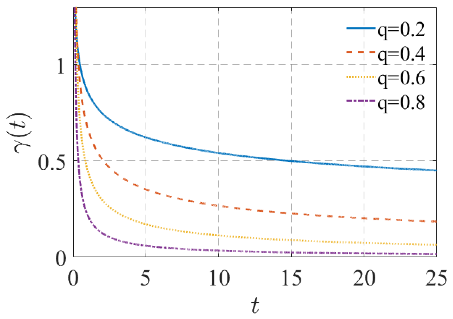
In many physical and biological environments, a power-law form memory kernel is often used to describe the dependence between viscosity force and particles’ historical velocity, as follows

$$\gamma \left(t\right)=\frac{{\gamma }_0{\left|t\right|}^{-q}}{\Gamma \left(1-q\right)}$$

(6)

The shape of damping kernel function with the friction coefficient $\delta =1$ is shown in Figure 1, it finds that $\gamma \left(t\right)$ has a power-law attenuation trend with the speed of $q$, and it would degenerate into Delta function when $q$ approach $1$. Inserting (6) into (5) and using the definition of Caputo derivative, Equation (5) can be further transformed to the following FDE

$$m\frac{{\mathrm{d}}^2}{\mathrm{d}{t}^2}x\left(t\right)+m{\gamma }_0{}_C\mathrm{D}_{0,t}^{q}x(t)=-\frac{\mathrm{d}}{\mathrm{d}x}U\left(x\right)+W_H\left(t\right)$$

(7)

The well-known Brownian motion $B(t)$ is generally used in the traditional stochastic dynamics, to model the normal diffusion with mean-square displacement (MSD) $x^2(t)=t$ induced by the random factor accompanied with all sorts of systems, it has further been confirmed to be quite serviceable in many situations. However, it is clunky when dealing with some other ubiquitous situations, i.e., the Brownian motion theory does not apply to the anomalous diffusion process [26], such as the long-range correlation behavior in history-dependent viscoelastic medium under the background of anomalous diffusion, with a magnitude of MSD the same as $t^{\alpha }$, the diffusion exponents $\alpha$ lies between zero and one for a subdiffusion situation and beyond one for a superdiffusion case, respectively [27]. By this reason, a noise with a long time memory effect is frequently adopted to describe the non-Markov dynamic behavior of anomalous diffused particles, and the correlation function of $W_H\left(t\right)$ tends to be in a power-law form, as in Equation (7) [26]. According to the fluctuation dissipation theorem [25], the friction produced by the microscopic forces of the system depends entirely on the correlation of the random forces: $〈W_H(t)W_H(s)〉=k_{B}T\gamma (\left|t-s\right|)$, with $k_B$ the Boltzmann constant and $T$ the absolute temperature. Substituting (6) into the fluctuation dissipation equality gives the power-law form autocorrelation function of random force

$$〈W_H(t)W_H(s)〉=\frac{k_{B}T{\gamma }_0{\left|t-s\right|}^{-q}}{\Gamma \left(1-q\right)}$$

(8)

Here we consider $W_H\left(t\right)$ to be the fractional Gaussian noise (FGN), and similar to the definition pattern of GWN, FGN is given by the generalized differential of the fractional Brownian motion (FBM): $W_H\left(t\right)=\sqrt{2D_H}\mathrm{d}{B}_H\left(t\right)/\mathrm{d}t$. $D_H$ denotes the noise strength, $H$ denotes the Hurst index with $0<H<1$. $B_H\left(t\right)$ is reduced to a standard Brownian motion for $H=0.5$, which has independent increments. For $H>0.5$ the increments are positively correlated, while they are negatively correlated for the opposite situation, and more details of FBM can be found in Ref. [28]. The mean value and autocorrelation function of FBM read as:

$$〈B_H\left(t\right)〉=0, 〈B_H\left(t\right)B_H\left(s\right)〉=\left(t^{2H}+s^{2H}-{\left|t-s\right|}^{2H}\right)/2,$$

where the correlation function of FGN can be obtained by the covariance of FBM

$$〈W_H(t)W_H(s)〉=2D_H\left[H(2H-1){\left|t-s\right|}^{2H-2}+2H{\left|t-s\right|}^{2H-1}\delta \left(t-s\right)\right]$$

(9)

When $t\ne s$, $0<H<1/2$ corresponds to the subdiffusion movement with a negative correlation function, $1/2<H<1$ corresponds the opposite situation, and it turns to the impulse function $〈W_H(t)W_H(s)〉=2D_H\delta \left(t-s\right)$ for $H=1/2$, say, the normal diffusion case. Utilizing the fluctuation dissipation theorem, again one gets

$$\gamma (t)=2D_{H}H(2H-1)t^{2H-2}/k_{B}T$$

(10)

The Hurst parameter should be constrained in $(0.5,\hspace{0.33em}1)$ to guarantee the mean-square value $〈W_H{}^2(t)〉$ to be positive, thus the memory kernel is positive as well. Combining (10) and (8) one has $q=2-2H$, that is, the attenuation parameters of memory kernel function correspond exactly to the order of the fractional derivative. An intensity setting of FGN as $D_H=k_{B}T{\gamma }_0/\Gamma \left(2H+1\right)$ can provide a result consistent with (6), which reveals the practical significance of considering FGN in an anomalous diffusion system.

In this paper, we consider a kind of anomalous diffusion system with small time delay $x(t-\tau )$, disturbed by nonlinear colored noise and internal FGN, which is given by the following integro-differential equation:

$$m\ddot{x}(t)+m\left\{{\gamma }_0+\Psi \left[\zeta (t),\hspace{0.17em}N\right]\right\}{\displaystyle {\int }_{t_0}^t\gamma \left(t-t^{\prime }\right)}\dot{x}\left(t\right)\mathrm{d}{t}^{\prime }+{\omega }_0{}^{2}g\left[x(t),\hspace{0.17em}x(t-\tau )\right]=A\cos \Omega t+W_H(t)$$

(11)

$\ddot{x}(t)$ and $\dot{x}\left(t\right)$ denote the acceleration and velocity, respectively. $A\cos \Omega t$ is external harmonic excitation, ${\omega }_0{}^2$ the inherent frequency. $\Psi \left[\zeta (t),\hspace{0.17em}N\right]$ ($N\ge 2$) represents the nonlinear trichotomous noise disturbance on damping intensity, which manifests itself as the polynomial form $\Psi \left[\zeta (t),\hspace{0.17em}N\right]={\displaystyle \sum _{k=1}^N{\gamma }_k{\zeta }^k(t)}$. $\zeta (t)$ is symmetric trichotomous colored noise with three states, $W_H(t)$ is zero-mean FGN with autocorrelation function given by (9) and memory damping kernel given by (6), respectively. Considering the potential field force $g(x(t),\hspace{0.17em}x(t-\tau ))=(1-\rho )x(t)+\rho x(t-\tau )$, $0\le \rho \le 1$, where $\rho$ represents delay intensity. $\rho =0$ and $\rho =1$ correspond, respectively, to non-delay and global item delay systems [17], $0<\rho <1$ corresponds to the system containing delay feedback, wherein $\rho$ is also referred as the feedback gain [29]. For computational convenience sake assume $m=1$, then based on the generalized Langevin equation given by Equation (11) and the definition of Caputo fractional derivative [30], the system can be rewritten as the following fractional Langevin equation

$$\ddot{x}(t)+\left\{{\gamma }_0+{\displaystyle \sum _{k=1}^N{\gamma }_k{\zeta }^k(t)}\right\}{}_C\mathrm{D}_{0,t}^{q}x(t)+{\omega }_0{}^2\left[(1-\rho )x(t)+\rho x(t-\tau )\right]=A\cos \Omega t+W_H(t)$$

(12)

3. Theoretical Analysis of Response

With the constructed equation $\zeta (t)(\zeta (t)-\Delta )(\zeta (t)+\Delta )=0$, and the arbitrary power of $\zeta (t)$ can be expressed by

$${\zeta }^{2m+1}(t)={\Delta }^{2m}\zeta (t), {\zeta }^{2m+2}(t)={\Delta }^{2m}{\zeta }^2(t)$$

(13)

$m$ is a positive integer, with (13) the polynomial noise in Equation (12) can be simplified to

$$\Psi (\zeta (t),\hspace{0.33em}N)={\alpha }_N\zeta (t)+{\beta }_N{\zeta }^2(t), {\alpha }_N={\displaystyle \sum _{j=1}^{⌊(N-1)/2⌋+1}{\gamma }_{2j-1}{\Delta }^{2j-2}}, {\beta }_N={\displaystyle \sum _{j=1}^{⌊N/2⌋}{\gamma }_{2j}{\Delta }^{2j-2}}$$

(14)

where “$⌊x⌋$” denotes just the value $x$ rounded down to the nearest integer. For the case of $N=1$, the effect of the linear Markovian symmetric trichotomous noise on stochastic resonance has been investigated [6]. From the expansion expression (13) it is clear that a N-order ($N>2$) polynomial trichotomous noise can be simplified to an equivalent quadratic polynomial one, i.e., the first two orders play a post role in the nonlinear trichotomous noise with arbitrary (adequate) high-level power, thus for convenience, this paper adopts the quadratic form given in (14), and all the other cases with high-power exponents can be expressed by the first two orders, thus can be discussed similarly. Moreover, for notational convenience, hereinafter the subscript “$N$” in ${\alpha }_N$ and ${\beta }_N$ will be dropped, and the simplified versions $\alpha$ and $\beta$ will be used to describe the linear coefficient and nonlinear coefficient of the polynomial function $\Psi (\zeta (t),\hspace{0.33em}N)$ of the trichotomous colored noise, respectively.

As for the function $g(x(t),\hspace{0.17em}x(t-\tau ))$ of the small time delay, when $\rho =0$ no delay appeared, and this mainstream situation has attracted widespread attention. Meanwhile the global delay case happens for $\rho =1$ and the stiffness term disappears [15,17]. The scenario of $0<\rho <1$ refers to the time-delayed feedback in the system [29], the small time-delay pre-assumption enables us to expand the small delay approximation method (SDAM) [31] to the current fractional system case, say, $g(x(t),\hspace{0.17em}x(t-\tau ))$ and can be expressed as a Taylor expansion series with respect to the time delay around $x(t)$, with the convergence precision the same order of magnitude as $O({\tau }^2)$. In fact, such a Taylor expansion approximation of a function with respect to $x(t)$ has been proved workable when dealing with a small delay term, no matter whether in an integer-order differential system [32] or a fractional-order system [33]. Making use of this approximation method, one gets:

$${\omega }_0{}^{2}g(x(t),\hspace{0.17em}x(t-\tau ))\approx {\tilde{\omega }}_0{}^{2}x(t)$$

(15)

where ${\tilde{\omega }}_0{}^2={\omega }_0{}^2\left[1-\tau \rho {\omega }_0{}^2\right]$.

Combining Equation (15) and, as discussed below, Equation (14), we obtain a non-delayed stochastic differential equation, which is equivalent to Equation (12):

$$\frac{{\mathrm{d}}^2}{\mathrm{d}{t}^2}x(t)+\left[{\gamma }_0+\alpha \zeta (t)+\beta {\zeta }^2(t)\right]{\mathrm{D}}^{q}x(t)+{\tilde{\omega }}_0{}^{2}x(t)=A\cos (\Omega t)+{\eta }_H(t)$$

(16)

As mentioned above in Introduction section, there are many alternative assessment indexes to quantify the SR phenomenon in stochastic systems. Among them, the amplitude gain of the output signal is often considered as the one that could be utilized the most, from an analytical point of view. When describing the generalized SR and bona fide one, naturally many researchers have adopted this index in dealing with SR problems for its simplicity and effectiveness in practice. In this paper an analytical expression of the amplitude gain of the output signal in regard to the system given by Equation (12) will be discussed in detail, however, before doing this, we first calculate the exact solution of the first-order moment of the fractional system. This operation is feasible since the displacement process $〈x(t)〉$ could be always stationary [33]. In fact, the fractional particle in Equation (12) will always be pulled back to the origin sooner or later due to the existence of the harmonic potential $V(x)=({\tilde{\omega }}_0{}^2{x}^2)/2$. For this purpose, the Shapiro–Loginov formula [8] should be taken account for the exponential correlative trichotomous process:

$$\frac{\mathrm{d}}{\mathrm{d}t}〈\zeta (t)x(t)〉=〈\zeta (t)\frac{\mathrm{d}}{\mathrm{d}t}x(t)〉-v〈\zeta (t)x(t)〉,$$

and the fractional Shapiro-Loginov formula:

$$〈\zeta (t){\mathrm{D}}^{q}x(t)〉=e^{-vt}{\mathrm{D}}^q\left(〈\zeta (t)x(t)〉e^{vt}\right)$$

(17)

Here, $x(t)$ is considered as a function of $\zeta (t)$. Taking average of Equation (16), one gets

$$\left(\frac{{\mathrm{d}}^2}{\mathrm{d}{t}^2}+{\tilde{\omega }}_0{}^2+{\gamma }_0{\mathrm{D}}^q\right)〈x(t)〉+\alpha 〈\zeta (t){\mathrm{D}}^{q}x(t)〉+\beta 〈{\zeta }^2(t){\mathrm{D}}^{q}x(t)〉=A\cos (\Omega t)$$

(18)

The prerequisite condition $〈{\eta }_H(t)〉=0$ has been used in Equation (18), considering the properties of the trichotomous noise and using the transition probabilities and stationary probabilities, the mean-square value and the correlation function of ${\zeta }^2(t)$ are given by $〈{\zeta }^2(t)〉=2{\Delta }^{2}p$ and

$$\begin{array}{ll}\langle {\zeta }^2(t){\zeta }^2(t+\Delta t)\rangle & {\displaystyle =\sum _{\begin{array}{l}{z}_1\in \left\{-\Delta ,\Delta \right\}\\ z_2\in \left\{-\Delta ,\Delta \right\}\end{array}}{\Delta }^{4}P\left(\zeta (t+\tau )=z_2|\zeta (t)=z_1\right)P_s(\zeta (t)=z_1)}\\ & =4p{\Delta }^4+2p^2{\Delta }^4(1-2p)e^{-v△t}\end{array}$$

It is apparent from the above autocorrelation function of the mean value $〈{\zeta }^2(t)〉$ that ${\zeta }^2(t)$ does not satisfy the conditions of the Shapiro–Loginov formula, however, the situation becomes gratifying for the adjustive variable ${\zeta }^2(t)-2{\Delta }^{2}p$, that

$$\left\{\begin{array}{l}〈{\zeta }^2(t)-2{\Delta }^{2}p〉=0\hfill \\ 〈\left({\zeta }^2(t)-2{\Delta }^{2}p\right)\left({\zeta }^2(t+△t)-2{\Delta }^{2}p\right)〉=2p^2{\Delta }^4(1-2p)e^{-v△t}\hfill \end{array}\right.$$

Thus, the random variable ${\zeta }^2(t)-2{\Delta }^{2}p$ is applicable for various kinds of Shapiro–Loginov formulas (of course also including the fractional version (3.5))

$$\begin{array}{l}〈({\zeta }^2(t)-2{\Delta }^{2}p){\mathrm{D}}^{q}x(t)〉=e^{-vt}{\mathrm{D}}^q\left[〈({\zeta }^2(t)-2{\Delta }^{2}p)x(t)〉e^{vt}\right]\\ \hspace{1em}\hspace{1em}\hspace{1em}\hspace{1em}\hspace{1em}\hspace{1em}\hspace{1em}\hspace{1em}\hspace{1em}\hspace{0.33em}\hspace{0.33em}\hspace{0.33em}=〈{\zeta }^2(t){\mathrm{D}}^{q}x(t)〉-2{\Delta }^{2}p{\mathrm{D}}^q〈x(t)〉\end{array}$$

(19)

(19) leads to the new correlation factor $〈{\zeta }^2(t){\mathrm{D}}^{q}x(t)〉$ appear in (18):

$$〈{\zeta }^2(t){\mathrm{D}}^{q}x(t)〉=2p{\Delta }^2{\mathrm{D}}^q〈x(t)〉+e^{-vt}{\mathrm{D}}^q\left[\left(〈{\zeta }^2(t)x(t)〉-2{\Delta }^{2}p〈x(t)〉\right)e^{vt}\right]$$

(20)

By substituting Equations (17) and (20) into (18), one gets the equation

$$\begin{array}{l}\left(\frac{{\mathrm{d}}^2}{\mathrm{d}{t}^2}+{\tilde{\omega }}_0{}^2\right)〈x〉+\left({\gamma }_0+2p{\Delta }^2\beta \right){\mathrm{D}}^q〈x〉+\alpha e^{-vt}{\mathrm{D}}^q\left(〈\zeta x〉e^{vt}\right)+\\ \beta e^{-vt}{\mathrm{D}}^q\left(〈{\zeta }^{2}x〉e^{vt}\right)-2p{\Delta }^2\beta e^{-vt}{\mathrm{D}}^q\left(〈x〉e^{vt}\right)=A\cos (\Omega t)\end{array}$$

(21)

To solve the new factor $〈\zeta (t)x(t)〉$, multiplying Equation (16) by $\zeta (t)$ and averaging over the gained equation, one arrives at

$$〈\zeta \frac{{\mathrm{d}}^2}{\mathrm{d}{t}^2}x〉+{\gamma }_0〈\zeta {\mathrm{D}}^{q}x〉+\alpha 〈{\zeta }^2{\mathrm{D}}^{q}x〉+\beta 〈{\zeta }^3{\mathrm{D}}^{q}x〉+{\tilde{\omega }}_0{}^2〈\zeta x〉=0$$

(22)

in Equation (22) the uncorrelated postulate between $\zeta \left(t\right)$ and the FGN ${\eta }_H\left(t\right)$ has already been adopted, i.e., $〈{\zeta }^k(t){\eta }_H\left(s\right)〉=0$, $k=1,\hspace{0.17em}2\dots$ Reusing the Shapiro–Loginov formula, we have

$$〈\zeta (t)\frac{{\mathrm{d}}^2}{\mathrm{d}{t}^2}x(t)〉=\frac{{\mathrm{d}}^2}{\mathrm{d}{t}^2}〈\zeta (t)x(t)〉+2v\frac{\mathrm{d}}{\mathrm{d}t}〈\zeta (t)x(t)〉+v^2〈\zeta (t)x(t)〉$$

(23)

Substituting (17), (20) and (23) into Equation (22) yields

$$\begin{array}{l}\left[{\left(\frac{\mathrm{d}}{\mathrm{d}t}+v\right)}^2+{\tilde{\omega }}_0{}^2\right]〈\zeta x〉+2p{\Delta }^2\alpha {\mathrm{D}}^q〈x〉+\left({\gamma }_0+\beta {\Delta }^2\right)e^{-vt}{\mathrm{D}}^q\left(〈\zeta x〉e^{vt}\right)\\ +\alpha e^{-vt}{\mathrm{D}}^q\left(〈{\zeta }^{2}x〉e^{vt}\right)-2p{\Delta }^2\alpha e^{-vt}{\mathrm{D}}^q\left(〈x〉e^{vt}\right)=0\end{array}$$

(24)

In order to solve the term $〈{\zeta }^{2}x〉$, multiplying Equation (16) by ${\zeta }^2(t)$ and the averaging the gained results, one obtains:

$$〈{\zeta }^2\frac{{\mathrm{d}}^2}{\mathrm{d}{t}^2}x〉+{\gamma }_0〈{\zeta }^2{\mathrm{D}}^{q}x〉+\alpha 〈{\zeta }^3{\mathrm{D}}^{q}x〉+\beta 〈{\zeta }^4{\mathrm{D}}^{q}x〉+{\tilde{\omega }}_0{}^2〈{\zeta }^{2}x〉=2p{\Delta }^{2}A\cos (\Omega t)$$

(25)

the first averaged term in Equation (25) can also be derived by (19) and (23)

$$\begin{array}{l}〈\left({\zeta }^2-2p{\Delta }^2\right)\frac{{\mathrm{d}}^2}{\mathrm{d}{t}^2}x〉=\frac{{\mathrm{d}}^2}{\mathrm{d}{t}^2}〈\left({\zeta }^2-2p{\Delta }^2\right)x〉+2v\frac{\mathrm{d}}{\mathrm{d}t}〈\left({\zeta }^2-2p{\Delta }^2\right)x〉\\ \hspace{0.33em}+v^2〈\left({\zeta }^2-2p{\Delta }^2\right)x〉=〈{\zeta }^2\frac{{\mathrm{d}}^2}{\mathrm{d}{t}^2}x〉-2p{\Delta }^2\frac{{\mathrm{d}}^2}{\mathrm{d}{t}^2}〈x〉\end{array}$$

(26)

From (26) the averaging value $〈{\zeta }^2\frac{{\mathrm{d}}^2}{\mathrm{d}{t}^2}x〉$ can be obtained as the expression

$$〈{\zeta }^2\frac{{\mathrm{d}}^2}{\mathrm{d}{t}^2}x〉=\frac{{\mathrm{d}}^2}{\mathrm{d}{t}^2}〈{\zeta }^{2}x〉+2v\frac{\mathrm{d}}{\mathrm{d}t}〈{\zeta }^{2}x〉+v^2〈{\zeta }^{2}x〉-4p{\Delta }^{2}v\frac{\mathrm{d}}{\mathrm{d}t}〈x〉-2p{\Delta }^2{v}^2〈x〉$$

(27)

Inserting (17), (20) and (27) into Equation (25), meanwhile, replacing ${\zeta }^3(t)$, ${\zeta }^4(t)$ for ${\Delta }^2\zeta (t)$ and ${\Delta }^2{\zeta }^2(t)$, respectively, then (27) can be transformed to

$$\begin{array}{l}\left[{\left(\frac{\mathrm{d}}{\mathrm{d}t}+v\right)}^2+{\tilde{\omega }}_0{}^2\right]〈{\zeta }^{2}x〉-4p{\Delta }^{2}v\frac{\mathrm{d}}{\mathrm{d}t}〈x〉-2p{\Delta }^2{v}^2〈x〉+\\ \left(2p{\Delta }^2{\gamma }_0+2p{\Delta }^4\beta \right){\mathrm{D}}^q〈x〉+\alpha {\Delta }^2{e}^{-vt}{\mathrm{D}}^q\left(〈\zeta x〉e^{vt}\right)+\left({\gamma }_0+\beta {\Delta }^2\right)e^{-vt}{\mathrm{D}}^q\left(〈{\zeta }^{2}x〉e^{vt}\right)\\ -\left(2p{\Delta }^2{\gamma }_0+2p{\Delta }^4\beta \right)e^{-vt}{\mathrm{D}}^q\left(〈x〉e^{vt}\right)=2p{\Delta }^{2}A\cos (\Omega t)\end{array}$$

(28)

the harmonic terms on the right side of Equation (28) would not further be eliminated unless recurring to Equation (21), in fact, multiplying Equation (21) by $2p{\Delta }^2$ and subtracting the gained equation from Equation (28), one can obtain:

$$\begin{array}{l}\left[{\left(\frac{\mathrm{d}}{\mathrm{d}t}+v\right)}^2+{\tilde{\omega }}_0{}^2\right]〈{\zeta }^{2}x〉+\left({\gamma }_0+\beta {\Delta }^2-2p{\Delta }^2\beta \right)e^{-vt}{\mathrm{D}}^q\left(〈{\zeta }^{2}x〉e^{vt}\right)\\ +\alpha {\Delta }^2\left(1-2p\right)e^{-vt}{\mathrm{D}}^q\left(〈\zeta x〉e^{vt}\right)+2p{\Delta }^2\left[\beta {\Delta }^2\left(2p-1\right)-{\gamma }_0\right]e^{-vt}{\mathrm{D}}^q\left(〈x〉e^{vt}\right)\\ +2p{\Delta }^4\beta \left(1-2p\right){\mathrm{D}}^q〈x〉-2p{\Delta }^2\left(v^2+{\tilde{\omega }}_0{}^2\right)〈x〉-4p{\Delta }^{2}v\frac{\mathrm{d}}{\mathrm{d}t}〈x〉-2p{\Delta }^2\frac{{\mathrm{d}}^2}{\mathrm{d}{t}^2}〈x〉=0\end{array}$$

(29)

The collection of (21), (24) and (29) truly consists of a close linear system of second-order differential equations for three variables $m_1(t)=〈x(t)〉$, $m_2(t)=〈\zeta (t)x(t)〉$, $m_3(t)=〈{\zeta }^2(t)x(t)〉$. By virtue of the Laplace transform technique, this equation set can be equivalently changed to a corresponding linear algebraic equation set, given as follows

$$\left\{\begin{array}{l}{a}_{11}{M}_1+a_{12}{M}_2+a_{13}{M}_3=As/\left(s^2+{\Omega }^2\right)+{m^{\prime }}_1(0)+b_{11}{m}_1(0)+b_{12}{m}_2(0)+b_{13}{m}_3(0)\hfill \\ a_{21}{M}_1+a_{22}{M}_2+a_{23}{M}_3={m^{\prime }}_2(0)+b_{21}{m}_1(0)+b_{22}{m}_2(0)+b_{23}{m}_3(0)\hfill \\ a_{31}{M}_1+a_{32}{M}_2+a_{33}{M}_3={m^{\prime }}_3(0)-2p{\Delta }^2{m^{\prime }}_1(0)+b_{31}{m}_1(0)+b_{32}{m}_2(0)+b_{33}{m}_3(0)\hfill \end{array}\right.$$

(30)

$$\begin{array}{c}{a}_{11}=s^2+{\tilde{\omega }}_0^2+({\gamma }_0+2p{\Delta }^2\beta )s^q-2p{\Delta }^2\beta {(s+v)}^q, a_{12}=\alpha {(s+v)}^q, a_{13}=\beta {(s+v)}^q, \hfill \\ a_{21}=2p{\Delta }^2\alpha \left[s^q-{(s+v)}^q\right], a_{22}={(s+v)}^2+{\tilde{\omega }}_0^2+({\gamma }_0+\beta {\Delta }^2){(s+v)}^q, a_{23}=a_{12}, \hfill \\ a_{31}=-2p{\Delta }^2\left\{{\tilde{\omega }}_0^2+{\left(s+v\right)}^2+{\gamma }_0{\left(s+v\right)}^q+\beta {\Delta }^2\left(1-2p\right)\left[{\left(s+v\right)}^q-s^q\right]\right\}\hfill \\ a_{32}={\Delta }^2(1-2p)\alpha {(s+v)}^q, a_{33}={(s+v)}^2+{\tilde{\omega }}_0^2+({\gamma }_0+\beta {\Delta }^2-2p{\Delta }^2\beta ){(s+v)}^q, \hfill \\ b_{11}=s+({\gamma }_0+2p{\Delta }^2\beta )s^{q-1}-2p{\Delta }^2\beta {(s+v)}^{q-1}, b_{12}=\alpha {(s+v)}^{q-1}, b_{13}=\beta {(s+v)}^{q-1}, \hfill \\ b_{21}=2p{\Delta }^2\alpha \left[s^{q-1}-{(s+v)}^{q-1}\right], b_{22}=s+2v+({\gamma }_0+\beta {\Delta }^2){(s+v)}^{q-1}, b_{23}=b_{12}, \hfill \\ b_{31}=2p{\Delta }^2\left[\beta {\Delta }^2\left(2p-1\right)-{\gamma }_0\right]{\left(s+v\right)}^{q-1}+2p\beta {\Delta }^4\left(1-2p\right)s^{q-1}-4p{\Delta }^{2}v-2p{\Delta }^{2}s, \hfill \\ b_{32}={\Delta }^2(1-2p)\alpha {(s+v)}^{q-1}, b_{33}=s+2v+({\gamma }_0+\beta {\Delta }^2-2p{\Delta }^2\beta ){(s+v)}^{q-1}.\hfill \\ M_k(s)=ℒ\left(m_k(t)\right)={\displaystyle {\int }_0^{\infty }{m}_k(t)\cdot e^{-st}\mathrm{d}t}, k\in \left\{1,2,3\right\}. \hfill \end{array}$$

Displacement’s first-order moment can be formally expressed formally as bellow:

$$M_1(s)={\tilde{H}}_{10}(s)\frac{As}{s^2+{\Omega }^2}+{\displaystyle \sum _{k=1}^3{\tilde{H}}_{1k}(s)m_k(0)}+{\displaystyle \sum _{k=1}^3{\tilde{G}}_{1k}(s){m^{\prime }}_k(0)}$$

(31)

$$\begin{gathered} {\tilde{H}}_{10}(s)=\left(a_{22}{a}_{33}-a_{23}{a}_{32}\right)/I\left(s\right), \\ {\tilde{H}}_{11}(s)=\left(b_{11}{a}_{22}{a}_{33}-b_{11}{a}_{23}{a}_{32}+a_{13}{b}_{21}{a}_{32}-a_{12}{b}_{21}{a}_{33}+a_{12}{a}_{23}{b}_{31}-a_{13}{a}_{22}{b}_{31}\right)/I\left(s\right) \\ {\tilde{H}}_{12}(s)=\left(b_{12}{a}_{22}{a}_{33}-b_{12}{a}_{23}{a}_{32}+a_{13}{b}_{22}{a}_{32}-a_{12}{b}_{22}{a}_{33}+a_{12}{a}_{23}{b}_{32}-a_{13}{a}_{22}{b}_{32}\right)/I\left(s\right) \\ {\tilde{H}}_{13}(s)=\left(b_{13}{a}_{22}{a}_{33}-b_{13}{a}_{23}{a}_{32}+a_{13}{b}_{23}{a}_{32}-a_{12}{b}_{23}{a}_{33}+a_{12}{a}_{23}{b}_{33}-a_{13}{a}_{22}{b}_{33}\right)/I\left(s\right) \\ {\tilde{G}}_{11}(s)=\left(a_{22}{a}_{33}-a_{23}{a}_{32}+2p{\Delta }^2(a_{13}{a}_{22}-a_{12}{a}_{23})\right)/I(s) \\ {\tilde{G}}_{12}(s)=\left(a_{13}{a}_{32}-a_{12}{a}_{33}\right)/I\left(s\right), {\tilde{G}}_{13}(s)=\left(a_{12}{a}_{23}-a_{13}{a}_{22}\right)/I\left(s\right) \\ I(s)=a_{11}{a}_{22}{a}_{33}+a_{12}{a}_{23}{a}_{31}+a_{13}{a}_{21}{a}_{32}-a_{13}{a}_{22}{a}_{31}-a_{11}{a}_{23}{a}_{32}-a_{12}{a}_{21}{a}_{33} \end{gathered}$$

(32)

Applying the inverse Laplace transformation technique on Equation (31) and based on the corresponding uniqueness condition [34], the averaging mean value (the first-order moment) of the displacement of Equation (12) can be represented in the following form:

$$〈x(t)〉=A{H}_{10}(t)\ast \cos (\Omega t)+{\displaystyle \sum _{k=1}^3{H}_{1k}(t)m_k(0)}+{\displaystyle \sum _{k=1}^3{G}_{1k}(t){m^{\prime }}_k(0)}$$

(33)

“$\ast$” the convolution operation, $H_{10}(t)={ℒ}^{-1}\left({\tilde{H}}_{10}(s)\right)$, $H_{1k}(t)={ℒ}^{-1}\left({\tilde{H}}_{1k}(s)\right)$, $G_{1k}(t)={ℒ}^{-1}\left({\tilde{G}}_{1k}(s)\right)$, with the inverse Laplace operator the primitive function $y(t)$ can be calculated by the integral of its corresponding Laplace transformation function $Y(s)$: $y(t)={ℒ}^{-1}\left(Y(s)\right)=\frac{1}{2\pi i}{\displaystyle {\int }_{\epsilon -i\infty }^{\epsilon +i\infty }Y(s)}{e}^{st}\mathrm{d}s$.

Based on the stability theory [35], the stability of the solution expressed as (33) can be guaranteed under the circumstances that all the possible solutions of the equation $I(s)=0$ have roots with a negative or zero real part. When considering the asymptotic behavior of the functions on the right hand of (33), i.e., at a long-time limit $t\to \infty$, by making use of the Tauberian theorem [36], one gets the estimation: $H_{10}(t)=O(t^{-q})$, $H_{1k}(t)$, $G_{1k}(t)=O(t^{-(1+q)})$, thus the memorizing effect of the initial conditions can be disregarded when the system has a long enough evolute, i.e., the stationary solution of the first-order moment of the displacement in a system described by Equation (12) can be obtained by (33).

$${〈x(t)〉}_{as}=A{\displaystyle {\int }_0^t{H}_{10}(t-t^{\prime })}\cos (\Omega t^{\prime })\mathrm{d}{t}^{\prime }$$

(34)

the complex susceptibility of the stochastic system given by Equation (12) can be given based on the form of (34) [37]: $\aleph (\Omega )={\displaystyle {\int }_0^{\infty }{H}_{10}(t)e^{i\Omega t}}\mathrm{d}t=H(-i\Omega )={\aleph }_1(\Omega )+{\aleph }_2(\Omega )\cdot i$, where $i$ denotes the imaginary unit with $i^2=-1$, ${\aleph }_1$ and ${\aleph }_2$ representing the real and imaginary parts of the complex susceptibility, respectively. Moreover, with the help of the linear response theory [38], (34) can be rewritten in the following harmonic pattern as well ${〈x(t)〉}_{as}=F\cos (\Omega t+\varphi )$. With the output amplitude $F=A/\left|\aleph \right|$ and the phase shift given as, $\varphi =\arctan (-{\aleph }_2/{\aleph }_1)$, it is worth nothing that ${\tilde{H}}_{10}(i\Omega )=\overline{{\tilde{H}}_{10}(-i\Omega )}=\overline{\aleph }={\aleph }_1-{\aleph }_{2}i$, thus $F$ and $\varphi$ can also be calculated by $F=A\left|{\tilde{H}}_{10}(i\Omega )\right|$, $\varphi =\arg ({\tilde{H}}_{10}(i\Omega ))$. The response amplitude gain, say, the ratio of the amplitude of the output signal to the amplitude of input signal, then can be expressed as

$$R=\frac{F}{A}=\left|{\tilde{H}}_{10}(i\Omega )\right|$$

Through the expressions of the transfer function given in (31) and the coefficients below (29), after a series of simplification calculations, one can obtain

$$R=\sqrt{\frac{e_1{}^2+e_2{}^2}{e_3{}^2+e_4{}^2}}, \varphi =\arctan (\frac{e_2{e}_3-e_1{e}_4}{e_1{e}_3+e_2{e}_4}),$$

(35)

where $e_k$, $k=1,\dots ,4$ are listed as follows:

$$\begin{array}{c}{e}_1={\tilde{\omega }}_0{}^4+B^4\cos (4\theta )+2{\tilde{\omega }}_0{}^2{B}^2\cos (2\theta )+{\tilde{\omega }}_0{}^2{J}_1{B}^q\cos (q\theta )+J_1{B}^{q+2}\cos \left[\left(q+2\right)\theta \right]+J_2{B}^{2q}\cos (2q\theta )\hfill \\ e_2=B^4\sin (4\theta )+2{\tilde{\omega }}_0{}^2{B}^2\sin (2\theta )+{\tilde{\omega }}_0{}^2{J}_1{B}^q\sin (q\theta )+J_1{B}^{q+2}\sin \left[\left(q+2\right)\theta \right]+J_2{B}^{2q}\sin (2q\theta )\hfill \\ +\left[J_2{J}_3+{\tilde{\omega }}_0{}^2{J}_5\left({\alpha }^2-\beta J_1-J_6-\beta J_7\right)\right]B^{2q}\cos (2q\theta )+J_5\left[{\gamma }_0{\alpha }^2+J_6{J}_7-\beta J_2\right]B^{3q}\cos (3q\theta )\hfill \\ +J_1{J}_3{B}^{q+2}\cos \left[\left(q+2\right)\theta \right]+\left(J_1{J}_4-{\alpha }^2{\Omega }^q{J}_5-\beta J_5{J}_8\right)B^{q+2}\cos \left[\left(q+2\right)\theta +\frac{\pi }{2}q\right]\hfill \\ {\tilde{\omega }}_0{}^2\left(J_1{J}_4-{\alpha }^2{\Omega }^q{J}_5-\beta J_5{J}_8\right)B^q\cos \left[\left(\theta +\frac{\pi }{2}\right)q\right]+J_5\left({\alpha }^2-\beta J_1-J_6-\beta J_7\right)B^{2q+2}\cos \left[\left(2q+2\right)\theta \right]\hfill \\ +\left(J_2{J}_4-{\gamma }_0{\alpha }^2{\Omega }^q{J}_5+J_5{J}_6{J}_8\right)B^{2q}\cos \left[\left(2\theta +\frac{\pi }{2}\right)q\right]+2{\tilde{\omega }}_0{}^2{J}_4{B}^2\cos (2\theta +\frac{\pi }{2}q)\hfill \\ +J_4{B}^4\cos (4\theta +\frac{\pi }{2}q)\hfill \\ e_4=2{\tilde{\omega }}_0{}^2{B}^2{J}_3\sin (2\theta )+B^4{J}_3\sin (4\theta )+{\tilde{\omega }}_0{}^2{J}_1{J}_3{B}^q\sin (q\theta )+{\tilde{\omega }}_0{}^4{J}_4\sin (\frac{\pi }{2}q)\hfill \\ +\left[J_2{J}_3+{\tilde{\omega }}_0{}^2{J}_5\left({\alpha }^2-\beta J_1-J_6-\beta J_7\right)\right]B^{2q}\sin (2q\theta )+J_5\left[{\gamma }_0{\alpha }^2+J_6{J}_7-\beta J_2\right]B^{3q}\sin (3q\theta )\hfill \\ +J_1{J}_3{B}^{q+2}\sin \left[\left(q+2\right)\theta \right]+\left(J_1{J}_4-{\alpha }^2{\Omega }^q{J}_5-\beta J_5{J}_8\right)B^{q+2}\sin \left[\left(q+2\right)\theta +\frac{\pi }{2}q\right]\hfill \\ {\tilde{\omega }}_0{}^2\left(J_1{J}_4-{\alpha }^2{\Omega }^q{J}_5-\beta J_5{J}_8\right)B^q\sin \left[\left(\theta +\frac{\pi }{2}\right)q\right]+J_5\left({\alpha }^2-\beta J_1-J_6-\beta J_7\right)B^{2q+2}\sin \left[\left(2q+2\right)\theta \right]\hfill \\ +\left(J_2{J}_4-{\gamma }_0{\alpha }^2{\Omega }^q{J}_5+J_5{J}_6{J}_8\right)B^{2q}\sin \left[\left(2\theta +\frac{\pi }{2}\right)q\right]+2{\tilde{\omega }}_0{}^2{J}_4{B}^2\sin (2\theta +\frac{\pi }{2}q)\hfill \\ +J_4{B}^4\sin (4\theta +\frac{\pi }{2}q)\hfill \\ B=\sqrt{v^2+{\Omega }^2},\theta =\arctan (\frac{\Omega }{v}),\hfill \\ J_1=2\left({\gamma }_0-\beta {\Delta }^2-p\beta {\Delta }^2\right)\hfill \\ J_2=\left({\gamma }_0+\beta {\Delta }^2\right)\left({\gamma }_0+\beta {\Delta }^2-2p\beta {\Delta }^2\right)-{\Delta }^2\left(1-2p\right){\alpha }^2,J_3={\tilde{\omega }}_0{}^2-{\Omega }^2,J_4=\left({\gamma }_0+2p{\Delta }^2\beta \right){\Omega }^q,\hfill \\ J_5=2p{\Delta }^2,J_6={\alpha }^2-{\gamma }_0\beta -{\beta }^2{\Delta }^2,J_7=2p\beta {\Delta }^2-\beta {\Delta }^2-{\gamma }_0,J_8=\beta {\Delta }^2\left(1-2p\right){\Omega }^q.\hfill \end{array}$$

4. Bona Fide Stochastic Resonance

Stochastic resonance phenomenon has attracted much attention in the past 40 years, and many achievements have been made in physics, biology, chemistry and engineering fields. The measurement methods used to determine the degree of stochastic resonance vary in different fields, and are usually manifest in three forms: signal-to-noise ratio (SNR) [39], which is defined as the ratio of the power spectrum at the corresponding signal frequency to the average power spectrum of background noise. However, this characterization method is no longer applicable in the case of aperiodic signal excitation systems. The second is the residence time characterization method [40], which measures stochastic resonance in a symmetric bistable system by calculating the average residence time of particles in a potential well of the system. The third one is output amplitude gain (OAG), which was proposed by Gitterman [41]. Traditional stochastic resonance refers to the optimal response of the system at a critical noise intensity when the system is subjected to both external and random forces. In recent years the concept has been expanded: SR in broad sense [41] proposed by Gitterman refers to the non-monotonic dependence of some functions of the output signal (such as SNR, autocorrelation function, amplitude gain, etc.) on noise or system parameters, showing that traditional SR is actually included in the concept of generalized stochastic resonance (GSR). Another extended concept is bona fide SR, which indicates the peak phenomenon of output signal amplitude induced by the fluctuation of signal frequency [42]. In this section, based on the theoretical output amplitude gain results in the previous section, different types of stochastic resonance cases will be analyzed for the fractional perturbation system with small hysteresis.

Before discussing the possible stochastic resonance phenomenon in the system (12), we first examine the case of no polynomial trichotomous noise disturbance, i.e., $\alpha =\beta =0$ or $\Delta =0$, then the corresponding system equation reads

$$\ddot{x}(t)+{\gamma }_0{\mathrm{D}}^{q}x(t)+{\omega }_0{}^2\left[(1-\rho )x(t)+\rho x(t-\tau )\right]=A\cos \Omega t+W_H(t)$$

(36)

using the small time delay approximation method (15), Equation (36) is further transformed into a delay-free equation, taking the average of both sides of the obtained equation, one has

$$\frac{{\mathrm{d}}^2}{{\mathrm{d}}^{2}t}〈x(t)〉+{\gamma }_0{\mathrm{D}}^q〈x(t)〉+{\widetilde{{\omega }_0}}^2〈x\left(t\right)〉=A\cos \Omega t$$

(37)

after the Laplace transformation of Equation (37) with respect to the variable $〈x(t)〉$, the mean value of steady-state for $t\to \infty$ can be calculated as

$${〈x\left(t\right)〉}_{as}=\left[A\cos \left(\Omega t\right)\right]\ast H\left(t\right)=F^{\ast }\cos \left(\Omega t+{\varphi }^{\ast }\right)$$

$A^{\ast }$ and ${\varphi }^{\ast }$ denote the corresponding amplitude and phase shift, respectively. $H\left(t\right)=L^{-1}\left\{\tilde{H}\left(s\right);\hspace{0.17em}t\right\}$ with

$$\tilde{H}\left(s\right)=1/\left(s^2+{\gamma }_0{s}^q+{\widetilde{{\omega }_0}}^2\right)$$

for any fractional order satisfying $0<q<1$, the steady-state output amplitude of the system (37) can be obtained as

$$F^{\ast }=A\left|\tilde{H}\left(i\Omega \right)\right|=\frac{A}{\sqrt{{\left[{\widetilde{{\omega }_0}}^2-{\Omega }^2+{\gamma }_0{\Omega }^q\cos \left(q\pi /2\right)\right]}^2+{\left[{\gamma }_0{\Omega }^q\sin \left(q\pi /2\right)\right]}^2}}$$

(38)

In fact, according to the linear response theory, if one substitutes $〈x\left(t\right)〉=F^{\ast }\cos \left(\Omega t+{\varphi }^{\ast }\right)$ into (37) directly, a same result as (38) can also be obtained by utilizing the undetermined coefficient method. In addition, the same situation happens when inserting $\alpha =\beta =0$ into the expression (35), showing that system (36) is actually a special case of system (12).

Figure 2 shows the bona fide SR phenomenon in system (36) that was induced by external excitation frequency $\Omega$ under different flatness parameter $q$, with system parameters $A=1$, $\rho =0.5$, ${\gamma }_0=1$, ${\omega }_0=1$, $\tau =0.2$. It finds that the resonance of the system output signal is striking when $q$ is small, while for the opposite situation $F^{\ast }$ changes slowly despite the occurrence of peak Figure 2b describes the combined effect of external excitation frequency and flatness parameters on OAG of the system. With the increase in $q$, the single-resonance point ${\Omega }_{SR}$ gradually increases and $F^{\ast }$ tends to be flat. Indeed, the critical resonant frequency ${\Omega }_{SR}$ must satisfy

$$\frac{\mathrm{d}{F}^{\ast }\left(\Omega \right)}{\mathrm{d}\Omega }=0$$

(39)

On the one hand, expression (38) implies $F^{\ast }\approx A/\left({\widetilde{{\omega }_0}}^2-{\Omega }^2+{\gamma }_0\right)$ when the Hurst index is close to one. According to (39), the critical SR frequency of the system can be obtained as ${\Omega }_{SR}\approx \sqrt{{\widetilde{{\omega }_0}}^2+{\gamma }_0}$, According to the form of ${\widetilde{{\omega }_0}}^2$, single-peak SR will certainly emerge in the system for small delay, and $F_{\max }^{\ast }\to \infty$ when $q$ approaching to $0$. Therefore, in Figure 2b $F^{\ast }$ exhibits a saltation within a certain frequency range for $q\to 0$. On the other hand, consider the case $H\to 1/2$, then substituting $F^{\ast }\approx A/\sqrt{{[{\widetilde{{\omega }_0}}^2-{\Omega }^2]}^2+{\gamma }_0{}^2{\Omega }^2}$ into Equation (39) give rise to the resonance peak ${\Omega }_{SR}\approx \sqrt{{\widetilde{{\omega }_0}}^2-{\gamma }_0{}^2/2}$, with the occurrence condition for bona fide SR ${\gamma }_0<\sqrt{2}\widetilde{{\omega }_0}$ and the optimal OAG $F_{\max }^{\ast }\approx 2A/\left({\gamma }_0\sqrt{{\widetilde{4{\omega }_0}}^2-{\gamma }_0{}^2}\right)$. Figure 2a shows the critical frequency values of the peak points $q=0.05$ and $q=0.95$ are 1.38 and 0.67, respectively, which are consistent with the above analysis results.

When one considers the stochastic polynomial trichotomous noise $\Phi (\zeta (t),\hspace{0.33em}N)$ in the system, the critical result of analytical expression (35) obtained in Section 2 can be utilized to give the theoretical analysis of SR. Let $\alpha =0.4$, $\beta =2$, $A=1$, $\rho =0.5$, ${\gamma }_0=1$, ${\omega }_0=1$, $\Delta =1$, $p=0.3$, $\tau =0.2$, Figure 3 shows the bona fide SR in the disturbed system (12) with a small flatness parameter $q=0.05$ under different noise transfer rates, three-peak resonance, double-peak resonance and single-peak resonance appear at $v=0.01$, $v=0.2$ and $v=3$, respectively. It is called stochastic multiresonance (SMR) if SR manifests as more than one peak. Thus in Figure 3 one can say that the external excitation frequency induces bona fide SMR. The noise transfer rate is sometimes called the correlation rate, which reflects the memory effect of noise. A small correlation rate means a long correlation time, and the switching between different states of noise will be extremely slow, leading to excessive correlation time results in the resonance peak at three different frequencies. In fact, in this case a state transition of the colored noise will be accompanied by a long-time stagnation, during which the damping coefficient of the system is actually fixed. Therefore, the random damping disturbance coefficient of the original system (12) can be divided into three cases in a long time.

$${\gamma }_0+\Psi (\zeta (t),\hspace{0.33em}N)=\left\{\begin{array}{c}{\gamma }_0\\ {\gamma }_0-\alpha \Delta +\beta {\Delta }^2\\ {\gamma }_0+\alpha \Delta +\beta {\Delta }^2\end{array}\right.$$

(40)

Replacing (40) for ${\gamma }_0$ in the results without damping disturbance (38), and using resonance generation condition (39), it can be estimated that the positions of the three peak points that may appear in the slow-switching-rate system for Hurst index approaching to one (Figure 3a) are

$${\Omega }_{SR1}\approx \sqrt{{\widetilde{{\omega }_0}}^2+{\gamma }_0}, {\Omega }_{SR2}\approx \sqrt{{\widetilde{{\omega }_0}}^2+{\gamma }_0-\alpha \Delta +\beta {\Delta }^2}, {\Omega }_{SR3}\approx \sqrt{{\widetilde{{\omega }_0}}^2+{\gamma }_0+\alpha \Delta +\beta {\Delta }^2}$$

When $H$ is close to $1/2$, the external excitation frequency corresponding to the three resonance extreme points can also be calculated in the same way, given as

$$\begin{gathered} {\Omega }_{SR1}\approx \sqrt{\left(2{\widetilde{{\omega }_0}}^2-{\gamma }_0{}^2\right)/2}, {\Omega }_{SR2}\approx \sqrt{{\widetilde{{\omega }_0}}^2-{\left({\gamma }_0-\alpha \Delta +\beta {\Delta }^2\right)}^2/2} \\ {\Omega }_{SR3}\approx \sqrt{{\widetilde{{\omega }_0}}^2-{\left({\gamma }_0+\alpha \Delta +\beta {\Delta }^2\right)}^2/2} \end{gathered}$$

As $v$ increases, the noise switching between the three states becomes more and more frequent, resulting in the three peak points gradually converging and eventually merging into one overlapping peak point. The influence of the transfer rate on the bona fide SR peak is given in Figure 3d, it can be seen that when $v$ keep growing, the unique resonance peak of the system will also increase gradually. The system presents at least a single-peak stochastic resonance phenomenon within the range of the combined parameter pairs $\left(\Omega ,\hspace{0.17em}v\right)$. It should be pointed out that all the system parameters considered in this section meet the stability condition $I\left(0\right)>0$.

The output amplitude of the system can also be approximately estimated for the fast-switching noise scenarios, as

$$F\approx \frac{A}{\sqrt{{\left[{\widetilde{{\omega }_0}}^2-{\Omega }^2+\left({\gamma }_0+2p{\Delta }^2\beta \right){\Omega }^q\cos \left(\pi q/2\right)\right]}^2+{\left[\left({\gamma }_0+2p{\Delta }^2\beta \right){\Omega }^q\sin \left(\pi q/2\right)\right]}^2}}$$

(41)

Through calculation, it is not difficult to find that (41) exactly corresponds to the amplitude of the steady-state solution of the noiseless system (12)

$$\frac{{\mathrm{d}}^2}{\mathrm{d}{t}^2}x(t)+{\gamma }_1{\mathrm{D}}^{q}x(t)+{\widetilde{{\omega }_0}}^{2}x\left(t\right)=A\cos \Omega t$$

(42)

with the equivalent damping coefficient ${\gamma }_1={\gamma }_0+2p{\Delta }^2\beta$. For the case of $H\to 1$ ($q\to 0$), by solving $\mathrm{d}F\left(\Omega \right)/\mathrm{d}\Omega =0$ in Equation (41), one has ${\Omega }_{SR}=\sqrt{{\widetilde{{\omega }_0}}^2+{\gamma }_0+2p{\Delta }^2\beta }$, the single-peak-resonance always exists in the system, which is consistent with the single peak point position ${\Omega }_c=1.76$ in Figure 3c. For $q\to 1$, only single-resonance may occur at ${\Omega }_{SR}=\sqrt{{\widetilde{{\omega }_0}}^2-{\left[{\gamma }_0+2p{\Delta }^2\beta \right]}^2/2}$, and the existence condition is

$$2{\widetilde{{\omega }_0}}^2-{\left[{\gamma }_0+2p{\Delta }^2\beta \right]}^2>0$$

(43)

In the case of the slow-switching case $v=0.01$, and the bona fide SR phenomenon under different flatness parameters is shown in Figure 4. For $q=0.01$, the bona fide SR occurs at three critical frequencies; $1.38$, $1.87$ and $2.08$, as $q$ increases, triple resonant peaks gradually converge to double and single peaks, which is similar to the situation in Figure 3. The difference is that $F$ decreases with the increase in $q$. When $q$ is large enough, the resonance phenomenon disappears finally. Consider the other case $q\to 1$ (we might as well set $q=0.99$), $\alpha =2$, $v=3$, Figure 5 shows SR phenomena under different polynomial noise coefficients. Since the condition (43) is not met for $\beta =2$, the variation in $\Omega$ cannot induce bona fide SR. In fact, due to the effect of polynomial nonlinear multiplicative trichotomous noise, the resonance conditions are determined by many parameters. When nonlinear noise coefficient and damping coefficient were taken as control parameters and other parameter values fixed in (43), the parameter distribution of the occurrence of bona fide SR under the influence of combined parameters was given in Figure 5b. The critical value of ${\gamma }_0$ corresponding to the resonant peak is almost monotonically dependent on the critical value of $\beta$. When ${\gamma }_0>1.82$, any $\beta$ will no longer meet the condition (43), and the external excitation frequency of the system will no longer induce the bona fide SR phenomenon.

Figure 6 shows the influence of noise intensity on bona fide SR of the system with respect to the parametric region $q-v$, under the polynomial trichotomous noise coefficient setting $\alpha =0.4$, $\beta =2$. Considering the system parameters $\rho =0.5$, ${\gamma }_0=1$, ${\omega }_0=1$, $p=0.3$, $\tau =0.2$, it can be seen from Equation (38) that the system always exhibits monostable bona fide SR phenomenon when the trichotomous noise is absent. By comparing Figure 6a–c, it is apparent that appropriate noise intensity is conducive to the occurrence of SMR. When the noise amplitude is small (Figure 6b), only single-resonance appears in the highest range of parameter values (light blue area in the figure), with non-resonance appearing around $0.88$. When $\left(q,\hspace{0.17em}v\right)$ are close to zero, a small range of two-peak resonance (cyan) and three-peak resonance (green) regions appear, indicating that thedditionn of trichotomous colored noise has enriched the stochastic resonance phenomenon of the system. When $\Delta$ increases to one, the proportion of the double-resonance region and triple-resonance region increase significantly, which reflects the fact that the SMR phenomenon of the system can be enhanced by the appropriate noise amplitude. However, it is not the case that the stronger the noise is, the stronger the resonance of the system will be: excessive noise intensity (Figure 6c) results in the disappearance of SMR in the system. Moreover, excessive noise intensity will even lead to the non-stochastic resonance (white) with a wider range of parameters than the noise-free case.

5. Parameter Induced GSR

Firstly, the influence of time delay $\tau$ is investigated. In the case of a system with deterministic fractional damping (42), the peak point ${\tau }_{SR}$ of the system output amplitude corresponds to the root of the equation

$${\omega }_0{}^2\left(1-\tau \rho {\omega }_0{}^2\right)-{\Omega }^2+{\gamma }_0{\Omega }^q\cos \left(q\pi /2\right)=0$$

(44)

solving (44) and giving rise to the critical delay value

$${\tau }_{SR}=\frac{{\omega }_0{}^2-{\Omega }^2+{\gamma }_0{\Omega }^q\cos \left(\pi q/2\right)}{\rho {\omega }_0{}^4}$$

(45)

Inserting (45) into Equation (38), the optimal output amplitude at the critical delay ${\tau }_{SR}$ is given by $F^{\ast }=1/{\gamma }_0{\Omega }^q\sin \left(q\pi /2\right)$, which can also be referred to as the time-delay induced intrinsic resonance peak occasionally. The dependence of the output amplitude of the system without trichotomous noise disturbance on the time delay is depicted in Figure 7. The single-peak of GSR appears at $\tau =0.64$ with the maximum output amplitude $F_{\max }^{\ast }=12.8$, which is consistent with the critical delay analysis result in (45). Examining the disturbed situation $\alpha =0.5$, $\beta =1.2$, $p=0.35$, ${\Delta }^2=0.6$ to be a comparison, based on the prediction result (35) of system (12), Figure 8 shows the relationship between system output amplitude and delay, and other system parameters read $A=1$, $\rho =0.8$, ${\gamma }_0=0.5$, ${\omega }_0=1$, $q=0.1$, $\Omega =0.99$. For a different noise correlation rate and noise intensity, variation in delay always causes GSR in the system, and can also induce the double- and triple- SMR phenomenon. When $v=0.01$, the damping coefficient of the system can be regarded as undisturbed over long periods, as the transfer rate of the trichotomous noise is very slow. By substituting the three cases of (40) into (45), one can obtain the possible critical time-delay of the resonance peak corresponding to $\zeta \left(t\right)=\Delta$, $\zeta \left(t\right)=0$ and $\zeta \left(t\right)=-\Delta$.

$${\tau }_{SR1}={\tau }_{SR}, {\tau }_{SR2}=\frac{{\omega }_0{}^2-{\Omega }^2+{\gamma }_1{\Omega }^q\cos \left(\pi q/2\right)}{\rho {\omega }_0{}^4}, {\tau }_{SR3}=\frac{{\omega }_0{}^2-{\Omega }^2+{\gamma }_2{\Omega }^q\cos \left(\pi q/2\right)}{\rho {\omega }_0{}^4}$$

(46)

with ${\gamma }_1={\gamma }_0-\alpha \Delta +\beta {\Delta }^2$, ${\gamma }_2={\gamma }_0+\alpha \Delta +\beta {\Delta }^2$. Substituting the parameters into (46), the result is consistent with the data annotation value in Figure 8. Triple-peak GSR is converted to a double-peak GSR with the increase in $v$. When $v$ is large enough, the critical delay of the single-peak GSR under the fast-switching noise case can be calculated as follows:

$${\tau }_{SR}^{\ast }=\frac{{\omega }_0{}^2-{\Omega }^2+\left({\gamma }_0+2p{\Delta }^2\beta \right){\Omega }^q\cos \left(\pi q/2\right)}{\rho {\omega }_0{}^4}$$

(47)

The fact that (47) is consistent with the peak position in Figure 8a. Figure 8b shows that despite the long correlation time of noise, the three equivalent damping coefficients corresponding to (45) will be very close due to the low noise intensity (${\Delta }^2=0.01$) in the system, so that the inherent resonance peak could only exist at the critical delay given by (45). When ${\Delta }^2=0.3$, ${\gamma }_0$ is very close to ${\gamma }_1\approx 0.58$, while there is a large gap between ${\gamma }_0$ and ${\gamma }_2\approx 1.14$. Therefore, the peak position of GSR should be ${\tau }_{SR1}$ and ${\tau }_{SR3}$ in (46), and it is not difficult to get that to ${\tau }_{SR1}=0.642$ and ${\tau }_{SR3}=1.453$, which is consistent with the resonance points of numerical results labeled in the figure. When ${\Delta }^2=0.6$, the intensity of the slow switching noise is large enough, and the three equivalent damping coefficients ${\gamma }_0$, ${\gamma }_1$ and ${\gamma }_2$, differ greatly from each other. At this time, three optimal peaks appear, respectively, at the three positions in (46), thus the system delay induces the three-peak SMR of the output amplitude. Based on the above analysis, it can be determined that when the system time delay is the only control parameter, a small noise transfer rate and an appropriate noise intensity would make the occurrence of multi-peak GSR phenomena more possible. In order to analyze the influence of parameters $v$ and $\Delta$ more carefully, different fractional orders are selected to give the joint dependence between GSR induced by delay and parameter $\left(v,\hspace{0.17em}{\Delta }^2\right)$. It is found that SMR tends to appear for small $q$ (cyan and green areas in Figure 9a), the single-peak GSR region becomes larger and larger as $q$ increases, while the phenomenon of multi-peak GSR gradually disappears.

The aforementioned results confirmed that the noise intensity has a significant influence on both the bona fide SR induced by external excitation frequency (Figure 6) and GSR induced by time delay (Figure 8b). As such, we examined the change in the system output amplitude when ${\Delta }^2$ varied with the other system parameters that were fixed as $A=1$, ${\gamma }_0=0.5$, $\alpha =1$, ${\omega }_0=1$, $p=0.35$, $q=0.5$, $v=0.01$, $\Omega =0.99$, $\tau =0.2$. As shown in Figure 10, variation in noise intensity leads to peak phenomenon of system output amplitude under the slow noise switching rate condition of $v=0.01$, analogous to the traditional form of SR that occurs in the system under the measurement index SNR. Figure 10a shows that the noise-induced stochastic resonance phenomenon presents different forms under the different nonlinear trichotomous noise factor $\beta$: One unique peak $F_{\max }=3.938$ exists if the nonlinear part of colored noise is not considered ($\beta =0$), and the single-peak SR only occurs when the trichotomous noise switches to $\zeta \left(t\right)=\Delta$. Indeed, by inserting $\beta =0$ and (40) into Equation (38), one can obtain a real solution only if the equivalent damping coefficient is equal to ${\gamma }_2$

$${\Delta }_{SR}=\frac{{\gamma }_0{\Omega }^q+\left({\widetilde{{\omega }_0}}^2-{\Omega }^2\right)\cos \left(q\pi /2\right)}{\alpha \hspace{0.17em}{\Omega }^q}$$

(48)

Two amplitude spikes appear in the system when $\beta$ increases to $0.5$. Similarly, by virtue of (38) and (40), it can be calculated that the system output amplitude may have a peak only when the trichotomous noise switches to $-\Delta$, and all possible extremum points are

$${\Delta }_{SR1}=\frac{\alpha \hspace{0.17em}{\Omega }^q-\sqrt{\kappa }}{2\beta \hspace{0.17em}{\Omega }^q}, {\Delta }_{SR2}=\frac{\alpha \hspace{0.17em}{\Omega }^q+\sqrt{\kappa }}{2\beta \hspace{0.17em}{\Omega }^q}, {\Delta }_{SR3}=\frac{\alpha }{2\beta }$$

(49)

With $\kappa =\left({\alpha }^2-4\beta {\gamma }_0\right)\hspace{0.17em}{\Omega }^{2q}+4\beta \hspace{0.17em}{\Omega }^q\left({\Omega }^2-{\widetilde{{\omega }_0}}^2\right)\cos \left(q\pi /2\right)$, two resonance points corresponding to $\beta =0.5$ were calculated as 0.279 and 2.136, respectively, by using Equation (49). In addition, there was a minimum point at $\Delta =\alpha /\left(2\beta \right)$, which was consistent with the numerical results of (12) (data marked in Figure 10a). This shows that, compared to the system with linear form trichotomous noise disturbed damping, appropriate nonlinear noise will induce new resonance phenomena. The resonant peak on the right side disappears when $\beta =1$ as $\alpha \hspace{0.17em}{\Omega }^q<\sqrt{\kappa }$, while the left peak also disappears for $\beta =2$, so no SR analogous to the traditional form appears in the system, which is due the fact that $\kappa <0$ Figure 10b describes the resonance under different delay intensity: the only peak of output amplitude appears for the none-delay case ($\rho =0$), which is due to $\kappa <0$; when time delay exists, the phenomenon of double-peak stochastic resonance happens, with the positions of the two optimal points moving apart and decreasing gradually with the increase in delay intensity. Similar to the double-resonance in Figure 10a, the optimal points of SR are, respectively, given by ${\Delta }_{SR1}$ and ${\Delta }_{SR2}$ given in (49), and the minimum points of output amplitude all appear at $\Delta =\alpha /\left(2\beta \right)=1$. It means that on one hand the existence of time delay enriches the stochastic resonance induced by noise intensity; on the other hand, it also proved that compared with the full-delay case ($\rho =1$), delay feedback system with both $x\left(t\right)$ and $x\left(t-\tau \right)$ would exhibit more evident double- resonance.

Under low noise switching rate condition, examining the effect of damping order $q$ and steady-state probability $p$ of noise on the relationship curve of $F-{\Delta }^2$, we find the hypersensitive response induced by noise intensity, i.e., the system output amplitude shows a sensitive dependence on the noise intensity. Analytical results are shown in Figure 11a, with system parameters set at $A=1$, $\rho =0.7$, ${\gamma }_0=0.5$, $\alpha =1$, $\beta =0.5$, ${\omega }_0=1$, $v=0.01$, $\Omega =1$, $\tau =0.2$. As the noise intensity increases from zero, the output amplitude reaches the resonant peak at ${\Delta }^2=0.1923$, followed by a sharp decrease in $F$ with a slight increase in noise intensity, the first hypersensitive response occurs. The second hypersensitive response appears around ${\Delta }^2=2.174$ after reaching a minimum at ${\Delta }^2=0.2765$ and then slowly passes another peak point, as the output amplitude increases rapidly to the last peak point. The results obtained by substituting the parameters into (49) are consistent with the positions of the three resonance peak points in the figure, and the twice hypersensitive response phenomena appear after ${\Delta }_{SR1}$ and before ${\Delta }_{SR2}$, respectively. Further comparison of Figure 11b,c shows that a two-time hypersensitive response only appears when the damping order and steady-state probability of noise are both small. When one of the two, or both of them, is larger, the amplitude curves before and after resonance positions ${\Delta }_{SR1}$ and ${\Delta }_{SR2}$ exhibit a more gentle property than those in Figure 11a, and the peak point ${\Delta }_{SR3}=\alpha /\left(2\beta \right)$ gradually disappears and eventually becomes the minimum point. At this juncture, noise-induced triple-SR is transformed to a double-SR, thus hypersensitive response disappears. In order to show the joint influence of parameter $q$ and $p$ concretely, different resonance regions that may appear in $F-{\Delta }^2$ relation curve under all parametric conditions of $0<q<1$ and $0<p<1/2$ are given in Figure 11d. The results suggest that two-time hypersensitivity response may occur only when parameters satisfy $p<0.219$ and $q<0.276$ simultaneously.

Considering the influence of fractional order $q$ on the system output amplitude, it is difficult to give the explicit expression of the critical value $q_{SR}$ corresponding to the zero of $\mathrm{d}F\left(q\right)/\mathrm{d}q$ since the output amplitude $F$ is a complex function of $q$. Even so, dependence of the amplitude of the system output signal on the flatness parameter can be obtained by calculating the expression numerically, given in Figure 12 with parameters $A=1$, $\rho =0.8$, $\alpha =1$, ${\omega }_0=1$, $p=0.35$, $v=0.01$, $\Omega =0.99$, $\tau =0.2$. The system response manifests as a monotone increasing function of $q$ under the linear trichotomous noise disturbance. When the colored noise is in nonlinear form ($\beta =0.5$), the output amplitude of the system peaks at $q_{SR}=0.42$, that is, the fractional damping order does make the system produce the phenomenon of GSR. When different damping intensity values are considered (Figure 12b), we determine that ${\gamma }_0$ has a great influence on the GSR phenomenon induced by damping order. Moreover, the output amplitude decreases with the increase in damping order for ${\gamma }_0=0$ and ${\gamma }_0=0.75$, while stochastic resonance occurs at $q=0.445$ for ${\gamma }_0=0.5$, and a minimal resonance point $F_{\min }=1.844$ emerges when ${\gamma }_0=0.25$.

6. Numerical Verification Scheme

With these aforesaid preliminaries mentioned in Section 2, we are now in a position to generate realizations of a stochastic process for the trichotomous noise, which is done in the following way:

1. Without loss of generality, assume the noise is located initially at ${\Delta }_i$ at time $t_n$, i.e., ${\zeta }_n={\Delta }_i$, $i=1,2,3$. At $\left(n+1\right)\mathrm{th}$ time point, to determine whether the process moves to the other two sites or merely remains at the same site, we consider the conditional probability matrix as given by (3). Then, it generates a uniformly distributed random number $r_n$ that is falling in $\left[0,\hspace{0.17em}1\right]$, which is then compared against the three values in the $i\mathrm{th}$ line of the conditional probability matrix. If $r_n<P_{i1}\left(h\right)$, then we accept the value of the noise ${\Delta }_1$, i.e., ${\zeta }_{n+1}=\Delta$, and if $r_n>1-P_{i3}\left(h\right)$ we accept the value ${\Delta }_3$ or ${\zeta }_{n+1}=-\Delta$, otherwise, it will be located at ${\Delta }_2$, i.e., ${\zeta }_{n+1}=0$;

2. Taking the site at time $t_{n+1}$ as the starting location again, marked as ${\zeta }_{n+1}={\Delta }_k$, another new uniformly distributed random number $r_{n+1}$ between $\left[0,\hspace{0.17em}1\right]$ is generated, and we conduct a comparison operation on $r_{n+1}$ with the elements in the $k\mathrm{th}$ line of (3). If $r_{n+1}<P_{k1}\left(h\right)$ or $r_{n+1}>1-P_{k3}\left(h\right)$ then the value of noise at time $t_{n+2}$ is confirmed as ${\zeta }_{n+2}=-\Delta$ or ${\zeta }_{n+2}=\Delta$, otherwise we accept ${\zeta }_{n+2}=0$. By repeating this two-step procedure one can generate a sequence of random numbers $\zeta \left(t\right)$ switching between three values $\Delta$, $0$ and $-\Delta$.

It should be noted that the time interval between the two steps ($h$) is always fixed and be equal to $\Delta t$, which should be much smaller than the correlation time of the noise ($h<<{\tau }_{cor}$). Let $h={10}^{-4}$, $\Delta =5$, and the total time $T=10$, Figure 13 shows four realizations of the trichotomous noise under different steady-state probability parameters and different correlation times. Closer observation would reveal that a larger ${\tau }_{cor}$ is often accompanied by a longer residence time of a particular state on average, with a larger $p$ value that would lead to a shorter residence time at the origin during the noise switching between $\Delta$ and $-\Delta$. Comparing the left and right figures, one finds that smaller relaxation time corresponds to a faster average switching rate between the three states. In order to examine the accuracy of the above numerical algorithm, we first calculate the arithmetic average value of $2000$ sample results; the first moment of generating time series is determined to satisfy the zero-mean characteristic of trichotomous colored noise ($〈\zeta \left(t\right)〉\sim {10}^{-3}$). In addition, to check whether the results satisfy the theoretical autocorrelation function, we give the theoretical and numerical results of the normalized auto-correlation function $〈\zeta \left(t\right)\zeta \left(t+s\right)〉/〈{\zeta }^2\left(t\right)〉$ under different characteristic relaxation time, as shown in Figure 14, wherein red markers represent the simulation results for $2000$ samples. ${\tau }_{cor}\left(fit\right)$ is the exponential order of the fitting curves of discrete results. It can be seen that the relaxation time is very consistent with the theoretical setting, which in turn proves the feasibility (of this algorithm).

Introducing the velocity variable $y\left(t\right)$, the original second-order FDE (12) can be reduced to first-order equation set:

$$\left\{\begin{array}{l}\dot{x}\left(t\right)=y\left(t\right)\hfill \\ \dot{y}\left(t\right)+\left[{\gamma }_0+\alpha \zeta \left(t\right)+\beta {\zeta }^2\left(t\right)\right]{}_{C}D_{0,t}^{q}x\left(t\right)+{\omega }_0{}^{2}g\left(x\left(t\right),x\left(t-\tau \right)\right)=A\cos \Omega t+W_H\left(t\right)\hfill \end{array}\right.$$

(50)

According to the Caputo fractional derivative approximation method used in the previous work [43], (50) can be discretized as follows:

$$\begin{array}{c}{x}_{n+1}=x_n+y_{n}h\hfill \\ y_{n+1}=y_n-h\left[\left({\gamma }_0+\alpha {\zeta }_n+\beta {\zeta }_n{}^2\right)D_n+{\omega }_0{}^2\left(1-\rho \right)x_n+{\omega }_0{}^2\rho x_{n-M}-A_n\right]+\sqrt{D_H}\left(B_H{}_{n+1}-B_H{}_n\right)\hfill \\ D_n=\frac{1}{h^q\Gamma \left(2-q\right)}{\displaystyle \sum _{k=0}^{n-1}\left[{\left(n-k\right)}^{1-q}-{\left(n-k-1\right)}^{1-q}\right]\left(x_{k+1}-x_k\right)}\hfill \end{array}$$

(51)

$n=0,1,2\dots N$, $N=T/h$, $h$ denotes the time step, $T$ the total time, $M=\left[\tau /h\right]$, $t_n=nh$, $x_n=x\left(t_n\right)$, $y_n=y\left(t_n\right)$, the initial condition in $\left[0,\tau \right]$ is set as $x\left(t\right)=y\left(t\right)=0$. $A_n=A\cos \Omega t_n$, ${\zeta }_n=\zeta \left(t_n\right)$ is the trichotomous noise state at $t_n$. $B_{Hn}=B_H\left(t_n\right)$ is the state value of FBM at $t_n$, which is generated by the Wood–Chan algorithm [44]. Based on the discrete Fourier method, this method provides a high computational speed, even in the case of large time step. Figure 15 shows the simulated time series of the process of FBM and their corresponding FGN under different Hurst indices. It can be seen that compared with the classical White Gaussian noise ($H=0.5$), the larger H is, the smoother the sample path is. The situation of $H<0.5$ is opposite to that of $H>0.5$, moreover, the range of FGN decreases with the increase in Hurst index.

Select $h={10}^{-3}$ and $T=1000$, the simulation of discrete algorithm (51) for the output signal of the system under different intensity of nonlinear trichotomous noise are shown in Figure 16. Time domain and frequency domain simulation results is displayed for the first $1000$ s, with parameters $A=1$, $\rho =0.8$, ${\gamma }_0=0.5$, $\alpha =1$, $\beta =1$, ${\omega }_0=1$, $p=0.35$, $v=0.1$, $\Omega =0.99$, $\tau =0.2$. By comparing (a) and (c), it can be seen that larger noise intensity does not drive the system to output signals with larger amplitude, and the results of ${\Delta }^2=0.1$ show stronger periodic characteristics than those of ${\Delta }^2=1$. (b) and (d) show the amplitude of the system output signal at each frequency, and it is found that it peaks at the external excitation frequency $\Omega =0.99$ in both cases. In the case of ${\Delta }^2=1$ and ${\Delta }^2=0.1$, the numerical results of the amplitude at the external excitation frequency are $F_{num}=1.587$ and $F_{num}=2.545$, respectively, and the theoretical results obtained by the analytical expression (35) are $F=1.592$ and $F_{num}=2.545$, respectively, fully showing that the numerical results of a single sample are quite close to the theoretical prediction results.

In order to verify the feasibility of the numerical simulation algorithm (51), independent Monte Carlo repeated experiments should be conducted to obtain $I$ samples, $x_i\left(t_n\right)$, $i=1,2,\dots I$, $n=1,2,\dots N$, $N$ represents the total steps. The first-order moment of the system response at time $t_n$ can be given by the following formula:

$$〈x\left(t_n\right)〉=\left[{\displaystyle \sum _{i=1}^I{x}_i\left(t_n\right)}\right]/I$$

(52)

The Fourier coefficient of the response is taken as the measurement of the output amplitude, and the time series (52) is used to give the simulation results of the output amplitude as follows

$$F_{num}=Max\left\{\left|2\mathrm{FFT}\left({\displaystyle \sum _{i=1}^I{x}_i\left(t_n\right)}\right)\right|/NI\right\}=\sqrt{F_s{}^2+F_c{}^2}$$

(53)

$$F_c=2{\displaystyle \sum _{n=1}^N{\displaystyle \sum _{i=1}^I{x}_i\left(t_n\right)\cos \Omega t_n}}/NI, F_s=2{\displaystyle \sum _{n=1}^N{\displaystyle \sum _{i=1}^I{x}_i\left(t_n\right)\sin \Omega t_n}}/NI$$

where FFT denotes the fast Fourier transform.

Firstly, examining the influence of time step on the time consumption of the program, fix $T=100$, $I=1000$ and select step in the range ${10}^{-3}\le h\le {10}^0$. The average time of 1000 Monte Carlo experiments using algorithm (651) was recorded, and results under different time steps are shown in Figure 17a. The time consuming $T_{cost}$ increases exponentially with the decrease in the time step $h$, and the approximate fitting relationship reads $T_{cost}\approx 164e^{-1253h}$, the calculation time of a single sample increases greatly especially for $h\le {10}^{-2}$, which is bound to lead to a sharp increase in the experimental time of a large number of independent samples. In order to verify the convergence of numerical simulation algorithms (51) and (53), taking the output amplitude as a function of $h$, the simulation results based on (53) and theoretical results based on (35) are compared in Figure 17b. When $h$ decreases, the numerical simulation amplitude gradually approaches the theoretical result $F=1.592$, and tends to 1.603 without significant fluctuation when $h\le {10}^{-2}$, the inherent error is caused by the numerical discretization of the fractional system (12). Numerical results are no longer significantly affected by step size when $h\le {10}^{-2}$, so time step $h=0.01$ is selected in the following part.

Under the same parameter setting as Figure 16, $I=1000$, $h={10}^{-3}$, the relationship between $F_{num}$ and the total simulation time $T$ for ${\Delta }^2=0.1$ and ${\Delta }^2=0.1$ was examined by (53), depicted by Figure 18a,b, respectively. When $T<100$, the simulation results differ greatly from the theoretical results due to the transient influence of the initial condition. When $T$ is large enough, the accuracy of the numerical results is no longer significantly affected by the initial condition, yet fluctuates in a small range near the theoretical ones rather than gradually approaching them. In fact, due to the existence of nonlinear trichotomous noise, the output amplitude is actually a random variable. The statistical result (53) with a fixed sample number is bound to bring certain error. To measure this error, we still use the Monte Carlo method to calculate the mean squared error (MSE) between $F_{num}$ and the theoretical results given by (35)

$$\sigma =\sqrt{\frac{1}{I}{\displaystyle \sum _{i=1}^I{\left(F_i-F\right)}^2}}$$

(54)

where $F_i$ represents the single sample amplitude estimation of the $i\mathrm{th}$ experiment, given by

$$\begin{gathered} F_i=\frac{2}{N}Max\left\{\left|\mathrm{FFT}\left(x_i\left(t_n\right)\right)\right|\right\}=\sqrt{F_{is}{}^2+F_{ic}{}^2} \\ {F}_c=2{\displaystyle \sum _{n=1}^N{x}_i\left(t_n\right)\cos \Omega t_n}/N, F_s=2{\displaystyle \sum _{n=1}^N{x}_i\left(t_n\right)\sin \Omega t_n}/N \end{gathered}$$

In virtue of (54), the mean square error of simulation results corresponding to ${\Delta }^2=0.1$ and ${\Delta }^2=1$ are given in Figure 18b,d, respectively. It is found that the mean square error tends to be stable with the increase in simulation time, $\sigma \to 7.3\times {10}^{-2}$ for ${\Delta }^2=0.1$ and $\sigma \to 4.2\times {10}^{-2}$ for ${\Delta }^2=1$, which reflects the reliability of the algorithm (51). Under the same parameter conditions, the influence of the number $I$ of the Monte Carlo experiment on the steady-state output amplitude $F$ and mean square error $\sigma$ was investigated, and the simulation time was fixed $T=500$. Comparison between ${\Delta }^2=0.1$ (Figure 19a,b) and ${\Delta }^2=1$ (Figure 19c,d) shows that, when the number of experimental samples is large enough, the simulated output amplitude oscillates within a small range of the theoretical one, and the mean square error is around $6\times {10}^{-2}$, which indicates that the algorithm in this paper (51) is basically consistent with the theoretical analysis result given by (35).

7. Conclusions

In this paper, a general investigation into stochastic resonance in the fractional Langevin system with internal FGN is reported theoretically and numerically, wherein the fractional Brown particle is driven by an external periodic excitation and multiplicative polynomial colored trichotomous noise. The theoretical analysis of the steady-state amplitude of the system output signal and the first moment of the system response, relying on a stochastic vibrational mechanism, are obtained by extending the stochastic average method and utilizing a fractional Shapiro–Loginov formula and fractional Laplace transformation law. Bona fide stochastic resonance induced by the frequency of periodic signal and generalized stochastic resonance induced by delay $\tau$, noise intensity ${\Delta }^2$ and damping order $q$ are analyzed in detail. An efficient and feasible algorithm for generating trichotomous noise is proposed, by which a numerical discretization algorithm for the fractional Langevin system is presented, and the numerical results agree well with the theoretical prediction.

The theoretical treatment provides a convenient and shortcut approach to reveal the mechanism of two kinds of stochastic resonance. For bona fide SR, new SMR phenomena are found in the system with trichotomous noise (especially, the one with a slow switching rate), which does not appear in the system without colored noise. Under appropriate noise intensity, bimodal and trimodal bona fide SR are more likely to occur with a slow switching colored noise and small fractional damping order (Figure 6). In other ways, dependence of GSR on joint parameters $\left(v,\hspace{0.17em}{\Delta }^2\right)$ (Figure 9) indicates that multimodal GSR induced by delay $\tau$ happens only for the colored noise with a slow switching rate. Moreover, the two-peak GSR phenomenon induced by noise intensity implies that compared to the linear trichotomous noise, non-linear noise with appropriate coefficient $\beta$ can induce a new resonance pattern. It is determined that the damping intensity coefficient has a significant effect on the GSR induced by the damping order. In addition, explicit expressions of critical noise intensity corresponding to the peak value of GSR are obtained for the first time. In the case of slow transfer rate noise, a newfangled phenomenon of double hypersensitive responses, induced by a variation in noise intensity, is discovered, by which a novel fact has been validated and confirmed that the nonlinear colored noise induces a new dynamic behavior, which has not been reported in previous work. It can be further predicted that double hypersensitivity response only occurs under the condition $p<0.219$ and $q<0.276$. This allows us to control a system effectively by selecting appropriate parameters. On account of the significance of the SR analysis, the methods in this paper might be useful in dealing with some real stochastic fractional-order issues. It is believed that these results shed new light on the studies of SR induced by non-linear colored noises, and make further exploration of dynamical behaviors of anomalous diffusion systems with delayed feedback possible.