Why Controlling the Asymptomatic Infection Is Important: A Modelling Study with Stability and Sensitivity Analysis

Abstract

The large proportion of asymptomatic patients is the major cause leading to the COVID-19 pandemic which is still a significant threat to the whole world. A six-dimensional ODE system (SEIAQR epidemical model) is established to study the dynamics of COVID-19 spreading considering infection by exposed, infected, and asymptomatic cases. The basic reproduction number derived from the model is more comprehensive including the contribution from the exposed, infected, and asymptomatic patients. For this more complex six-dimensional ODE system, we investigate the global and local stability of disease-free equilibrium, as well as the endemic equilibrium, whereas most studies overlooked asymptomatic infection or some other virus transmission features. In the sensitivity analysis, the parameters related to the asymptomatic play a significant role not only in the basic reproduction number $R_0$. It is also found that the asymptomatic infection greatly affected the endemic equilibrium. Either in completely eradicating the disease or achieving a more realistic goal to reduce the COVID-19 cases in an endemic equilibrium, the importance of controlling the asymptomatic infection should be emphasized. The three-dimensional phase diagrams demonstrate the convergence point of the COVID-19 spreading under different initial conditions. In particular, massive infections will occur as shown in the phase diagram quantitatively in the case $R_0>1$. Moreover, two four-dimensional contour maps of $R_t$ are given varying with different parameters, which can offer better intuitive instructions on the control of the pandemic by adjusting policy-related parameters.

1. Introduction

As COVID-19 continues to threaten the lives and health of all human beings, more variants emerge and exaggerate the raging of the epidemic [1,2,3,4]. Many non-pharmaceutical interventions have been implemented repeatedly [5,6]. Although several vaccines have been developed and a proportion of populations has been vaccinated, the effectiveness of the vaccine quickly declined over a certain amount of time [7]. New variants of the virus could escape most of the neutralizing antibodies [4,8], which implies that non-pharmaceutical interventions are still in need. Thus, some authorities re-escalate the level of restrictions [9,10]. To inform the policy-makers optimizing the containment strategies, mathematical modeling studies [11,12,13,14] are necessary to simulate the epidemic development and identify essential factors of the disease transmission.

Compartment models offer an interpretation of the transmissible disease by partitioning the population into different categories with the same characteristics. Common types of models including SIR, SEIR, and SEIR-like forms depending on the typical features of the infectious disease are used to analyze the transmission or evaluate the effects of intervention measures. Since the COVID-19 outbreak at the end of December 2019, many studies based on compartment models have been carried out to analyze the spread of COVID-19 [15,16,17,18,19,20,21,22,23,24] and offer some guidance to control the pandemic. Most of the compartment models are composed of ordinary differential equations(ODE), in which some limitations exist to simulate the real COVID-19 transmission scenarios by four-dimensional ODE systems. Several approaches (or combinations of these methods) are adopted to overcome the limitations of the ODE system modeling [25] such as: using the partial differential equations(PDE), thus the compartments do not merely depend on time [26,27]; considering random effects, and establishing stochastic differential equations (SDE) systems [28,29]; adding more compartments in the deterministic models to discover the essential variables of the epidemic dynamics [30,31]. In our work, we introduced more compartments to characterize the complex COVID-19 transmission and emphasized the effect of asymptomatic infection due to the high proportion of asymptomatic cases [32].

Based on the compartmental models, stability analysis is performed to determine the critical value of the reproduction number for the existence and elimination of the disease to inform the necessity of effective control strategies. There are different approaches to investigate the dynamics of the compartmental epidemic models including geometric method [33,34] and Lyapunov functional method [35,36]. To analyze the stability of the models using the latter method, appropriate Lyapunov functions should be constructed [37,38] dexterously. Stability analyses for some compartment model studies have been performed for the COVID-19 pandemic performed [39,40,41,42,43,44]. However, the impact of asymptomatic transmission was not emphasized in these modeling studies. It is worth noting that a large portion of asymptomatic patients are also infectious [16]. A simplified SAIR model considered the asymptomatic infection but ignored the incubation period [41]. Batabyal [42] raised a model including the effect of asymptomatic infection. But, the analysis was carried out on a simplified system focusing on the differentiation of the infected population. If taking the incubation compartment as transmissible, constructing a Lyapunov function would be more challenging. Hence, relatively few studies completed stability analysis for COVID transmission models with asymptomatic compartment [43,44,45,46] or lack proof for the disease-free equilibrium [42,47,48].

In our work, a six-dimensional SEIAQR model is established to overcome the possible limitations. The asymptomatic compartment is emphasized and the incubation period is infectious to keep it consistent with the real COVID-19 epidemic characteristics. Thus, it could be more difficult to perform the stability analysis but makes the study more significant. Here, a suitable Lyapunov function is created to prove that the disease-free equilibrium is globally asymptotic stable when the basic reproduction number $R_0<1$. The endemic equilibrium is globally asymptotic stable when $R_0>1$. We accomplish the global stability analysis for both $R_0>1$ and $R_0<1$, which is hardly presented in the previous studies [39,49,50,51]. Since the disease-free equilibrium can only be achieved in a few areas, the global stability for the endemic equilibrium is of great importance, which makes this work worthwhile.

Further, sensitivity analysis should provide vital information to control the disease transmission [52]. The importance of the model parameters is investigated by the sensitivity indices to quantitively demonstrate the effectiveness of containment strategies. In addition to the common uncertainty analysis of the reproduction number of COVID-19 model [48,53,54], it is also of great interest to conduct the sensitivity analysis of the equilibrium point, though often omitted in most works. The non-pharmaceutical interventions can be adjusted to minimize the infections even the disease-free equilibrium could not be achieved. Hence, in our study, the relative influence of the parameters is determined by the sensitivity analysis of the endermic equilibrium.

The remaining part is presented as follows. In Section 2 “Formulation of the SEIAQR model”, the establishment of the six-dimensional system is described by emphasizing the asymptomatic compartment. Furthermore, it is proved that the solution of the system falls into a positively invariant set. In the section “Reproduction Number of Equilibrium”, we derived the basic reproduction number $R_0$, effective reproduction number $R_t$, and equilibrium with a different range of $R_0$. Then, we discuss the locally asymptotically stability, globally asymptotically stability of the disease-free equilibrium, as well as those of the endemic equilibrium. In the following section “Sensitivity Analysis”, we carry out quantitative analysis for $R_0$ as well as endemic equilibrium. Now that COVID-19 should hardly be completely eliminated but remain in most countries without sufficiently stringent containment strategies, it is of great importance to analyze the sensitive indices of endemic equilibrium to offer instructions. Then, we demonstrate the practical analysis using this model with Japanese data in the section “Application of the Model”, followed by the conclusion.

2. The SEIAQR Model

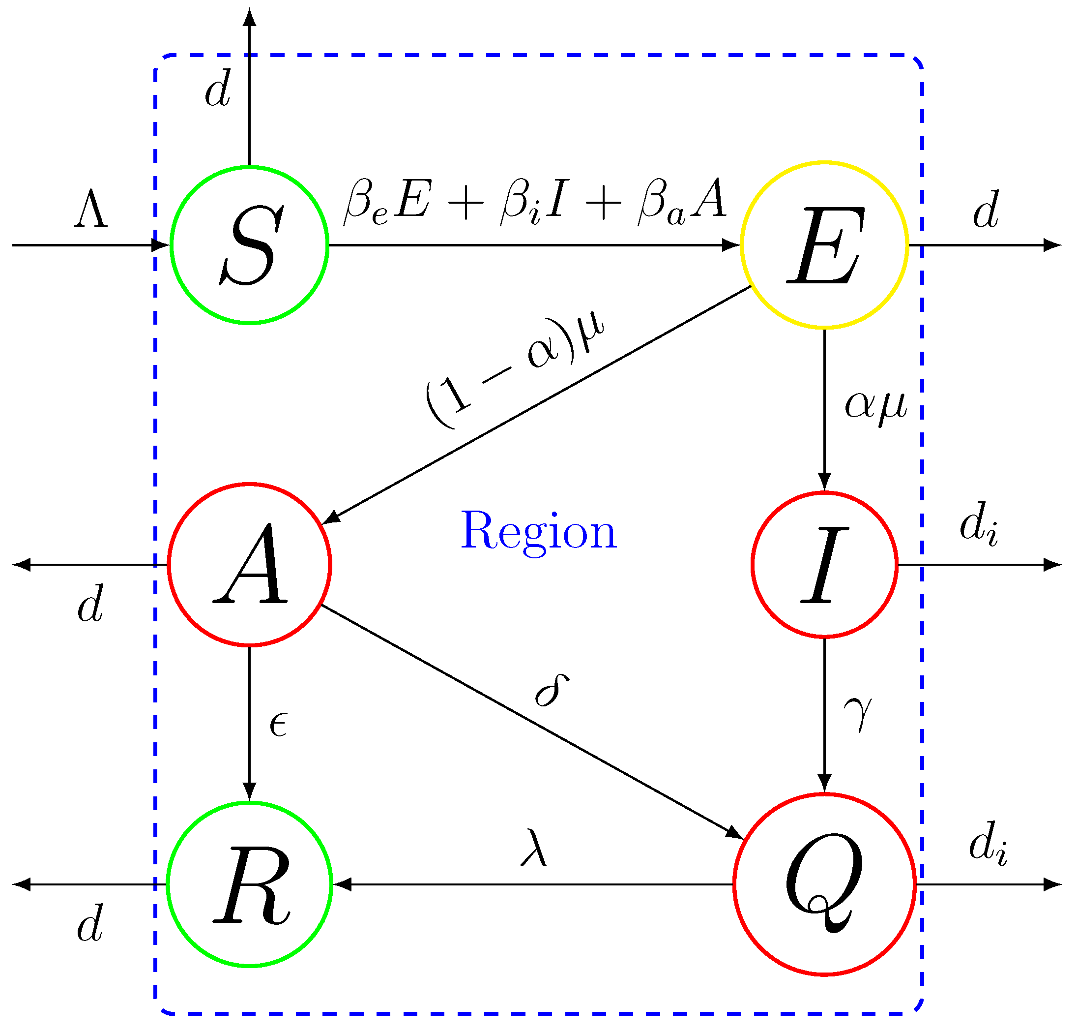
As described above, the SEIAQR compartmental model is presented to analyze the dynamic characteristics of the COVID-19 epidemic (Figure 1). It considers the asymptomatic infection, a transmissible incubation period. The isolation/quarantine is regarded as the major strategy to keep social distance. We establish the following six-dimensional differential equations to demonstrate the propagation dynamics of the transmission system:

$$\left\{\begin{array}{ccc}\hfill \dot{S}& =& \Lambda -{\beta }_{e}SE-{\beta }_{i}SI-{\beta }_{a}SA-dS,\hfill \\ \hfill \dot{E}& =& {\beta }_{e}SE+{\beta }_{i}SI+{\beta }_{a}SA-\mu E-dE,\hfill \\ \hfill \dot{I}& =& \alpha \mu E-\gamma I-d_{i}I,\hfill \\ \hfill \dot{A}& =& (1-\alpha )\mu E-\delta A-ϵA-dA,\hfill \\ \hfill \dot{Q}& =& \delta A+\gamma I-\lambda Q-d_{i}Q,\hfill \\ \hfill \dot{R}& =& ϵA+\lambda Q-dR.\hfill \end{array}\right.$$

(1)

where S, E, I, A, Q and R denote the susceptible, exposed (incubation period), infected, asymptomatic, documented confirmed (self-isolated or quarantined) and recovered individuals at time t, respectively. $\Lambda >0$ represents the influx individuals. ${\beta }_e>0$, ${\beta }_i>0$ and ${\beta }_a>0$ are infection rates of susceptible by close contacting the exposed, symptomatic infected and asymptomatic infected populations, respectively. $\frac{1}{\mu }$ is the average time of the exposed period. $\alpha$ represents the proportion of the symptomatic infected patients and $1-\alpha$ represents the asymptomatic ones. $\gamma >0$ is the confirmed portion of symptomatic infected cases and $\delta >0$ represents the confirmed portion of asymptomatic cases. $ϵ>0$ and $\lambda >0$ are the rates of transition from asymptomatic infections into recovered individuals, and from confirmed infections into recovered individuals, respectively. $d>0$ is the natural mortality rate. $d_i>0$ denotes the death rate of confirmed individuals which satisfies $0<d\le d_i$, as COVID-19 should result in excess deaths [55]. The population size of this system is varying and $d_i$ are considered in these variable-population-size models [56,57]. In our model, $d_i$ participates in the dynamics of the system by affecting the I compartment.

Figure 1. The flowchart of the SEIAQR model in a region.

There does not exist a negative solution for the system (1) with non-negative initial conditions (the infections can’t be negative).

Lemma 1.

The solution $(S,E,I,A,Q,R)$ of system (1) with the positive initial condition is positive and every forward solution $(S,E,I,A,Q,R)$ of system (1) eventually enters

$$\Omega =\left\{(S,E,I,A,Q,R)\in R_{+}^6:0\le S+E+I+A+Q+R\le \frac{\Lambda }{d}\right\}.$$

(2)

Then, Ω is a positively invariant set for system (1).

Proof. 

The solution $(S,E,I,A,Q,R)$ is assumed to available and be unique on $[0,T]$, where $T\le \infty$. Set

$$\hslash \left(t\right)={\beta }_{e}E+{\beta }_{i}I+{\beta }_{a}A.$$

(3)

Therefore, the first equation of system (1) can be expressed as

$$\dot{S}=\Lambda -\hslash \left(t\right)S-dS\ge -\hslash \left(t\right)S-dS,$$

(4)

we have

$${\displaystyle S\ge S\left(0\right)e^{-{\int }_0^t(\hslash \left(\sigma \right)+d)\mathrm{d}\sigma }>0,0\le t<T.}$$

(5)

Hence, $E\left(t\right)>0$ is hold for $0\le t<T$. Otherwise, there will exist a $t^{\prime }\in (0,T)$ satisfying $E\left(t^{\prime }\right)=0$ and $E\left(t\right)>0$ for $0<t<t^{\prime }$. Therefore,

$$\dot{I}=\alpha \mu E-\gamma I-d_{i}I\ge -\gamma I-d_{i}I,0<t<t^{\prime }$$

(6)

and

$$\dot{A}=(1-\alpha )\mu E-\delta A-ϵA-dA\ge -\delta A-ϵA-dA,0<t<t^{\prime }.$$

(7)

Integrating these two inequalities from 0 to t yields

$$I\ge I\left(0\right)e^{-(\gamma +d_i)t}>0$$

(8)

and

$$A\ge A\left(0\right)e^{-(\delta +ϵ+d)t}>0$$

(9)

for all $t\in (0,t^{\prime })$. Under the prerequisite $S>0$, $E>0$, $I>0$ and $A>0$ for all $t\in [0,t^{\prime }]$, the following inequalities are hold

$$\dot{E}={\beta }_{e}SE+{\beta }_{i}SI+{\beta }_{a}SA-\mu E-dE\ge -\mu E-dE,$$

(10)

and

$$E\left(t^{\prime }\right)\ge E\left(0\right)e^{-(\mu +d)t^{\prime }}>0,$$

(11)

which contradict to $E\left(t^{\prime }\right)=0$. Therefore, $E\left(t\right)>0$ for $0\le t<T$ is always hold. According to (8) and (9), $I>0$ and $A>0$ can be verified for all $t\in [0,T)$. By the last two equation of the system (1), we obtain

$$Q\ge Q\left(0\right)e^{-(\lambda +d_i)t}>0$$

(12)

and

$$R\ge R\left(0\right)e^{-dt}>0$$

(13)

for all $t\in [0,T)$. Hence, the solution of system (1) is positive with a positive initial condition.

Note that $N=S+E+I+A+Q+R$, where N represents overall populations at time t, and

$$\dot{N}=\Lambda -d(S+E+A+R)-d_i(I+Q)$$

(14)

The natural mortality rate is no greater than the COVID-19 death rate, i.e., $d\le d_i$, which leads to

$$\dot{N}\le \Lambda -d(S+E+A+R+I+Q)=\Lambda -dN.$$

(15)

When the epidemic is eradicated,

$$\underset{t\to \infty }{lim}N\left(t\right)=N_0=\frac{\Lambda }{d}.$$

(16)

As $N>N_0$, $\frac{\mathrm{d}N}{\mathrm{d}t}<0$, which implies that $\Omega$ is positively invariant with respect to system (1). Lemma 1 is proved. □

3. Equilibrium and Reproduction Number

First, all the derivatives in the system are set to zero in order to find the disease-free equilibrium (DFE). The following solution is achieved.

$$\dot{S}=\dot{E}=\dot{I}=\dot{A}=\dot{Q}=\dot{R}=0.$$

(17)

A DFE of the system (1) always exists at

$${\mathrm{E}}_0=\left(\frac{\Lambda }{d},0,0,0,0,0\right).$$

(18)

By the general calculation procedure of the basic reproduction number in [58], the new infection matrix $\mathcal{F}$ and the M-matrix, $\mathcal{V}$, of the transition terms are proposed as

$$\mathcal{F}=\left[\begin{array}{ccc}{\beta }_e{N}_0& {\beta }_i{N}_0& {\beta }_a{N}_0\\ 0& 0& 0\\ 0& 0& 0\end{array}\right]$$

(19)

and

$$\mathcal{V}=\left[\begin{array}{ccc}\mu +d& 0& 0\\ -\alpha \mu & \gamma +d_i& 0\\ -(1-\alpha )\mu & 0& \delta +ϵ+d\end{array}\right].$$

(20)

Then, the basic reproduction number of system (1) is obtained as the spectral radius of $\mathcal{F}{\mathcal{V}}^{-1}$ [58]. $R_0=\rho \left(\mathcal{F}{\mathcal{V}}^{-1}\right)$, i.e.,

$${\displaystyle R_0={\beta }_e\frac{\Lambda }{d(\mu +d)}+{\beta }_i\frac{\alpha \mu \Lambda }{d(\gamma +d_i)(\mu +d)}+{\beta }_a\frac{(1-\alpha )\mu \Lambda }{d(\delta +ϵ+d)(\mu +d)}}$$

(21)

and the effective reproduction number

$$R_t=\frac{S\left(t\right)}{N\left(t\right)}{R}_0,$$

(22)

which represent the transmission potential of the infectious disease. As can be seen, $R_0$ is composed of three parts comprising the transmission from the exposed, symptomatic infected and asymptomatic infected patients. It is more complex and accurate than other simplified models. When $R_0<1$, system (1) claims to have a unique DFE at ${\mathrm{E}}_0$. On the other hand, when $R_0⩾1$, the positive solution of (17) yields

$$\begin{array}{ccc}\hfill S^{*}& =& {\displaystyle \frac{\Lambda }{R_0-1},}\hfill \\ \hfill E^{*}& =& {\displaystyle \frac{\Lambda }{(\mu +d)R_0}(R_0-1),}\hfill \\ \hfill I^{*}& =& {\displaystyle \frac{\alpha \mu }{\gamma +d_i}\frac{\Lambda }{(\mu +d)R_0}(R_0-1),}\hfill \\ \hfill A^{*}& =& {\displaystyle \frac{(1-\alpha )\mu }{\delta +ϵ+d}\frac{\Lambda }{(\mu +d)R_0}(R_0-1),}\hfill \\ \hfill Q^{*}& =& {\displaystyle \frac{1}{\lambda +d_i}(\delta A^{*}+\gamma I^{*}),}\hfill \\ \hfill R^{*}& =& {\displaystyle \frac{1}{\lambda }(ϵA^{*}+\lambda Q^{*}).}\hfill \end{array}$$

(23)

Note that when $R_0=1$, system (1) reaches the DFE at ${\mathrm{E}}_0$. The system (1) reaches a unique endemic equilibrium (EE) at ${\mathrm{E}}^{*}=(S^{*},E^{*},I^{*},A^{*},Q^{*},R^{*})$ when $R_0>1$. Therefore, the system (1) has a unique DFE at ${\mathrm{E}}_0$ as $R_0⩽1$ and a unique EE at ${\mathrm{E}}^{*}$ as $R_0>1$. In the next section, we discuss both local and global asymptotically stability of the DFE and EE.

4. Stability Analysis of the DFE

First, we investigate the local stability of the DFE in the case $R_0⩽1$. The stability of higher-order complex systems is difficult to be determined by algebraic calculation. Thus, the following Lemma will be applied for discussing the local stability of DFE.

Lemma 2

([59]). A is stable if there exist positive definite matrix $P=P^T$ satisfying

$$PA+A^{T}P<0.$$

(24)

Theorem 1.

The DFE ${\mathrm{E}}_0$ of system (1) is locally asymptotically stable if only if $R_0<1$.

Proof. 

Since equations $\dot{Q}$ and $\dot{R}$ don’t interfere with the other equations, the sub-system composed of the first four equations in System (1) is linearized at equilibrium point ${\mathrm{E}}_0^{\prime }$. The Jacobian matrix $J\left({\mathrm{E}}_0^{\prime }\right)$ of the sub-system is

$$J\left({\mathrm{E}}_0^{\prime }\right)=\left[\begin{array}{cccc}-d& -{\beta }_e{S}_0& -{\beta }_i{S}_0& -{\beta }_a{S}_0\\ 0& {\beta }_e{S}_0-\mu -d& {\beta }_i{S}_0& {\beta }_a{S}_0\\ 0& \alpha \mu & -\gamma -d_i& 0\\ 0& (1-\alpha )\mu & 0& -\delta -ϵ-d\end{array}\right]$$

(25)

It is obvious that $J\left({\mathrm{E}}_0^{\prime }\right)$ has always one negative eigenvalue, ${\lambda }_1=-d$. The other eigenvalues of $J\left({\mathrm{E}}_0\right)$ should be achieved out of the following $3\times 3$ matrix

$$M=\left[\begin{array}{ccc}{\beta }_e{S}_0-\mu -d& {\beta }_i{S}_0& {\beta }_a{S}_0\\ \alpha \mu & -\gamma -d_i& 0\\ (1-\alpha )\mu & 0& -\delta -ϵ-d\end{array}\right]=\mathcal{F}-\mathcal{V}$$

(26)

where $\mathcal{F}$ and $\mathcal{V}$ are given in (19) and (20).

Set $\nu$ is the eigenvector of $\mathcal{V}$ with satisfying

$$\overline{\lambda }\nu =\mathcal{V}\nu$$

(27)

where $\overline{\lambda }>0$ is the eigenvalue of $\mathcal{V}$. Give following expression

$${\nu }^{T}PM\nu +{\nu }^T{M}^{T}P\nu ={\nu }^{T}P(\mathcal{F}{\mathcal{V}}^{-1}-I)\mathcal{V}\nu +{\nu }^T{\left({\mathcal{V}}^{-1}\right)}^T{(\mathcal{F}{\mathcal{V}}^{-1}-I)}^{T}P\nu$$

(28)

By Equation (27), we have

$${\nu }^{T}PM\nu +{\nu }^T{M}^{T}P\nu =\overline{\lambda }{\nu }^{T}P(\mathcal{F}{\mathcal{V}}^{-1}-I)\nu +\overline{\lambda }{\nu }^T{(\mathcal{F}{\mathcal{V}}^{-1}-I)}^{T}P\nu .$$

(29)

matrix $(\mathcal{F}{\mathcal{V}}^{-1}-I)$ is stable due to $R_0=\rho \left(\mathcal{F}{\mathcal{V}}^{-1}\right)<1$. Thus, there exists a positive definite matrix P subject to

$$PM+M^{T}P=\overline{\lambda }P(\mathcal{F}{\mathcal{V}}^{-1}-I)+\overline{\lambda }{(\mathcal{F}{\mathcal{V}}^{-1}-I)}^{T}P<0.$$

(30)

According to Lemma 2, the matrix M is stable.

Therefore, the system DFE is locally asymptotically stable if and only if $R_0<1$. □

Theorem 2.

The DFE ${\mathrm{E}}_0$ of system (1) is globally asymptotically stable if and only if $R_0⩽1$.

Proof. 

Since exposed individuals, symptomatic and asymptomatic infected patients are able to spread the COVID-19 disease. The Lyapunov function can be constructed by the variables $(E,I,A)$ to illustrate the dynamic characteristics of the DFE. Hence, the Lyapunov function is given by

$$V(E,I,A)=\frac{1}{\mu +d}\left({\beta }_e+\frac{{\beta }_i\alpha \mu }{\gamma +d_i}+\frac{{\beta }_a(1-\alpha )\mu }{\delta +ϵ+d}\right)E+\frac{{\beta }_i}{\gamma +d_i}I+\frac{{\beta }_a}{\delta +ϵ+d}A$$

(31)

Then, the total derivative of $V(E,I,A)$ is obtained with the following description.

$$\begin{array}{ccc}\hfill \dot{V}& =& \frac{1}{\mu +d}\left({\beta }_e+\frac{{\beta }_i\alpha \mu }{\gamma +d_i}+\frac{{\beta }_a(1-\alpha )\mu }{\delta +ϵ+d}\right)({\beta }_{e}SE+{\beta }_{i}SI+{\beta }_{a}SA)-({\beta }_{e}E+{\beta }_{i}I+{\beta }_{a}A)\hfill \\ \hfill & =& ({\beta }_{e}E+{\beta }_{i}I+{\beta }_{a}A)\left[{\displaystyle {\beta }_e\frac{1}{\mu +d}+{\beta }_i\frac{\alpha \mu }{(\gamma +d_i)(\mu +d)}+{\beta }_a\frac{(1-\alpha )\mu }{(\delta +ϵ+d)(\mu +d)}}\right]S\hfill \\ \hfill & & -({\beta }_{e}E+{\beta }_{i}I+{\beta }_{a}A)\hfill \\ \hfill & \le & ({\beta }_{e}E+{\beta }_{i}I+{\beta }_{a}A)(R_0-1)\le 0\hfill \end{array}$$

(32)

It is known that $\dot{V}=0$ holds if and only if $E=I=A=0$ or $R_0=1$. Obviously, the single point set $\left\{{\mathrm{E}}_0\right\}$ is a Maximum invariant set in $\left\{(S,E,I,A,Q,R)\in R_{+}^6|\dot{V}=0\right\}$. Therefore, the necessary and sufficient condition of globally asymptotically stability for the system’s DFE ${\mathrm{E}}_0$ is $R_0⩽1$. □

5. Stability Analysis of EE

Definition 1.

System (1) is said to be uniformly persistent if there exists a constant $0<c<\frac{\Lambda }{d}$ such that any solution $(S,E,I,A)$ with $(S\left(0\right),E\left(0\right),I\left(0\right),A\left(0\right))\in \mathring{\Omega }$ satisfies

$$min\{lim\underset{t\to \infty }{inf}S\left(t\right),lim\underset{t\to \infty }{inf}E\left(t\right),lim\underset{t\to \infty }{inf}I\left(t\right),lim\underset{t\to \infty }{inf}A\left(t\right)\}⩾c$$

(33)

where $\mathring{\Omega }$ denotes the interior of Ω [60].

Let X be a locally compact metric space with metric $\mathcal{D}$. Let $\Gamma$ be a closed nonempty subset of X with boundary $\partial \Gamma$ and interior $\mathring{\Gamma }$. Clearly, $\partial \Gamma$ is a closed subset of $\Gamma$. Let ${\Pi }_t$ be a dynamical system defined on $\Gamma$. Then, a set $\Delta$ in X is said to be invariant if $\Pi (\Delta ,t)=\Delta$. Define $M_{\partial }:=\{x\in \partial \Gamma :{\Pi }_{t}x\in \partial \Gamma ,\forall t⩾0\}$.

Lemma 3

([61,62]). Assume

A1. 

${\Pi }_t$ has a global attractor;

A2. 

There exists an $M=\{M_1,\cdots ,M_k\}$ of pair-wise disjoint, compact, and isolated invariant set on $\partial \Gamma$ such that

b1. 

${\cup }_{x\in M_{\partial }}\omega \left(x\right)\subset {\cup }_{j=1}^k{M}_j$;

b2. 

No subsets of M form a cycle on $\partial \Gamma$;

b3. 

Each $M_j$ is also isolated in Γ;

b4..

$W^s\left(M_j\right)\cap \Gamma =⌀$ for each $1⩽j⩽k$, where $W^s\left(M_j\right)$ is the stable manifold of $M_j$.

Then ${\Pi }_t$ is uniformly persistent with respect to Γ.

By applying Lemma 3, set $\Gamma =\Omega$, $\mathring{\Gamma }:=\{(S,E,I,A)\in \Gamma :E,I,A>0\}$ and $\partial \Gamma =\Gamma /\mathring{\Gamma }$. It is easy to verify that $M_{\partial }=\partial \Gamma$. On the boundary $\partial \Gamma$, system (1) reduce to

$$\dot{S}=\Lambda -dS.$$

(34)

Then

$$S\to \frac{\Lambda }{d},t\to \infty .$$

(35)

Obviously, $M=\left\{{\mathrm{E}}_0\right\}$ and $\omega \left(x\right)=\left\{{\mathrm{E}}_0\right\}$ for all $x\in M_{\partial }$, which implies that assumptions (b1) and (b2) hold. If $R_0>1$, the DFE is unstable from the Theorem 4 and we can obtain $W^s\left(M_j\right)=\partial \Gamma$, which means Assumptions (b3) and (b4) hold. The ultimate boundedness of all solutions to system (1) guarantees the existence of a global attractor making (A1) true. Therefore, the following Theorem 3 holds.

Theorem 3.

For system (1), the infectious disease will be extinct when $R_0⩽1$ and persistent when $R_0>1$.

Next, we will discuss the stability of EE in the case $R_0>1$, which can demonstrate the transmission dynamics in long term.

Theorem 4.

The endemic equilibrium ${\mathrm{E}}^{*}$ is locally asymptotically stable if $R_0>1$.

Proof. 

We introduce an auxiliary variable Y satisfying

$$S+E+I+A+Q+R+Y=\frac{\Lambda }{d},$$

(36)

then,

$$\dot{Y}=-\Lambda +d(S+E+A+R)+d_i(I+Q)$$

(37)

and

$$Y^{*}=\frac{\Lambda }{d}-S^{*}-E^{*}-I^{*}-A^{*}-Q^{*}-R^{*}.$$

(38)

We have $S=\frac{\Lambda }{d}-E-I-A-Q-R-Y$ from Equation (36). Substituting S into the first equation in system (1), we get the following system

$$\begin{array}{ccc}\hfill \dot{E}& =& {\beta }_{e}SE+{\beta }_{i}SI+{\beta }_{a}SA-\mu E-dE\hfill \\ \hfill \dot{I}& =& \alpha \mu E-\gamma I-d_{i}I\hfill \\ \hfill \dot{A}& =& (1-\alpha )\mu E-\delta A-ϵA-dA\hfill \\ \hfill \dot{Q}& =& \delta A+\gamma I-\lambda Q-d_{i}Q\hfill \\ \hfill \dot{R}& =& ϵA+\lambda Q-dR\hfill \\ \hfill \dot{Y}& =& -\Lambda +d(S+E+A+R)+d_i(I+Q)\hfill \end{array},$$

(39)

We will prove the local stability of the EE of system (1) when $R_0>1$ instead by system (39) by following the method given in [63,64], adopting the Krasnoselskii technique [65]. Consider the differential system

$$\dot{\overline{x}}=\psi \left(\overline{x}\right).$$

(40)

The local asymptotic stability of an equilibrium point ${\overline{x}}_0$ of the system (40) is equivalent to the linearized system

$$\dot{\overline{Z}}={\left.\frac{\mathrm{d}\psi \left(\overline{x}\right)}{\mathrm{d}\overline{x}}\right|}_{\overline{x}={\overline{x}}_0}\overline{Z}$$

(41)

has no solution of the form

$$\overline{Z}={\overline{Z}}_0{e}^{\omega t}$$

(42)

with ${\overline{Z}}_0\in C^n-\left\{0\right\},\omega \in C$ and $Re\omega ⩾0$, where $C^n$ is the n-dimensional complex coordinate space. By this method, the solution of EE of system (39) is substituted by the form (42). Then, the linear equations are obtained.

$$\begin{array}{ccc}\hfill \omega Z_1& =& \left[{\beta }_e(\frac{\Lambda }{d}-E^{*}-I^{*}-A^{*}-Q^{*}-R^{*}-Y^{*})-({\beta }_e{E}^{*}+{\beta }_i{I}^{*}+{\beta }_a{A}^{*})-(\mu +d)\right]Z_1\hfill \\ & & +\left[{\beta }_i(\frac{\Lambda }{d}-E^{*}-I^{*}-A^{*}-Q^{*}-R^{*}-Y^{*})-({\beta }_e{E}^{*}+{\beta }_i{I}^{*}+{\beta }_a{A}^{*})\right]Z_2\hfill \\ & & +\left[{\beta }_a(\frac{\Lambda }{d}-E^{*}-I^{*}-A^{*}-Q^{*}-R^{*}-Y^{*})-({\beta }_e{E}^{*}+{\beta }_i{I}^{*}+{\beta }_a{A}^{*})\right]Z_3\hfill \\ & & -({\beta }_e{E}^{*}+{\beta }_i{I}^{*}+{\beta }_a{A}^{*})Z_4-({\beta }_e{E}^{*}+{\beta }_i{I}^{*}+{\beta }_a{A}^{*})Z_5\hfill \\ & & -({\beta }_e{E}^{*}+{\beta }_i{I}^{*}+{\beta }_a{A}^{*})Z_6\hfill \\ \hfill \omega Z_2& =& \alpha \mu Z_1-(\gamma +d_i)Z_2\hfill \\ \hfill \omega Z_3& =& (1-\alpha )\mu Z_1-(\delta +ϵ+d)Z_3\hfill \\ \hfill \omega Z_4& =& \gamma Z_2+\delta Z_3-(\lambda +d_i)Z_4\hfill \\ \hfill \omega Z_5& =& ϵZ_3+\lambda Z_4-d{Z}_5\hfill \\ \hfill \omega Z_6& =& (d_i-d)Z_2+(d_i-d)Z_4-d{Z}_6\hfill \end{array}$$

(43)

where $Z_i\in C,i=1,\cdots ,6$, $E^{*}$, $I^{*}$,$A^{*}$,$Q^{*}$,$R^{*}$ and $Y^{*}$ are the coordinates of the endemic equilibrium of system (39). According to the system (17) and $R_t>1$, we define three variables and the following equations hold.

$$\begin{array}{ccc}\hfill \zeta & :=& {\displaystyle {\beta }_e(-\frac{\Lambda }{d}+E^{*}+I^{*}+A^{*}+Q^{*}+R^{*}+Y^{*})+({\beta }_e{E}^{*}+{\beta }_i{I}^{*}+{\beta }_a{A}^{*})+(\mu +d)}\hfill \\ \hfill & =& \left[{\displaystyle \frac{\alpha \mu {\beta }_i{N}_0}{(\gamma +d_i)R_0(R_0-1)}+\frac{(1-\alpha )\mu {\beta }_a{N}_0}{(\delta +ϵ+d)R_0(R_0-1)}+d}\right](R_0-1)>0\hfill \end{array},$$

(44)

$$\phi :=\frac{\Lambda }{d}-E^{*}-I^{*}-A^{*}-Q^{*}-R^{*}-Y^{*}=\frac{N_0}{R_0}>0$$

(45)

and

$$\rho :={\beta }_e{E}^{*}+{\beta }_i{I}^{*}+{\beta }_a{A}^{*}>0.$$

(46)

Then, solving the equations in (43) and making some manipulations, we can obtain

$$(1+G_i\left(\omega \right))Z_i={\left(HU\right)}_i,$$

(47)

where $U={(Z_1,Z_2,Z_3,Z_4,Z_5,Z_6)}^T$ and

$$G_1\left(\omega \right)=\frac{\omega +\rho ({\psi }_1+{\psi }_2+{\psi }_3+{\psi }_4+{\psi }_5)}{\varsigma },G_2\left(\omega \right)=\frac{\omega }{\gamma +d_i}.$$

(48)

$$G_3\left(\omega \right)=\frac{\omega }{\delta +ϵ+d},G_4\left(\omega \right)=\frac{\omega }{\lambda +d_i},G_5\left(\omega \right)=\frac{\omega }{d},G_6\left(\omega \right)=\frac{\omega }{d}$$

(49)

and H is the matrix

$$H:=\left[\begin{array}{cccccc}0& {\beta }_i\phi & {\beta }_a\phi & 0& 0& 0\\ {\displaystyle \frac{\alpha \mu }{\gamma +d_i}}& 0& 0& 0& 0& 0\\ {\displaystyle \frac{(1-\alpha )\mu }{\delta +ϵ+d}}& 0& 0& 0& 0& 0\\ 0& {\displaystyle \frac{\gamma }{\lambda +d_i}}& {\displaystyle \frac{\delta }{\lambda +d_i}}& 0& 0& 0\\ 0& 0& {\displaystyle \frac{ϵ}{d}}& {\displaystyle \frac{\lambda }{d}}& 0& 0\\ 0& {\displaystyle \frac{d_i-d}{d}}& 0& {\displaystyle \frac{d_i-d}{d}}& 0& 0\end{array}\right]$$

(50)

where

$${\psi }_1:=\frac{\alpha \mu }{\gamma +d_i+\omega },{\psi }_2:=\frac{(1-\alpha )\mu }{\delta +ϵ+d+\omega },$$

$${\displaystyle {\psi }_3:=\frac{\gamma }{\lambda +d_i+\omega }\frac{\alpha \mu }{\gamma +d_i}+\frac{\delta }{\lambda +d_i+\omega }\frac{(1-\alpha )\mu }{\delta +ϵ+d+\omega },}$$

$${\displaystyle {\psi }_4:=\frac{ϵ}{d+\omega }\frac{(1-\alpha )\mu }{\delta +ϵ+d+\omega }+\frac{\lambda }{d+\omega }\left({\displaystyle \frac{\gamma }{\lambda +d_i+\omega }\frac{\alpha \mu }{\gamma +d_i}+\frac{\delta }{\lambda +d_i+\omega }\frac{(1-\alpha )\mu }{\delta +ϵ+d+\omega }}\right)}$$

and

$${\displaystyle {\psi }_5:=\frac{d_i-d}{d+\omega }\frac{\alpha \mu }{\gamma +d_i}+\frac{d_i-d}{d+\omega }\left({\displaystyle \frac{\gamma }{\lambda +d_i+\omega }\frac{\alpha \mu }{\gamma +d_i}+\frac{\delta }{\lambda +d_i+\omega }\frac{(1-\alpha )\mu }{\delta +ϵ+d+\omega }}\right)}$$

Obviously, the elements of H are non-negative. ${\overline{X}}^{*}=(E^{*},I^{*},A^{*},D^{*},R^{*},Y^{*})$ satisfies

$${\overline{X}}^{*}=H{\overline{X}}^{*}$$

(51)

Further, on condition that the positive coordinates of ${\overline{X}}^{*}$, if ${\overline{X}}^{*}$ is a solution of (47), there must be a minimal positive s which depends on $\overline{Z}$ satisfying

$$|\overline{Z}|\le s{\overline{X}}^{*}$$

(52)

where $|·|$ is the norm in C.

Further, to verify that $Re\omega <0$, we discuss two different scenarios: $\omega =0$ and $\omega \ne 0$. If $\omega =0$, the determinant of system (47) can be derived as

$$\Delta =1+G_1\left(0\right)>0.$$

(53)

Thus, the system (47) has only a trivial solution implying $\omega \ne 0$.

In the other scenario, we assume that $\omega \ne 0$ and $Re\omega ⩾0$. Let

$$G\left(\omega \right)=min\left\{|1+G_i\left(\omega \right)|,i=1,\cdots ,6\right\}.$$

(54)

It can be determined that $|1+G_i\left(\omega \right)|>1$ for any i. Thus, $G\left(\omega \right)>1$. We calculate the norms of (47). Considering H is non-negative, it can be achieved:

$$G\left(\omega \right)|\overline{Z}|⩽H|\overline{Z}|.$$

(55)

Combining (51) and (52) yields

$$G\left(\omega \right)|\overline{Z}|⩽sH{\overline{X}}^{*}=s{\overline{X}}^{*},$$

(56)

which implies

$$|\overline{Z}|⩽\frac{s{\overline{X}}^{*}}{G\left(\omega \right)}<s{\overline{X}}^{*}.$$

(57)

The result is contradicting the minimality of s. Hence, $Re\omega$ is negative. Above theorem is proved. □

Theorem 5.

The endemic equilibrium ${\mathrm{E}}^{*}$ is globally asymptotically stable if $R_0>1$.

Proof. 

We let

$$V\left(\varsigma \right)={\int }_{{\varsigma }^{*}}^{\varsigma }\frac{\tau -\varsigma }{\tau }\mathrm{d}\tau ,\varsigma >0$$

(58)

where ${\varsigma }^{*}>0$. Clearly, $V\left(\varsigma \right)⩾0$ with the equality holding if and only if $\varsigma ={\varsigma }^{*}$. $V\left(\varsigma \right)$ is applied to prove the globally asymptotically stability by replaced S, E, I or A. Differentiating the four functions $V\left(S\right)$, $V\left(E\right)$, $V\left(I\right)$ and $V\left(A\right)$ along the solution of system (1) and using the inequality $1-x+lnx⩽0$ for $x>0$ with equality holding if and only if $x=1$ yield

$$\begin{array}{ccc}\hfill \dot{V}\left(S\right)& =& {\displaystyle \frac{S-S^{*}}{S}\left({\beta }_e{S}^{*}{E}^{*}+{\beta }_i{S}^{*}{I}^{*}+{\beta }_a{S}^{*}{A}^{*}+d{S}^{*}-{\beta }_{e}SE-{\beta }_{i}SI-{\beta }_{a}SA-dS\right)}\hfill \\ \hfill & =& {\displaystyle -\frac{d{(S-S^{*})}^2}{S}+{\beta }_e{S}^{*}{E}^{*}\left({\displaystyle 1-\frac{S^{*}}{S}+\frac{E}{E^{*}}-\frac{SE}{S^{*}{E}^{*}}}\right)}\hfill \\ \hfill & & +{\beta }_i{S}^{*}{I}^{*}\left({\displaystyle 1-\frac{S^{*}}{S}+\frac{I}{I^{*}}-\frac{SI}{S^{*}{I}^{*}}}\right)+{\beta }_a{S}^{*}{A}^{*}\left({\displaystyle 1-\frac{S^{*}}{S}+\frac{A}{A^{*}}-\frac{SA}{S^{*}{A}^{*}}}\right)\hfill \end{array}$$

(59)

$$\begin{array}{ccc}\hfill \dot{V}\left(E\right)& =& {\displaystyle \frac{E-E^{*}}{E}\left({\beta }_{e}SE+{\beta }_{i}SI+{\beta }_{a}SA-\mu E-dE\right)}\hfill \\ \hfill & =& {\beta }_e{S}^{*}{E}^{*}\left({\displaystyle 1+\frac{SE}{S^{*}{E}^{*}}-\frac{E}{E^{*}}-\frac{S}{S^{*}}}\right)+{\beta }_i{S}^{*}{I}^{*}\left({\displaystyle 1+\frac{SI}{S^{*}{I}^{*}}-\frac{E}{E^{*}}-\frac{SI{E}^{*}}{S^{*}{I}^{*}E}}\right)\hfill \\ \hfill & & +{\beta }_a{S}^{*}{A}^{*}\left({\displaystyle 1+\frac{SA}{S^{*}{A}^{*}}-\frac{E}{E^{*}}-\frac{SA{E}^{*}}{S^{*}{A}^{*}E}}\right)\hfill \end{array}$$

(60)

Hence,

$$\begin{array}{ccc}\hfill \dot{V}\left(S\right)+\dot{V}\left(E\right)& ⩽& {\beta }_e{S}^{*}{E}^{*}\left({\displaystyle 2-\frac{S}{S^{*}}-\frac{S^{*}}{S}}\right)+{\beta }_i{S}^{*}{I}^{*}\left({\displaystyle 2-\frac{S^{*}}{S}+\frac{I}{I^{*}}-\frac{E}{E^{*}}}\right.\hfill \\ \hfill & & \left.{\displaystyle -\frac{SI{E}^{*}}{S^{*}{I}^{*}E}}\right)+{\beta }_a{S}^{*}{A}^{*}\left({\displaystyle 2-\frac{S^{*}}{S}+\frac{A}{A^{*}}-\frac{E}{E^{*}}-\frac{SA{E}^{*}}{S^{*}{A}^{*}E}}\right)\hfill \\ \hfill & ⩽& {\beta }_i{S}^{*}{I}^{*}\left({\displaystyle \frac{I}{I^{*}}-ln\frac{I}{I^{*}}+ln\frac{E}{E^{*}}-\frac{E}{E*}}\right)\hfill \\ \hfill & & +{\beta }_a{S}^{*}{A}^{*}\left({\displaystyle \frac{A}{A^{*}}-ln\frac{A}{A^{*}}+ln\frac{E}{E^{*}}-\frac{E}{E*}}\right)\hfill \end{array}$$

(61)

Similarly, one can verify that

$$\begin{array}{ccc}\hfill \dot{V}\left(I\right)& =& {\displaystyle \frac{I-I^{*}}{I}\left(\alpha \mu E-\gamma I-d_{i}I\right)}\hfill \\ \hfill & =& {\displaystyle \frac{I-I^{*}}{I}\left(\alpha \mu E-\alpha \mu E^{*}\frac{I}{I^{*}}\right)}\hfill \\ \hfill & =& \alpha \mu E^{*}\left({\displaystyle 1+\frac{E}{E^{*}}-\frac{I}{I^{*}}-\frac{I^{*}E}{I{E}^{*}}}\right)\hfill \\ \hfill & ⩽& \alpha \mu E^{*}\left({\displaystyle \frac{E}{E^{*}}-ln\frac{E}{E^{*}}+ln\frac{I}{I^{*}}-\frac{I}{I^{*}}}\right)\hfill \end{array}$$

(62)

and

$$\begin{array}{ccc}\hfill \dot{V}\left(A\right)& =& {\displaystyle \frac{A-A^{*}}{A}\left[\xi \mu E-\delta A-ϵA-dA\right]}\hfill \\ \hfill & =& {\displaystyle \frac{A-A^{*}}{A}\left[\xi \mu E-(1-\alpha )\mu E^{*}\frac{A}{A^{*}}\right]}\hfill \\ \hfill & =& \xi \mu E^{*}\left({\displaystyle 1+\frac{E}{E^{*}}-\frac{A}{A^{*}}-\frac{A^{*}E}{A{E}^{*}}}\right)\hfill \\ \hfill & ⩽& \xi \mu E^{*}\left({\displaystyle \frac{E}{E^{*}}-ln\frac{E}{E^{*}}+ln\frac{A}{A^{*}}-\frac{A}{A^{*}}}\right),\hfill \end{array}$$

(63)

where $\xi =1-\alpha$. Furthermore, we choose that

$${\displaystyle \mathcal{V}=V\left(S\right)+V\left(E\right)+\frac{{\beta }_i{S}^{*}{I}^{*}}{\alpha \mu E^{*}}V\left(I\right)+\frac{{\beta }_a{S}^{*}{A}^{*}}{\xi \mu E^{*}}V\left(A\right)}$$

(64)

as a Lyapunov function for system (1). Clearly, $\mathcal{V}⩾0$ and

$$\dot{\mathcal{V}}⩽0$$

(65)

with the equality holding if and only if $(S,E,I,A)=(S^{*},E^{*},I^{*},A^{*})$. And it is easily to verify that the single point set $\left\{(S^{*},E^{*},I^{*},A^{*})\right\}$ where $\mathcal{V}=0$ hold is the maximum invariant set. Thus, the globally asymptotically stability of the EE in $\Omega$ is proved. □

6. Sensitivity Analysis

6.1. Sensitivity Analysis of $R_0$

To optimize effective COVID-19 containment measures, it is critical to determine the relative influence of the different factors on transmission and prevalence. In this section, we carried out the sensitivity analysis to quantitatively evaluate the impact of transmission parameters from different compartments (E, I and A) and confirmation rates ($\gamma$ and $\delta$) on the reproduction number and equilibrium. The definition of elasticity is given by the percentage change in $R_0$ with respect to the percentage change in the infection or confirmation rates. And the sensitivity or elasticity is proposed by [66] as

$${\epsilon }_{R_0}^p=\frac{\partial R_0}{\partial p}/\frac{R_0}{p}=\frac{p}{R_0}\frac{\partial R_0}{\partial p}.$$

(66)

By applying the Equation (66) into the reproduction number $R_t$ which takes the form of (21), we have

$${\epsilon }_{R_0}^{\Lambda }=1.$$

(67)

According to the epidemic characteristics of COVID-19, $\mu \gg d$, $\gamma \gg d_i$ and $\delta +\epsilon \gg d$.

$${\displaystyle R_0\approx {\beta }_e\frac{\Lambda }{d\mu }+{\beta }_i\frac{\alpha \Lambda }{d\gamma }+{\beta }_a\frac{(1-\alpha )\Lambda }{d(\delta +ϵ)}}$$

(68)

Then, we have the sensitivity descriptions as

$${\epsilon }_{R_0}^d\approx -1$$

(69)

$${\displaystyle {\epsilon }_{R_0}^{{\beta }_e}\approx {\beta }_e\frac{\Lambda }{d\mu }\frac{1}{R_0}<1}$$

(70)

$${\displaystyle {\epsilon }_{R_0}^{{\beta }_i}\approx {\beta }_i\frac{\alpha \Lambda }{d\gamma }\frac{1}{R_0}<1}$$

(71)

$${\displaystyle {\epsilon }_{R_0}^{{\beta }_a}\approx {\beta }_a\frac{(1-\alpha )\Lambda }{d(\delta +ϵ)}\frac{1}{R_0}<1}$$

(72)

$${\displaystyle {\epsilon }_{R_0}^{\mu }\approx -{\beta }_e\frac{\Lambda }{d\mu }\frac{1}{R_0}}$$

(73)

$${\displaystyle {\epsilon }_{R_0}^{\gamma }\approx -{\beta }_i\frac{\alpha \Lambda }{d\gamma }\frac{1}{R_0}}$$

(74)

and

$${\displaystyle {\epsilon }_{R_0}^{\delta }\approx -{\beta }_a\frac{(1-\alpha )\Lambda }{d(\delta +ϵ)}\frac{1}{R_0}}$$

(75)

The number of ${\epsilon }_{R_0}^p$ represent that $1\%$ increase in each parameter p will result in ${\epsilon }_{R_0}^p\%$ increase in $R_0$. For instance, the reproduction number $R_0$ will increase or decrease by $1\%$ corresponding to $1\%$ increase $\Lambda$ and d ((67) and (69)).

6.2. Sensitivity Analysis of EE

Except for the reproduction number, sensitivity analysis is also performed for the EE point in this subsection. When the reproduction number is unable to be controlled to less than 1 (which is the common case all over the world), the disease will remain endemic as proved previously. The EE point $E^{*}=(S^{*},E^{*},I^{*},A^{*},Q^{*},R^{*})$ is directly related to the severity of COVID-19 transmission, $I^{*}$ in particular. The sensitivity analysis of EE should evaluate the significance of model parameters for endemic disease prevalence. Therefore, to determine the optimal strategy to minimize infected cases, several tests are carried out thus the parameters are selected that play a significant influence on the dynamics of the system. Few studies used similar methods to find the important input parameter for the EE point [52]. To simplify the expression for the sensitivity function, the EE point $(S^{*},E^{*},I^{*},A^{*},Q^{*},R^{*})$ has been replaced by $(u_1,u_2,u_3,u_4,u_5,u_6)$ and the parameters $(\Lambda ,d,{\beta }_a,{\beta }_e,{\beta }_i,\mu ,\gamma ,\delta )$ have been replaced by $(v_1,v_2,v_3,v_4,v_5,v_6,v_7,v_8)$. Then, the sensitivity indices of the EE point, $u_i$, to the system parameter, $v_j$ is given by

$${\epsilon }_{u_i^{*}}^{v_j}=\frac{\partial u_i^{*}}{\partial v_j}·\frac{v_j}{u_i^{*}},i=1,\cdots ,6,j=1,\cdots ,8.$$

(76)

7. Application of the Model

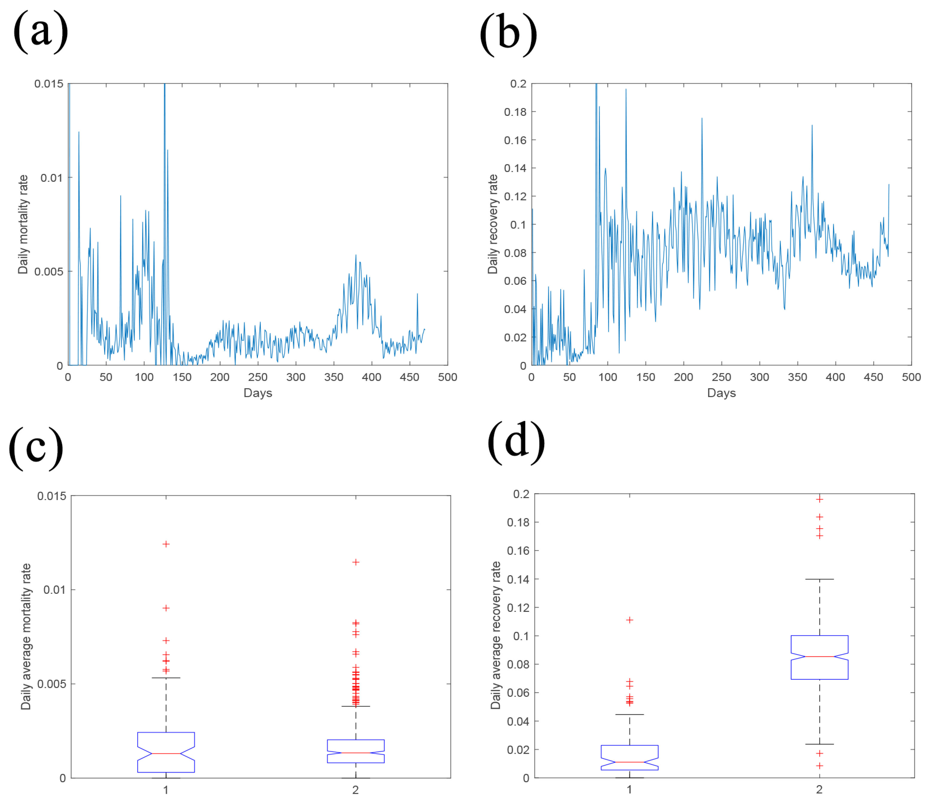
Further, to optimize the containment strategy and understand the COVID-19 transmission dynamics, we apply the model associated with analysis methods using the Japanese COVID-19 data from 27 March 2020 to 1 August 2020 as a realistic case exploration. The period is divided into three different stages according to the varied policies enforced by the government. Stage 1 is from 27 March to 6 April; stage 2 is from 7 April to 25 May (rigorous infection control measures with “declaration of a state of emergency”); stage 3 is from 26 May to 1 August (lifting of the state of emergency). The basic reproduction number $R_0$ is adopted in a stage without containment strategies and the effective reproduction number $R_t$ changes due to the different control strategies in stage 2 and stage 3. The model parameter $d=3.0\times {10}^{-5}$ and $\Lambda =2391$ are estimated by [67], $\mu =0.2$ [68] and $ϵ=0.0714$ [69]. The fatality rate due to COVID-19 is estimated as $0.0013$ based on the real data [70] as shown in Figure 2.

Figure 2. Determination of mortality and recovery rate. (a) Daily mortality rate; (b) Daily mortality rate; (c) Daily average mortality rate. (d) Daily average recovery rate. The first average mortality and recovery rate are statistically averaged over the period of stage 1, the second mortality rate is averaged over the period data of stage 2 and stage 3.

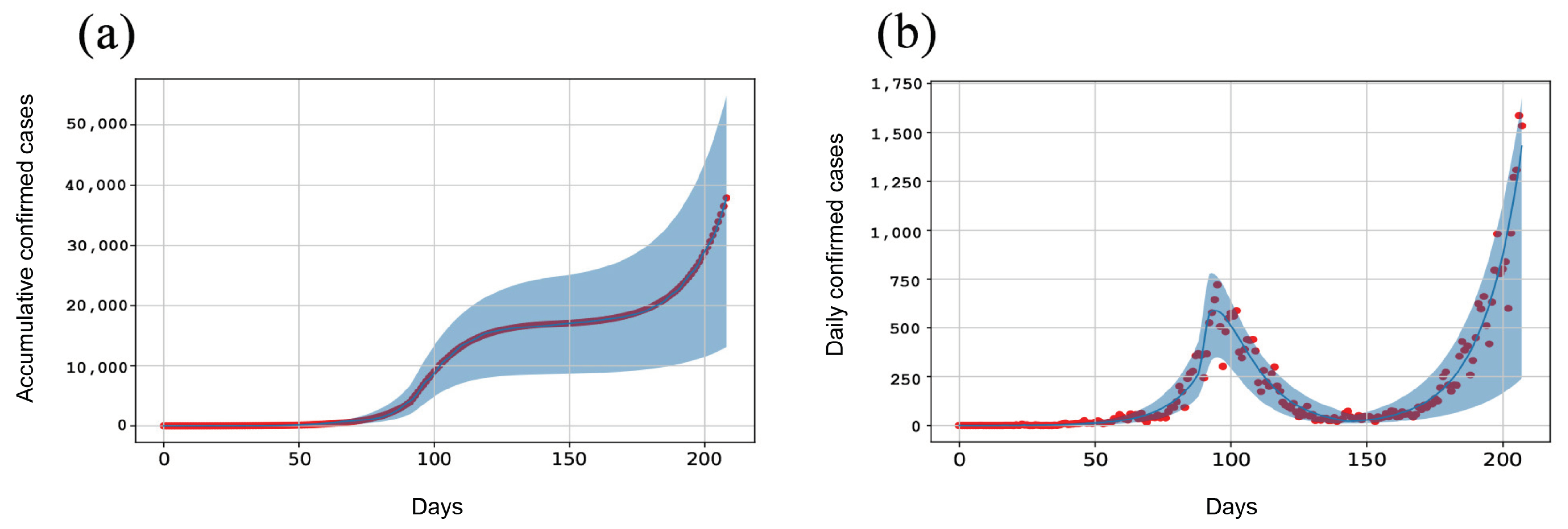
The parameters in the system ${\beta }_e$, ${\beta }_i$, ${\beta }_a$, $\delta$, $\gamma$, $\alpha$ are collected by fitting using the least square method. The fitting of cumulative cases is demonstrated in Figure 3a. The goodness of fitting [71] are 0.926 in stage 1; 0.939 in stage 2 and 0.939 in stage 3. The model parameters were determined by the least-square method. The confidential interval of cumulative infected cases was estimated in the following procedure (similar approach in a previous study [72]): (1) The initial simulated daily cases ID(t) are fitted with real Poisson noises on ID(t), we achieve the numerical daily infected cases ND(t). Then, the numerical cumulative cases NC(t) are determined by taking the sum of ND(t). (2) The least sum of squares of the difference between IC(t) and NC(t) are calculated and model parameters are estimated. (3) Using the estimated parameters, cumulative and daily cases are calculated. (4) The processes (1)–(3) are repeated 1000 times to achieve a range of simulated data. $95\%$ of the simulated data range are set as the confidential interval for Figure 3a,b. The parameters collected by fitting in the three stages are listed in Table 1. The outbreak and the spread of the epidemic are random events. A model characterized by stochastic differential equations (SDE) describes the COVID-19 transmission process more accurately than the ODE system. A better fitting by SDE model is expected with the cumulative or daily infected cases. The deterministic ODE system is established based on the assumption that the population size is large enough and the population is homogenous. It is relatively convenient to analyze the significance of asymptomatic infection in the COVID-19 development. Also, in the next section, a simple sensitivity analysis is adopted to analyze the prevention and control strategies for incubation period infection, symptomatic infection, and asymptomatic infection specifically. In order to understand the impact of the containment strategies, the investigation based on the ODE model is effective. It could be more difficult to conduct similar work for this point using the SDE model. Numerical methods should be used. To better implement strategies seeking a balance between economic development and epidemic prevention and control, it is more important to study SDE models. We will modify our model in the future work.

Figure 3. Application of the model with Japanese data. The duration of COVID-19 infection is separated into three stages. Stage 1 is the initial transmission period. Stage 2 is the period with highly restrictive measures in the state of emergency. Stage 3 is the period when the state of emergency is lifted. (a) Fitting of the cumulative infected cases. (b) Fitting of the daily infected cases. The red dots represent the real data points. The blue areas represent the confidential interval simulated by the model.

Table 1. Model parameters by fitting.

Parameters	Stage 1	Stage 2	Stage 3
${\beta }_e$	$0.0663$	$0.0001$	$0.0713$
${\beta }_i$	$0.1804$	$0.0006$	$0.1499$
${\beta }_a$	$0.2665$	$0.019$	$0.2335$
$\alpha$	$0.1092$	$0.5554$	$0.1205$
$\gamma$	$0.7373$	$0.16468$	$0.1323$
$\delta$	$0.0595$	$0.1372$	$0.0721$
$R_t$	$2.1014$	$0.3824$	$1.8004$

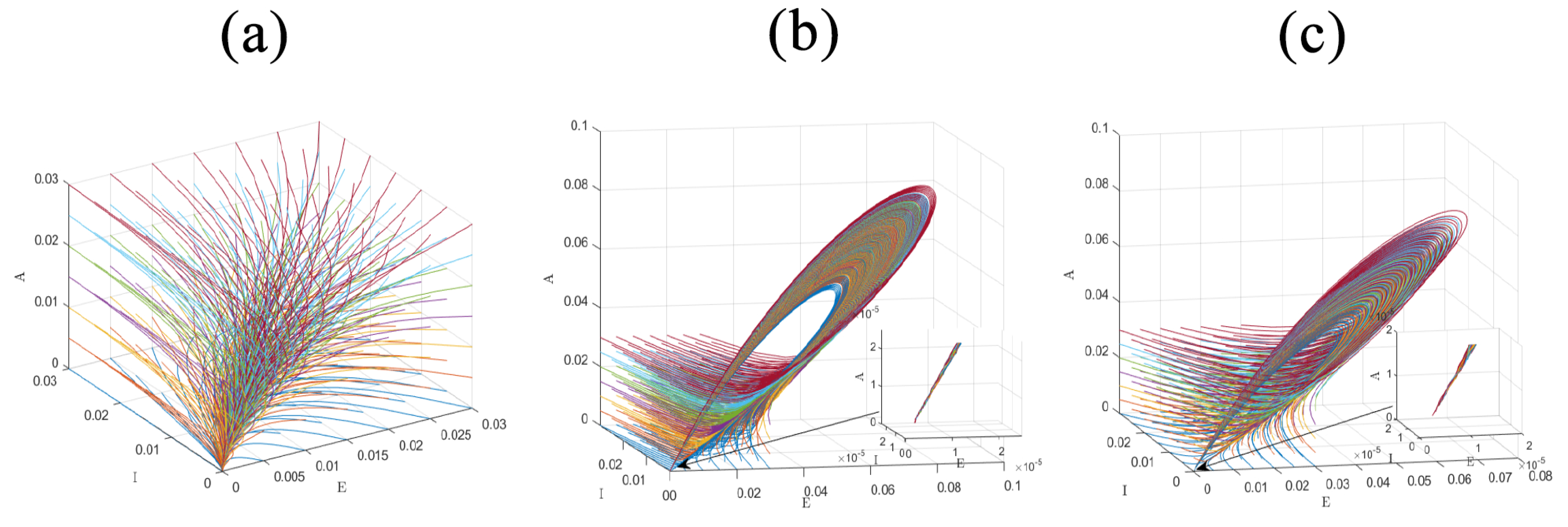
As we proved in the Section 4, COVID-19 will be eradicated with $R_0<1$. We simulate the development of the point $(E,I,A)$, the number of exposed, infected, and asymptomatic cases with $R_0<1$ (Figure 4a). The simulation adopts $R_0$ in stage 2 when a state of emergency is declared. At every initial conditions, $(E,I,A)$ will converge to $(0,0,0)$. The pandemic will reach an endemic equilibrium as Figure 4b shows the convergence point of $(E,I,A)$ with $R_0>1$. The simulation in Figure 4b uses $R_0$ in stage 1 with a weak control strategy. Figure 4c demonstrates the converging point with $R_0>1$ in stage 3 after the lifting of the stringent control policy. The highest number of infected cases can be affected by the starting point either for $R_0<1$ or $R_0>1$. The peak infections, if without control, can reach nearly 10% of the population at a single day with $R_0>1$ (upper right), which will bring tremendous burden to the healthcare system. Thus, even the disease free equilibrium cannot be achieved ($R_0>1$), the asymptomatic transmission rate must be reduced to avoid large portion of infections.

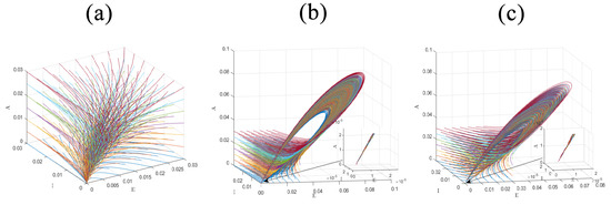
Figure 4. Three-dimensional phase portrait of $(E,I,A)$ trends. (a) All $(E,I,A)$ lines starting from different initial conditions approach to the origin with $R_t=0.3824$ (stage 2) which illustrate the vanish of COVID-19. (b) The $(E,I,A)$ lines reach a non-zero point which demonstrate the endemic equilibrium with $R_0=2.1014$ (stage 1). (c) The $(E,I,A)$ lines reach another non-zero point which demonstrate endemic equilibrium with $R_t=1.8004$ (stage 3).

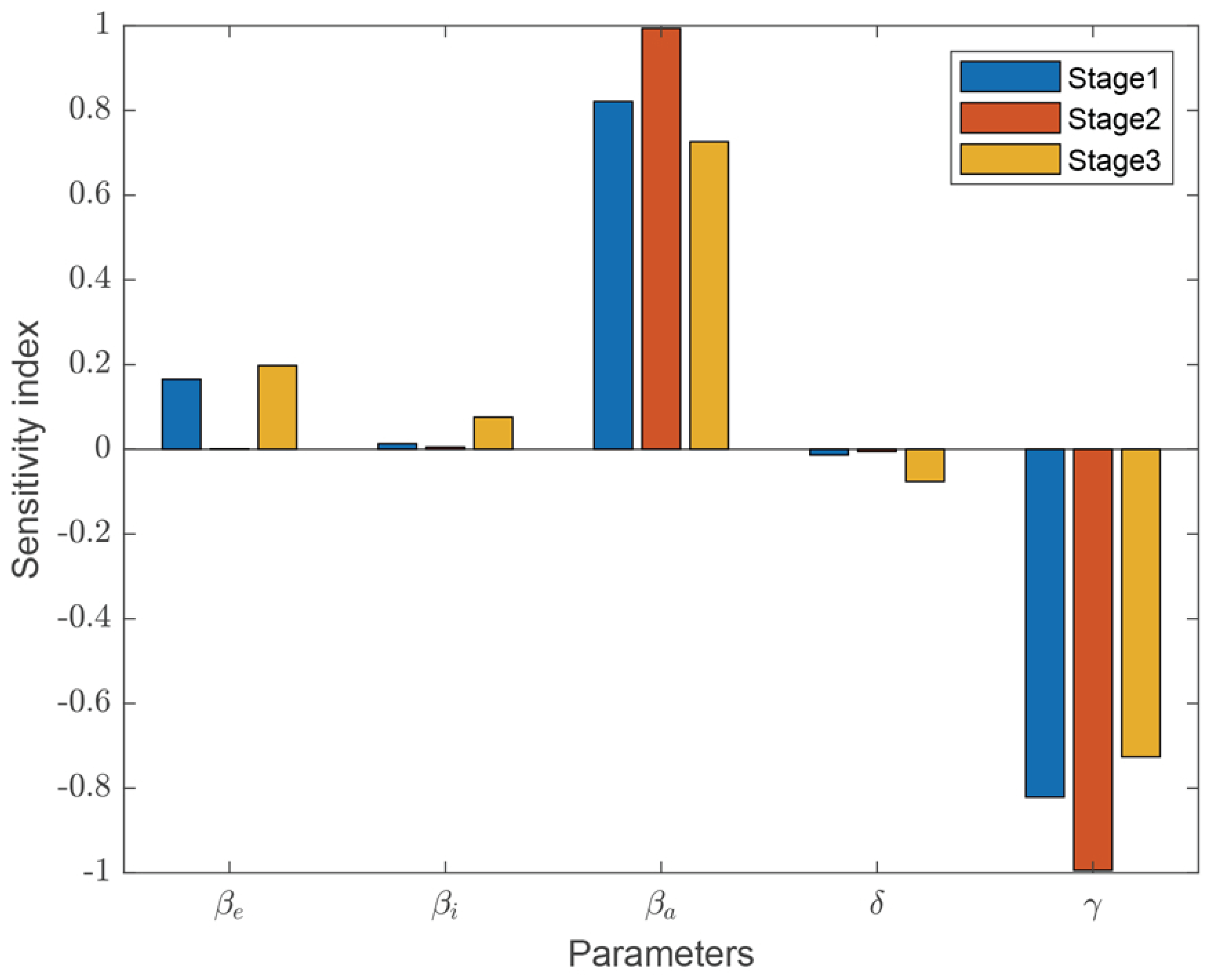
7.1. Sensitivity Analysis of $R_0$ to the Parameters

The sensitivity analysis of $R_0$ in response to the variation of model parameters are preformed for the three different stages (Figure 5). As can be seen in Table 2, the sensitivity indices ${\epsilon }_{R_0}^{{\beta }_a}$ (0.821 in stage 1, 0.994 in stage 2 and 0.726 in stage 3) are higher than the indices ${\epsilon }_{R_0}^{{\beta }_i}$ (0.166, 0.001 and 0.198, respectively) and ${\epsilon }_{R_0}^{{\beta }_e}$.

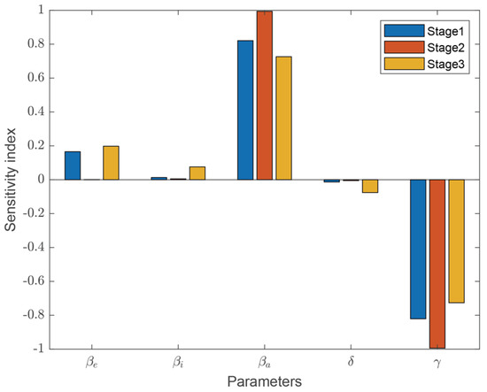
Figure 5. The sensitive indices determined with realistic data. Sensitivity indices of $R_0$ to the model parameters in the three stages.

Table 2. Sensitivity indices of $R_0$ in response to the variation of model parameters using reported data in three stages.

Parameters	Stage 1	Stage 2	Stage 3
${\beta }_e$	$0.01652$	$0.00078$	$0.19788$
${\beta }_i$	$0.01335$	$0.00520$	$0.07596$
${\beta }_a$	$0.82103$	$0.99402$	$0.72622$
$\gamma$	$-0.01335$	$-0.00520$	$-0.07590$
$\delta$	$-0.82103$	$-0.99402$	$-0.72622$

In this model, ${\beta }_i$ represents the transmission rate of the infected compartment. ${\beta }_e$ represents the transmission rate of the exposed compartment. ${\beta }_a$ represents the transmission rate of the asymptomatic compartment. Thus, controlling the asymptomatic transmission rates should be more effective in reducing $R_0$ [53]. $\delta$ and $\gamma$ represent the confirmation rate of the symptomatic and asymptomatic infected cases by testing. During the state of emergency (stage 2), it can be found that the ${\epsilon }_{R_0}^{\delta }$ which corresponds to the control of the infected cases is greatly reduced. But the sensitivity indices related to the asymptomatic transmission and the confirmation of the asymptomatic cases increased. Hence, even during the period when intensive restrictions are imposed, it is still of high importance to precisely control the asymptomatic cases.

7.2. Sensitivity Analysis of EE to the Parameters

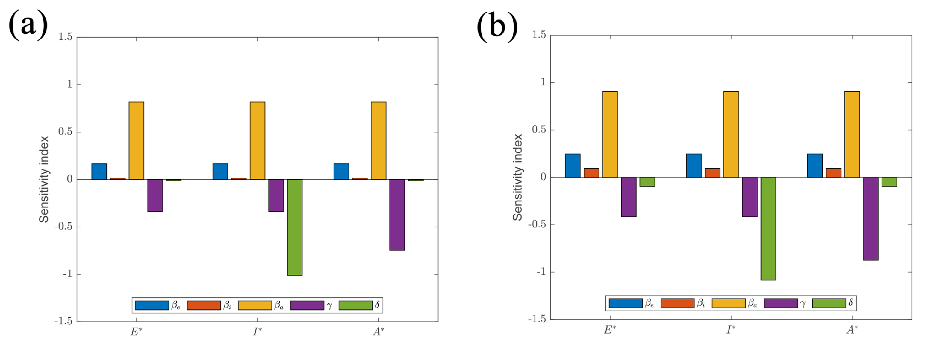
In stage 1 and stage 3 (before and after the state of emergency), $R_0$ and $R_t$ are greater than 1. The sensitivity indices of the EE point $(E,I,A)$ with respect to the model parameters are determined (as can be seen in Table 3 and a graphical illustration Figure 6). The relative significance of these parameters can also be determined to the endemic point (the expected overall cases represent the severity of the pandemic). In stage 1 and stage 3, it can be seen that positive sensitive parameters are transmission rates ${\beta }_i$, ${\beta }_e$, ${\beta }_a$. Reducing these transmission rates by control policies can decrease the total number of cases. Among the three different transmission rates, the sensitive parameter associated with ${\beta }_a$ is larger than ${\beta }_i$, ${\beta }_e$ for the EE point $(E,I,A)$. The negative sensitive parameters are confirmation rate $\delta$ and $\gamma$ (confirmation rate of the infected and asymptomatic cases). Reducing $\delta$ and $\gamma$ should increase the final infected number at the endemic equilibrium. It can be found that sensitive indices for E, A to $\gamma$ are larger than sensitive indices for E, A to $\delta$. Also, the sensitive indices for I to gamma are relatively large. Thus, the controlling the asymptomatic transmission and detecting the asymptomatic cases are of great influence in contributing to the severity of the COVID-19 endemic equilibrium. To decrease the final number of infections, the asymptomatic cases must be precisely determined.

Table 3. Sensitivity indices of endemic equilibrium $(E,I,A)$ in response to the model parameters in three stages.

Stage 1	E	I	A
${\beta }_e$	$0.16536$	$0.16536$	$0.16536$
${\beta }_i$	$0.01332$	$0.01332$	$0.01332$
${\beta }_a$	$0.81919$	$0.81919$	$0.81919$
$\gamma$	−0.33744	−0.33744	−0.74865
$\delta$	−0.01332	−1.01055	−0.01332
Stage 3	$\mathit{E}$	$\mathit{I}$	$\mathit{A}$
${\beta }_e$	0.24717	0.24717	0.24717
${\beta }_i$	0.09482	0.09482	0.09482
${\beta }_a$	0.90663	0.90663	0.90663
$\gamma$	−0.41626	−0.41626	−0.87463
$\delta$	−0.09474	−1.08393	−0.09474

Figure 6. Sensitivity indices of EE to the model parameters in (a) stage 1 with $R_0=2.1014$ and (b) stage 3 with $R_t=1.8004$.

7.3. Contour Graph of Convergence Points and Illustration of $R_t$ Distribution

Then, we simulate the change of $R_t$ with the variation of transmission rates and other model parameters. Six layers of different fixed $R_t$ are illustrated with varying ${\beta }_i$, ${\beta }_e$ and ${\beta }_a$ (Figure 7a). Further, the three transmission rates are combined as $\beta$, the distribution of $R_t$ is given as the change of confirmation rate of the symptomatic, asymptomatic cases and the combined transmission rate(Figure 7b). The confirmation rate of the asymptomatic cases leads to a higher variation of $R_t$. Taking intensive restrictions should decrease the transmission rates $\beta$. However, these restrictions may hardly persist with huge economic and social pressure. Taking actions by controlling the asymptomatic transmission should effectively reduce the $R_t$ less than 1. The figure showing different $R_t$ provides a recommendation for the policy-makers.

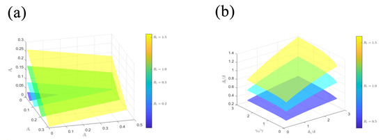
Figure 7. Three-dimensional curved surface of $R_t$. (a)The distribution of $R_t$ vary with ${\beta }_a$, ${\beta }_e$ and ${\beta }_i$. (b) The distribution of $R_t$ vary with $\beta$, $\delta$ and $\gamma$. $\beta$ represents the combined effect of ${\beta }_a$, ${\beta }_e$ and ${\beta }_i$. The stricter control policy corresponds to a smaller $\beta$.

8. Conclusions

To better simulate the dynamics of COVID-19 transmission, we developed a SEIAQR model incorporating the infections by asymptomatic patients as well as the population during the incubation period. The stability of the six-dimensional system was investigated by the Lyapunov method. As illustrated in the numerical simulation, different control strategies in Japan should lead to different final outcomes in view of the convergence points. Further, the sensitivity analysis was performed to analyze the impact of various transmission approaches on the disease spreading in the model. The parameters associated with the asymptomatic transmission could greatly affect the change of the effective reproduction number. Therefore, imposing effective containment policies to restrict asymptomatic infections should be of crucial significance as manifested by this work. The analysis using the system of ODEs offer general guidance on the containment of COVID-19 at a macro level, which lesser emphasizes the influence of spatial distribution. The dynamics of systems based on space-time PDEs will be explored in our future work to consider regional-related effects.

References

- Bernal, J.L.; Andrews, N.; Gower, C.; Gallagher, E.; Simmons, R.; Thelwall, S.; Stowe, J.; Tessier, E.; Groves, N.; Dabrera, G.; et al. Effectiveness of COVID-19 Vaccines against the B.1.617.2 (Delta) Variant. N. Engl. J. Med. 2021, 385, 585–594. [Google Scholar] [CrossRef]
- Korber, B.; Fischer, W.M.; Gnanakaran, S.; Yoon, H.; Theiler, J.; Abfalterer, W.; Hengartner, N.; Giorgi, E.E.; Bhattacharya, T.; Foley, B.; et al. Tracking Changes in SARS-CoV-2 Spike: Evidence that D614G Increases Infectivity of the COVID-19 Virus. Cell 2020, 182, 812–827.e19. [Google Scholar] [CrossRef] [PubMed]
- Tillett, R.L.; Sevinsky, J.R.; Hartley, P.D.; Kerwin, H.; Crawford, N.; Gorzalski, A.; Laverdure, C.; Verma, S.C.; Rossetto, C.C.; Jackson, D.; et al. Genomic evidence for reinfection with SARS-CoV-2: A case study. Lancet Infect. Dis. 2021, 21, 52–58. [Google Scholar] [CrossRef]
- Weisblum, Y.; Schmidt, F.; Zhang, F.W.; DaSilva, J.; Poston, D.; Lorenzi, J.C.C.; Muecksch, F.; Rutkowska, M.; Hoffmann, H.H.; Michailidis, E.; et al. Escape from neutralizing antibodies by SARS-CoV-2 spike protein variants. eLife 2020, 9, 31. [Google Scholar] [CrossRef]
- Bollyky, T.J.; Hull, E.N.; Barber, R.M.; Collins, J.K.; Kiernan, S.; Moses, M.; Pigott, D.M.; Reiner, R.C., Jr.; Sorensen, R.J.; Abbafati, C.; et al. Pandemic preparedness and COVID-19: An exploratory analysis of infection and fatality rates, and contextual factors associated with preparedness in 177 countries, from Jan 1, 2020, to Sept 30, 2021. Lancet, 2022; in press. Available online: https://www.sciencedirect.com/science/article/pii/S0140673622001726(accessed on 1 February 2022).
- Haug, N.; Geyrhofer, L.; Londei, A.; Dervic, E.; Desvars-Larrive, A.; Loreto, V.; Pinior, B.; Thurner, S.; Klimek, P. Ranking the effectiveness of worldwide COVID-19 government interventions. Nat. Hum. Behav. 2020, 4, 1303–1312. [Google Scholar] [CrossRef] [PubMed]
- Cohn, B.A.; Cirillo, P.M.; Murphy, C.C.; Krigbaum, N.Y.; Wallace, A.W. SARS-CoV-2 vaccine protection and deaths among US veterans during 2021. Science 2021, 375, 331–336. [Google Scholar] [CrossRef] [PubMed]
- Cao, Y.; Wang, J.; Jian, F.; Xiao, T.; Song, W.; Yisimayi, A.; Huang, W.; Li, Q.; Wang, P.; An, R. Omicron escapes the majority of existing SARS-CoV-2 neutralizing antibodies. Nature 2021, 602, 657–663. [Google Scholar] [CrossRef] [PubMed]
- Australia Moves to Lift COVID-19 Restrictions Amid Surge in Omicron Infections. Available online: https://www.cnn.com/2021/12/14/australia/australia-omicron-covid-outbreak-restrictions-intl-hnk/index.html (accessed on 15 December 2021).
- Slowing the Spread of the Omicron Variant: Lockdown in The Netherlands. Available online: https://www.government.nl/latest/news/2021/12/18/slowing-the-spread-of-the-omicron-variant-lockdown-in-the-netherlands (accessed on 18 December 2021).
- Chowell, G.; Hengartner, N.W.; Castillo-Chavez, C.; Fenimore, P.W.; Hyman, J.M. The basic reproductive number of Ebola and the effects of public health measures: The cases of Congo and Uganda. J. Theor. Biol. 2004, 229, 119–126. [Google Scholar] [CrossRef] [Green Version]
- Ciofi degli Atti, M.L.; Merler, S.; Rizzo, C.; Ajelli, M.; Massari, M.; Manfredi, P.; Furlanello, C.; Scalia Tomba, G.; Iannelli, M. Mitigation measures for pandemic influenza in Italy: An individual based model considering different scenarios. PLoS ONE 2008, 3, e1790. [Google Scholar] [CrossRef] [Green Version]
- Medley, G.; Lindop, N.; Edmunds, J.; Nokes, J. Hepatitis-B virus endemicity: Heterogeneity, catastrophic dynamics and control. Nat. Med. 2001, 7, 619–624. [Google Scholar] [CrossRef] [PubMed]
- Mills, C.; Robins, J.; Lipsitch, M. Transmissibility of 1918 pandemic influenza. Nature 2004, 432, 904–906. [Google Scholar] [CrossRef] [PubMed]
- Grassly, N.C.; Pons-Salort, M.; Parker, E.P.K.; White, P.J.; Ferguson, N.M.; Imperial Coll, C. Comparison of molecular testing strategies for COVID-19 control: A mathematical modelling study. Lancet Infect. Dis. 2020, 20, 1381–1389. [Google Scholar] [CrossRef]
- He, Z.; Ren, L.; Yang, J.; Guo, L.; Feng, L.; Ma, C.; Wang, X.; Leng, Z.; Tong, X.; Zhou, W.; et al. Seroprevalence and humoral immune durability of anti-SARS-CoV-2 antibodies in Wuhan, China: A longitudinal, population-level, cross-sectional study. Lancet 2021, 397, 1075–1084. [Google Scholar] [CrossRef]
- Lin, Q.Y.; Zhao, S.; Gao, D.Z.; Lou, Y.J.; Yang, S.; Musa, S.S.; Wang, M.G.H.; Cai, Y.L.; Wang, W.M.; Yang, L.; et al. A conceptual model for the coronavirus disease 2019 (COVID-19) outbreak in Wuhan, China with individual reaction and governmental action. Int. J. Infect. Dis. 2020, 93, 211–216. [Google Scholar] [CrossRef] [PubMed]
- Ndairoua, F.; Area, I.; Nieto, J.J.; Torres, D.F.M. Mathematical modeling of COVID-19 transmission dynamics with a case study of Wuhan. Chaos Solitons Fractals 2020, 135, 109846. [Google Scholar] [CrossRef] [PubMed]
- Wu, J.T.; Leung, K.; Leung, G.M. Nowcasting and forecasting the potential domestic and international spread of the 2019-nCoV outbreak originating in Wuhan, China: A modelling study. Lancet 2020, 395, 689–697. [Google Scholar] [CrossRef] [Green Version]
- Yi, N.; Zhang, Q.; Mao, K.; Yang, D.; Li, Q. Analysis and control of an SEIR epidemic system with nonlinear transmission rate. Math. Comput. Model. 2009, 50, 1498–1513. [Google Scholar] [CrossRef]
- Péni, T.; Szederkényi, G. Convex output feedback model predictive control for mitigation of COVID-19 pandemic. Annu. Rev. Control 2021, 52, 543–553. [Google Scholar] [CrossRef] [PubMed]
- Bhattacharjee, S.; Liao, S.; Paul, D.; Chaudhuri, S. Inference on the dynamics of COVID-19 in the United States. Sci. Rep. 2022, 12, 2253. [Google Scholar] [CrossRef]
- Wang, M.; Yi, J.; Jiang, W. Study on the virulence evolution of SARS-CoV-2 and the trend of the epidemics of COVID-19. Math. Methods Appl. Sci. 2022, 1–20. [Google Scholar] [CrossRef]
- Leontitsis, A.; Senok, A.; Alsheikh-Ali, A.; Al Nasser, Y.; Loney, T.; Alshamsi, A. Seahir: A specialized compartmental model for covid-19. Int. J. Environ. Res. Public Health 2021, 18, 2667. [Google Scholar] [CrossRef] [PubMed]
- Ukaj, N.; Scheiner, S.; Hellmich, C. Toward “hereditary epidemiology”: A temporal Boltzmann approach to COVID-19 fatality trends. Appl. Phys. Rev. 2021, 8, 041417. [Google Scholar] [CrossRef]
- Grave, M.; Viguerie, A.; Barros, G.F.; Reali, A.; Coutinho, A.L. Assessing the spatio-temporal spread of COVID-19 via compartmental models with diffusion in Italy, USA, and Brazil. Arch. Comput. Methods Eng. 2021, 28, 4205–4223. [Google Scholar] [CrossRef] [PubMed]
- Majid, F.; Deshpande, A.M.; Ramakrishnan, S.; Ehrlich, S.; Kumar, M. Analysis of epidemic spread dynamics using a PDE model and COVID-19 data from Hamilton County OH USA. IFAC-PapersOnLine 2021, 54, 322–327. [Google Scholar] [CrossRef]
- El Koufi, A.; El Koufi, N. Stochastic differential equation model of Covid-19: Case study of Pakistan. Results Phys. 2022, 34, 105218. [Google Scholar] [CrossRef] [PubMed]
- Niu, R.; Chan, Y.C.; Wong, E.W.; van Wyk, M.A.; Chen, G. A stochastic SEIHR model for COVID-19 data fluctuations. Nonlinear Dyn. 2021, 106, 1311–1323. [Google Scholar] [CrossRef]
- Angeli, M.; Neofotistos, G.; Mattheakis, M.; Kaxiras, E. Modeling the effect of the vaccination campaign on the COVID-19 pandemic. Chaos Solitons Fractals 2022, 154, 111621. [Google Scholar] [CrossRef] [PubMed]
- Gallo, L.; Frasca, M.; Latora, V.; Russo, G. Lack of practical identifiability may hamper reliable predictions in COVID-19 epidemic models. Sci. Adv. 2012, 8, eabg5234. [Google Scholar] [CrossRef] [PubMed]
- Meyerowitz, E.A.; Richterman, A.; Bogoch, I.; Low, N.; Cevik, M. Towards an accurate and systematic characterisation of persistently asymptomatic infection with SARS-CoV-2. Lancet Infect. Dis. 2021, 21, e163–e169. [Google Scholar] [CrossRef]
- Li, M.Y.; Muldowney, J.S. Global stability for the SEIR model in epidemiology. Math. Biosci. 1995, 125, 155–164. [Google Scholar] [CrossRef]
- Wangari, I.M. Condition for Global Stability for a SEIR Model Incorporating Exogenous Reinfection and Primary Infection Mechanisms. Comput. Math. Methods Med. 2020, 2020, 9435819. [Google Scholar] [CrossRef]
- Korobeinikov, A. Lyapunov functions and global stability for SIR and SIRS epidemiological models with non-linear transmission. Bull. Math. Biol. 2006, 68, 615–626. [Google Scholar] [CrossRef] [PubMed] [Green Version]
- Korobeinikov, A. Global properties of infectious disease models with nonlinear incidence. Bull. Math. Biol. 2007, 69, 1871–1886. [Google Scholar] [CrossRef] [PubMed]
- McCluskey, C.C. Lyapunov functions for tuberculosis models with fast and slow progression. Math. Biosci. Eng. 2006, 3, 603–614. [Google Scholar] [CrossRef] [PubMed]
- Melnik, A.V.; Korobeinikov, A. Lyapunov functions and global stability for SIR and SEIR models with age-dependent susceptibility. Math. Biosci. Eng. 2013, 10, 369–378. [Google Scholar] [CrossRef] [PubMed]
- Ahmed, I.; Modu, G.U.; Yusuf, A.; Kumam, P.; Yusuf, I. A mathematical model of Coronavirus Disease (COVID-19) containing asymptomatic and symptomatic classes. Results Phys. 2021, 21, 103776. [Google Scholar] [CrossRef] [PubMed]
- Annas, S.; Isbar Pratama, M.; Rifandi, M.; Sanusi, W.; Side, S. Stability analysis and numerical simulation of SEIR model for pandemic COVID-19 spread in Indonesia. Chaos Solitons Fractals 2020, 139, 110072. [Google Scholar] [CrossRef] [PubMed]
- Ansumali, S.; Kaushal, S.; Kumar, A.; Prakash, M.K.; Vidyasagar, M. Modelling a pandemic with asymptomatic patients, impact of lockdown and herd immunity, with applications to SARS-CoV-2. Annu. Rev. Control 2020, 50, 432–447. [Google Scholar] [CrossRef] [PubMed]
- Batabyal, S. COVID-19: Perturbation dynamics resulting chaos to stable with seasonality transmission. Chaos Solitons Fractals 2021, 145, 110772. [Google Scholar] [CrossRef] [PubMed]
- Jiao, J.; Liu, Z.; Cai, S. Dynamics of an SEIR model with infectivity in incubation period and homestead-isolation on the susceptible. Appl. Math. Lett. 2020, 107, 106442. [Google Scholar] [CrossRef] [PubMed]
- Youssef, H.M.; Alghamdi, N.A.; Ezzat, M.A.; El-Bary, A.A.; Shawky, A.M. A new dynamical modeling SEIR with global analysis applied to the real data of spreading COVID-19 in Saudi Arabia. Math. Biosci. Eng. 2020, 17, 7018–7044. [Google Scholar] [CrossRef] [PubMed]
- Khajji, B.; Kouidere, A.; Elhia, M.; Balatif, O.; Rachik, M. Fractional optimal control problem for an age-structured model of COVID-19 transmission. Chaos Solitons Fractals 2021, 143, 110625. [Google Scholar] [CrossRef]
- Zarin, R.; Khan, A.; Yusuf, A.; Abdel-Khalek, S.; Inc, M. Analysis of fractional COVID-19 epidemic model under Caputo operator. Math. Methods Appl. Sci. 2021, 2021, mma.7294. [Google Scholar] [CrossRef]
- Biala, T.A.; Khaliq, A.Q.M. A fractional-order compartmental model for the spread of the COVID-19 pandemic. Commun. Nonlinear Sci. Numer. Simul. 2021, 98, 105764. [Google Scholar] [CrossRef] [PubMed]
- Avila-Ponce de León, U.; Pérez Á, G.C.; Avila-Vales, E. An SEIARD epidemic model for COVID-19 in Mexico: Mathematical analysis and state-level forecast. Chaos Solitons Fractals 2020, 140, 110165. [Google Scholar] [CrossRef] [PubMed]
- Musa, S.S.; Baba, I.A.; Yusuf, A.; Sulaiman, T.A.; Aliyu, A.I.; Zhao, S.; He, D.H. Transmission dynamics of SARS-CoV-2: A modeling analysis with high-and-moderate risk populations. Results Phys. 2021, 26, 104290. [Google Scholar] [CrossRef]
- Samui, P.; Mondal, J.; Khajanchi, S. A mathematical model for COVID-19 transmission dynamics with a case study of India. Chaos Solitons Fractals 2020, 140, 110173. [Google Scholar] [CrossRef] [PubMed]
- Zamir, M.; Shah, K.; Nadeem, F.; Bajuri, M.Y.; Ahmadian, A.; Salahshour, S.; Ferrara, M. Threshold conditions for global stability of disease free state of COVID-19. Results Phys. 2021, 21, 103784. [Google Scholar] [CrossRef]
- Samsuzzoha, M.; Singh, M.; Lucy, D. Uncertainty and sensitivity analysis of the basic reproduction number of a vaccinated epidemic model of influenza. Appl. Math. Model. 2013, 37, 903–915. [Google Scholar] [CrossRef]
- Asamoah, J.K.K.; Jin, Z.; Sun, G.Q.; Seidu, B.; Yankson, E.; Abidemi, A.; Oduro, F.T.; Moore, S.E.; Okyere, E. Sensitivity assessment and optimal economic evaluation of a new COVID-19 compartmental epidemic model with control interventions. Chaos Solitons Fractals 2021, 146, 110885. [Google Scholar] [CrossRef] [PubMed]
- Hussain, T.; Ozair, M.; Ali, F.; Rehman, S.U.; Assiri, T.A.; Mahmoud, E.E. Sensitivity analysis and optimal control of COVID-19 dynamics based on SEIQR model. Results Phys. 2021, 22, 103956. [Google Scholar] [CrossRef]
- Islam, N.; Shkolnikov, V.M.; Acosta, R.J.; Klimkin, I.; Kawachi, I.; Irizarry, R.A.; Alicandro, G.; Khunti, K.; Yates, T.; Jdanov, D.A.; et al. Excess deaths associated with covid-19 pandemic in 2020: Age and sex disaggregated time series analysis in 29 high income countries. BMJ 2021, 373, n1137. [Google Scholar] [CrossRef] [PubMed]
- De León, C.V. Constructions of Lyapunov Functions for Classics SIS, SIR and SIRS Epidemic model with Variable Population Size. Foro-Red Rev. Electrónica Conten. Matemático 2009, 26, 1–12. [Google Scholar]
- Hethcote, H.W. Epidemiology models with variable population size. Math. Underst. Infect. Dis. Dyn. 2008, 16, 63. [Google Scholar]
- Van den Driessche, P.; Watmough, J. Reproduction numbers and sub-threshold endemic equilibria for compartmental models of disease transmission. Math. Biosci. 2002, 180, 29–48. [Google Scholar] [CrossRef]
- Zhou, K.; Doyle, J.C. Essentials of Robust Control; Prentice Hall: Upper Saddle River, NJ, USA, 1998; Volume 38. [Google Scholar]
- Butler, G.; Freedman, H.I.; Waltman, P. Uniformly persistent systems. Proc. Am. Math. Soc. 1986, 96, 425–430. [Google Scholar] [CrossRef]
- Zhao, X.Q. Dynamical Systems in Population Biology; Springer: Berlin/Heidelberg, Germany, 2003. [Google Scholar]
- Xu, D.G.; Xu, X.Y.; Yang, C.H.; Gui, W.H. Global Stability of a Variation Epidemic Spreading Model on Complex Networks. Math. Probl. Eng. 2015, 2015, 365049. [Google Scholar] [CrossRef] [Green Version]
- Hethcote, H.W.; Thieme, H.R. Stability of the endemic equilibrium in epidemic models with subpopulations. Math. Biosci. 1985, 75, 205–227. [Google Scholar] [CrossRef]
- Esteva, L.; Vargas, C. Influence of vertical and mechanical transmission on the dynamics of dengue disease. Math. Biosci. 2000, 167, 51–64. [Google Scholar] [CrossRef]
- Brodsky, A.R.; Krasnoselskii, M.A.; Flaherty, R.E.; Boron, L.F. Positive Solutions of Operator Equations. Am. Math. Mon. 1967, 74, 343. [Google Scholar] [CrossRef]
- Martcheva, M. An Introduction to Mathematical Epidemiology; Springer: Berlin/Heidelberg, Germany, 2015; Volume 61. [Google Scholar]
- Japan Population 1950–2022. Available online: https://www.macrotrends.net/countries/JPN/japan/population (accessed on 1 February 2022).
- Lauer, S.A.; Grantz, K.H.; Bi, Q.; Jones, F.K.; Zheng, Q.; Meredith, H.R.; Azman, A.S.; Reich, N.G.; Lessler, J. The Incubation Period of Coronavirus Disease 2019 (COVID-19) From Publicly Reported Confirmed Cases: Estimation and Application. Ann. Intern. Med. 2020, 172, 577–582. [Google Scholar] [CrossRef] [PubMed] [Green Version]
- Zheng, X. Asymptomatic patients and asymptomatic phases of Coronavirus Disease 2019 (COVID-19): A population-based surveillance study. Natl. Sci. Rev. 2020, 7, 1527–1539. [Google Scholar] [CrossRef] [PubMed]
- Japan Coronavirus Data List. Available online: https://www3.nhk.or.jp/news/special/coronavirus/data-widget/ (accessed on 30 December 2021).
- Vidyullatha, P.; Rao, D.R. Machine learning techniques on multidimensional curve fitting data based on R-square and chi-square methods. Int. J. Electr. Comput. Eng. 2016, 6, 974. [Google Scholar]
- Capaldi, A.; Behrend, S.; Berman, B.; Smith, J.; Wright, J.; Lloyd, A.L. Parameter estimation and uncertainty quantification for an epidemic model. Math. Biosci. Eng. 2012, 9, 553–576. [Google Scholar] [PubMed]
Publisher’s Note: MDPI stays neutral with regard to jurisdictional claims in published maps and institutional affiliations. |
© 2022 by the authors. Licensee MDPI, Basel, Switzerland. This article is an open access article distributed under the terms and conditions of the Creative Commons Attribution (CC BY) license (https://creativecommons.org/licenses/by/4.0/).