Stability Analysis and Computational Interpretation of an Effective Semi Analytical Scheme for Fractional Order Non-Linear Partial Differential Equations

Abstract

In this study we will check the stability of the semi analytical technique, the Laplace variational iteration (LVI) scheme, which is the combination of a variational iteration technique and the Laplace transform method. Then, we will apply it to solve some non-linear fractional order partial differential equations. Since the Laplace transform cannot be applied to non-linear problems, the combination of the variational iteration technique with it will give a better and rapidly convergent sequence. Exact solutions may also exist, but we will show that the coupled technique is much better to approximate the exact solutions. The Caputo–Fabrizio fractional derivative will be used throughout the study. In addition, some possible implications of the results given here are connected with fixed point theory.

1. Introduction and Preliminaries

It is being observed that some non-linear differential equations are used in the modelling of some well-known physical phenomena in science and engineering, and we refer to the Korteweg–de Vries (KdV) equation [1,2], Schrödinger equation [3,4,5], nonlinear advection–diffusion–reaction problems [6,7], nonlinear Burger’s equation [8], nonlinear Riccati systems [9] and Sobolev type Volterra–Fredholm integro-differential system [10] etc.

The previously mentioned differential equations/systems and others are solved by using more than one analytical, semi-analytical and numerical method such as Hirota’s bilinear method [11,12], the Laplace transform method (LTM) [13,14], variational iteration method (VIM) [15,16], Adomian decomposition method (ADM) [17], Newton–Raphson formula (NRF) [18] and the spectral collocation technique (SCT) [19,20,21,22].

Recently, fractional calculus is being used instead of ordinary calculus in order to understand real world phenomena more precisely. It has gained a special place in the modelling of physical, economical and biological phenomena due to its memory effects. The recent trend in the study of natural phenomena is to use the Laplace transform to solve the ODEs with constant and variable coefficients and, at the same time, to solve PDEs. Likewise, in the last decades, the method variational iteration technique, given by the Chinese mathematician J. He-Huan [16], proved to be a very useful tool for solving PDEs. We must mention that the original method of J. He-Huan was drafted for searching solutions of integral and integro-differential equations. The limitations of the variational iteration method appears in the calculation of the Lagrange multiplier.

At present, to get better results quickly, a combination of more than one technique is being used to solve a model, especially non-linear models (see [23,24]).

In the present study, we use two techniques: the variational iteration technique and the Laplace transform. Then the combined technique, the Laplace variational iteration (LVI), is used to deal with non-linear fractional order partial differential equations (FOPDEs). The big advantage of this method is the faster convergence compared with the existing one, to solve FOPDEs. The utilization of it introduces a new significant innovation in the study of FOPDEs. In this direction, J. Iqbal et al. introduced in [25] the combined technique variational iteration transform method (VITM) in order to solve non-linear fractional order partial differential equations such as Burger’s equation [26], the Korteweg–de Vries equation [27] and the Schrödinger equation [28].

The Caputo–Fabrizio fractional derivative operator is one of the most used fractional derivatives in the study of initial value problems. In our further study of the fractional differential equations, the Caputo–Fabrizio fractional derivative [29] will be considered.

Then, let us give some crucial definitions from fractional calculus field.

Definition 1.

The Riemann–Liouville fractional derivative of a function $f\left(\overline{t}\right)$ is defined to be,

$$D^{\alpha }f\left(\overline{t}\right)={\left(\frac{d}{d\overline{t}}\right)}^{\overline{\epsilon }+1}{\int }_a^{\overline{t}}{(\overline{t}-\tau )}^{\overline{\epsilon }-\alpha }f\left(\tau \right)d\tau ,$$

(1)

where $\overline{\epsilon }\le \alpha <\overline{\epsilon }+1$

• or

$$D^{\alpha }f\left(\overline{t}\right)=\frac{1}{\Gamma (\kappa -\alpha )}\frac{d^{\kappa }}{d{\overline{t}}^{\kappa }}{\int }_a^{\overline{t}}{(\overline{t}-\tau )}^{\kappa -\alpha -1}f\left(\tau \right)d\tau ,$$

(2)

where $\kappa -1\le \alpha <\kappa$. Both κ and $\overline{\epsilon }$ are integers.

Definition 2.

The Caputo’s fractional derivative of $f\left(\overline{t}\right)$ is given by:

$$D_a^{\alpha }f\left(\overline{t}\right)=\frac{1}{\Gamma (1-\alpha )}{\int }_a^{\overline{t}}\frac{f^{\prime }(\overline{t}-\tau )}{{(\tau -a)}^{\alpha }}d\tau ,$$

(3)

such that $\alpha \in [0,1]$.

Note that under natural conditions on $f\left(\overline{t}\right)$ and $\alpha \to n$, the Caputo fractional derivative becomes the ordinary n-th order derivative.

We recall the fractional derivative Caputo–Fabrizio derivative, as follows.

Definition 3.

Let $\mathcal{F}\left(\overline{t}\right)\in H^1(a,b),b>a$; then the Caputo–Fabrizio time fractional derivative of $\mathcal{F}\left(\overline{t}\right)$ is defined as:

$${}_0^{CF}{D}_t^{\alpha }\mathcal{F}\left(\overline{t}\right)=\frac{\mathcal{M}\left(a\right)}{(1-\alpha )}{\int }_a^{\overline{t}}{\mathcal{F}}^{\prime }\left(\overline{t}\right)\exp [-\frac{\alpha (\overline{t}-\tau )}{1-\alpha }]d\tau ,$$

(4)

where $\alpha \in [0,1]$ and $\mathcal{M}\left(a\right)$ is a normalization function that is $\mathcal{M}\left(0\right)=\mathcal{M}\left(1\right)=1$.

Definition 4.

Let $f\left(\overline{t}\right)$ be a function, then its Laplace transform is defined as:

$$\mathcal{L}\left\{f\left(\overline{t}\right)\right\}=\mathcal{F}\left(\overline{s}\right)={\int }_0^{\infty }{e}^{-\overline{s}\overline{t}}f\left(\overline{t}\right)d\overline{t},$$

(5)

and the Laplace transform of $f\left(\overline{t}\right)$ in the Caputo–Fabrizio sense is given by [30]:

$$\mathcal{L}\left\{D_{\overline{t}}^{(\alpha +n)}f\left(\overline{t}\right)\right\}=\frac{{\overline{s}}^{(n+1)}\mathcal{L}\left[f\left(\overline{t}\right)\right]-{\overline{s}}^{n}f\left(0\right)-{\overline{s}}^{n-1}{f}^{\prime }\left(0\right)-\dots -f^{\left(n\right)}\left(0\right)}{\overline{s}+\alpha (1-\overline{s})}.$$

(6)

For $n=0$, we have:

$$\mathcal{L}\left\{D_{\overline{t}}^{\left(\alpha \right)}f\left(\overline{t}\right)\right\}=\frac{\overline{s}\mathcal{L}\left[f\left(\overline{t}\right)\right]-f\left(0\right)}{\overline{s}+\alpha (1-\overline{s})}.$$

(7)

In this paper we introduce a new semi analytical technique Laplace variational iteration (LVI) scheme, which is the combination of a variational iteration technique and the Laplace transform method. Then, we will check the stability of the new proposed scheme, creating in this way a close connection with the field of fixed point theory. We will give some examples to put in evidence the advantages of our proposed scheme with respect to existing ones from related literature. The accuracy and the yield of the LVI scheme are evidenced by some 3D-graphical display, with the help of the software $Mathematic{a}^{TM}$-version 11.1.

Moreover, we will highlight the usefulness of the semi analytical method, which gives the best approximations of the exact solution of partial differential equations, especially of fractional order nonlinear partial differential equations, which are difficult to solve.

2. Basis of the Laplace Variational Iteration Method

This section is focused on presenting the basis of the Laplace variational iteration method. For this, recall the general time fractional partial differential equation.

$$\begin{array}{cc}\hfill & D_{\overline{t}}^{\alpha }\mathcal{X}(\overline{\phi },\overline{t})+L\left(\mathcal{X}(\overline{\phi },\overline{t})\right)+N\left(\mathcal{X}(\overline{\phi },\overline{t}),\mathcal{Y}(\overline{\phi },\overline{t}),\mathcal{Z}(\overline{\phi },\overline{t})\right)=\mathcal{F}(\overline{\phi },\overline{t});\hfill \end{array}$$

(8)

subject to

$$\mathcal{X}(\overline{\phi },0)={\mathcal{X}}_0,$$

where $L\left(\mathcal{X}(\overline{\phi },\overline{t})\right)$, $N\left(\mathcal{X}(\overline{\phi },\overline{t}),\mathcal{Y}(\overline{\phi },\overline{t}),\mathcal{Z}(\overline{\phi },\overline{t})\right)$ and $\mathcal{F}(\overline{\phi },\overline{t})$ are linear, nonlinear and known functions, respectively. Additionally, we consider $D_{\overline{t}}^{\alpha }$ in the Caputo–Fabrizio sense.

Applying the variational iteration method in Equation (8) we get:

$$\begin{array}{cc}\hfill {\mathcal{X}}_{n+1}(\overline{\phi },\overline{t})=& {\mathcal{X}}_n(\overline{\phi },\overline{t})+\lambda \{D_{\overline{t}}^{\alpha }\mathcal{X}(\overline{\phi },\overline{t})+L\left(\mathcal{X}(\overline{\phi },\overline{t})\right)\hfill \\ \hfill & +N\left(\mathcal{X}(\overline{\phi },\overline{t}),\mathcal{Y}(\overline{\phi },\overline{t}),\mathcal{Z}(\overline{\phi },\overline{t})\right)-\mathcal{F}(\overline{\phi },\overline{t})\}.\hfill \end{array}$$

Additionally, applying the Laplace transform, the variable t becomes a new ones, such that:

$$\begin{array}{cc}\hfill {\mathcal{X}}_{n+1}(\overline{\phi },\overline{s})=& {\mathcal{X}}_n(\overline{\phi },\overline{s})+\lambda \mathcal{L}\{D_{\overline{t}}^{\alpha }{\mathcal{X}}_n(\overline{\phi },\overline{t})+L{\tilde{\mathcal{X}}}_n(\overline{\phi },\overline{t})\hfill \\ \hfill & +N({\tilde{\mathcal{X}}}_n(\overline{\phi },\overline{t}),{\tilde{\mathcal{Y}}}_n(\overline{\phi },\overline{t}),{\tilde{\mathcal{Z}}}_n(\overline{\phi },\overline{t}))-\mathcal{F}(\overline{\phi },\overline{t})\},\hfill \end{array}$$

(9)

where ${\tilde{\mathcal{X}}}_n(\overline{\phi },\overline{t})$ etc. are restricted values, which means

$$\delta {\tilde{\mathcal{X}}}_n(\overline{\phi },\overline{t})=0.$$

Using relation Equation (7) we get:

$$\mathcal{L}\left\{D^{\alpha }{\mathcal{X}}_n(\overline{\phi },\overline{t})\right\}=\frac{\overline{s}{\mathcal{X}}_n(\overline{\phi },\overline{s})-{\mathcal{X}}_n(\overline{\phi },0)}{\overline{s}+\alpha (1-\overline{s})}$$

and

$$\mathcal{L}\left\{\delta D^{\alpha }{\mathcal{X}}_n(\overline{\phi },\overline{t})\right\}=\frac{s\delta {\mathcal{X}}_n(\overline{\phi },\overline{s})-\delta {\mathcal{X}}_n(\overline{\phi },0)}{\overline{s}+\alpha (1-\overline{s})},$$

where

$$\delta {\mathcal{X}}_n(\overline{\phi },0)=0.$$

Then, we obtain:

$$\mathcal{L}\left\{\delta D^{\alpha }{\mathcal{X}}_n(\overline{\phi },\overline{t})\right\}=\frac{s\delta {\mathcal{X}}_n(\overline{\phi },\overline{s})}{\overline{s}+\alpha (1-\overline{s})}.$$

From the optimization conditions,

$$\frac{\delta {\tilde{\mathcal{X}}}_{n+1}(\overline{\phi },\overline{s})}{\delta {\tilde{\mathcal{X}}}_n(\overline{\phi },\overline{s})}=0$$

and

$$\delta \widetilde{{\mathcal{X}}_n}=0,\delta \widetilde{{\mathcal{Y}}_n}=0,\delta \widetilde{{\mathcal{Z}}_n}=0,$$

we get

$$0=1+\lambda \left\{\frac{\overline{s}\delta {\tilde{\mathcal{X}}}_n(\overline{\phi },\overline{s})}{(\overline{s}+\alpha (1-\overline{s}))\delta {\tilde{\mathcal{X}}}_n(\overline{\phi },\overline{s})}\right\}.$$

The above equation gives $\lambda =-\frac{\overline{s}+\alpha (1-\overline{s})}{\overline{s}}$.

Replacing Equation (9), we obtain:

$$\begin{array}{cc}\hfill {\mathcal{X}}_{n+1}(\overline{\phi },\overline{s})=& {\mathcal{X}}_n(\overline{\phi },\overline{s})-\left\{\frac{\overline{s}+\alpha (1-\overline{s})}{\overline{s}}\right\}\mathcal{L}\{D_{\overline{t}}^{\alpha }{\mathcal{X}}_n(\overline{\phi },\overline{t})+L{\tilde{\mathcal{X}}}_n(\overline{\phi },\overline{t})\hfill \\ \hfill & +N({\tilde{\mathcal{X}}}_n(\overline{\phi },\overline{t}),{\tilde{\mathcal{Y}}}_n(\overline{\phi },\overline{t}),{\tilde{\mathcal{Z}}}_n(\overline{\phi },\overline{t}))-\mathcal{F}(\overline{\phi },t)\}.\hfill \end{array}$$

Using the inverse Laplace transform we get:

$$\begin{array}{cc}\hfill {\mathcal{X}}_{n+1}(\overline{\phi },\overline{t})=& {\mathcal{X}}_n(\overline{\phi },\overline{t})-{\mathcal{L}}^{-1}\left\{\right\{\frac{\overline{s}+\alpha (1-\overline{s})}{\overline{s}}\left\}\mathcal{L}\right\{D_{\overline{t}}^{\alpha }{\mathcal{X}}_n(\overline{\phi },\overline{t})+L{\mathcal{X}}_n(\overline{\phi },\overline{t})\hfill \\ \hfill & +N({\mathcal{X}}_n(\overline{\phi },\overline{t}),{\mathcal{Y}}_n(\overline{\phi },\overline{t}),{\mathcal{Z}}_n(\overline{\phi },\overline{t}))-\mathcal{F}(\overline{\phi },\overline{t})\left\}\right\}.\hfill \end{array}$$

Replacing $n = 0, 1, 2, \dots$ we get the following successive approximations, ${\mathcal{X}}_1, {\mathcal{X}}_2, {\mathcal{X}}_3\dots ,$ which converge to exact solution, i.e., $\mathcal{X}=\underset{n\to \infty }{lim}{\mathcal{X}}_n.$

3. Stability Analysis of the Laplace Variational Iteration Scheme

Many stability notions have been developed in the last few decades, among which are Ulam–Hyers stability [31], Lyapunov stability [32], exponential stability [33], Mittag–Leffler stability [34] and so on. Then, we use the Banach contraction principle (see [35,36]) to check the stability of the proposed Laplace variational iteration (LVI). For this, let us recall some main definitions from fixed point theory.

Definition 5.

(Contraction mapping) Let $({\mathcal{P}}^{*},d)$ be a metric space. A mapping $\mathcal{S}:{\mathcal{P}}^{*}\to {\mathcal{P}}^{*}$ is said to be a contraction mapping, if for all $p_1^{*},p_2^{*}\in {\mathcal{P}}^{*}$ and a positive real constant $K<1$ we have:

$$d(\mathcal{S}{p}_1^{*},\mathcal{S}{p}_2^{*})\le Kd(p_1^{*},p_2^{*}).$$

(10)

This means that any pair of points $p_1^{*},p_2^{*}\in {\mathcal{P}}^{*}$ have images closer than the points $p_1^{*},p_2^{*}$ or, in other words, the ratio,

$$\frac{d(\mathcal{S}{p}_1^{*},\mathcal{S}{p}_2^{*})}{d(p_1^{*},p_2^{*})},$$

does not exceed a positive constant K, which is less than one (see [36]).

Further, let us recall the Picard’s existence and uniqueness theorem for differential equations. So we consider the following initial value problem:

$${\mathcal{X}}^{\prime }=\mathcal{S}(\overline{t},\mathcal{X}),withtheinitialcondition\mathcal{X}\left(\overline{t_0}\right)={\mathcal{X}}_0,$$

(11)

with $\overline{t_0}$ and ${\mathcal{X}}_0$ two given real numbers.

Let $\mathcal{S}$ be a continuous mapping on the rectangle,

$$R=\left\{(\overline{t},\mathcal{X})\right||\overline{t}-\overline{t_0}|\le a,|\mathcal{X}-{\mathcal{X}}_0|\le b\}.$$

Thus, $\mathcal{S}$ is bounded on R (see Figure 1). Then, for all $(\overline{t},\mathcal{X})\in R$, we can write:

$$\left|\mathcal{S}\right(\overline{t},\mathcal{X}\left)\right|\le c.$$

The behaviour of R with respect to the values of the parameters a, b and c can be seen in the Figure 2: (A)-for $a<\frac{b}{c}$, respectively (B)-for $a>\frac{b}{c}$.

Suppose that $\mathcal{S}$ satisfies the Lipschitz condition on R with respect to its second argument. Then, there exists a Lipschitz constant K such that, for all $(\overline{t},\mathcal{X}),(\overline{t},\mathcal{Y})\in R$,

$$|\mathcal{S}(\overline{t},\mathcal{X})-\mathcal{S}(\overline{t},\mathcal{Y})|\le K|\mathcal{X}-\mathcal{Y}|.$$

(12)

In these conditions, the above initial value problem Equation (11) has a unique solution in the interval $\{\overline{t_0}-\beta ,\overline{t_0}+\beta \}$, where $\beta <\{a,\frac{b}{c},\frac{1}{K}\}$ (see [36]).

Now, considering the above discussion we check the stability of LVI as follows:

$$\begin{array}{cc}\hfill {\mathcal{X}}_{n+1}=& \mathcal{S}\left({\mathcal{X}}_{n+1}\right)={\mathcal{X}}_n-{\mathcal{L}}^{-1}\left\{\right\{\frac{\overline{s}+\alpha (1-\overline{s})}{\overline{s}}\left\}\mathcal{L}\right\{D_{\overline{t}}^{\alpha }{\mathcal{X}}_n(\overline{\phi },\overline{t})+L{\mathcal{X}}_n(\overline{\phi },\overline{t})\hfill \\ \hfill & +N({\mathcal{X}}_n(\overline{\phi },\overline{t}),{\mathcal{Y}}_n(\overline{\phi },\overline{t}),{\mathcal{Z}}_n(\overline{\phi },\overline{t}))-\mathcal{F}(\overline{\phi },\overline{t})\left\}\right\}.\hfill \end{array}$$

Then we have:

$$\begin{array}{cc}\hfill |\mathcal{S}\left({\mathcal{X}}_{n+1}\right)-\mathcal{S}\left({\mathcal{X}}_{m+1}\right)|& \le |{\mathcal{X}}_n-{\mathcal{X}}_m|-{\mathcal{L}}^{-1}\left\{\right\{\frac{\overline{s}+\alpha (1-\overline{s})}{\overline{s}}\left\}\mathcal{L}\right\{D_{\overline{t}}^{\alpha }({\mathcal{X}}_n-{\mathcal{X}}_m)\hfill \\ \hfill & +L({\mathcal{X}}_n-{\mathcal{X}}_m)+N(({\mathcal{X}}_n-{\mathcal{X}}_m),({\mathcal{Y}}_n-{\mathcal{Y}}_m),({\mathcal{Z}}_n-{\mathcal{Z}}_m))\left\}\right\},\hfill \end{array}$$

which implies,

$$\begin{array}{cc}\hfill \frac{|\mathcal{S}\left({\mathcal{X}}_{n+1}\right)-\mathcal{S}\left({\mathcal{X}}_{m+1}\right)|}{|{\mathcal{X}}_n-{\mathcal{X}}_m|}& \le 1+{\mathcal{L}}^{-1}\left\{\right\{\frac{\overline{s}+\alpha (1-\overline{s})}{\overline{s}}\left\}\mathcal{L}\right\{D_{\overline{t}}^{\alpha }\left(\right|{\mathcal{X}}_n-{\mathcal{X}}_m\left|\right)\hfill \\ \hfill & +L\left(\right|{\mathcal{X}}_n-{\mathcal{X}}_m\left|\right)+N\left(\right|({\mathcal{X}}_n-{\mathcal{X}}_m),({\mathcal{Y}}_n-{\mathcal{Y}}_m),\left({\mathcal{Z}}_n\right)-{\mathcal{Z}}_m\left|\right)\left\}\right\}\hfill \\ \hfill & =K.\hfill \end{array}$$

Then, we obtain:

$$\frac{|\mathcal{S}\left({\mathcal{X}}_{n+1}\right)-\mathcal{S}\left({\mathcal{X}}_{m+1}\right)|}{|{\mathcal{X}}_n-{\mathcal{X}}_m|}\le K,$$

which means

$$|\mathcal{S}\left({\mathcal{X}}_{n+1}\right)-\mathcal{S}\left({\mathcal{X}}_{m+1}\right)|\le K\left(\right|{\mathcal{X}}_n-{\mathcal{X}}_m\left|\right).$$

Then, the proposed scheme is stable unconditionally by Equation (12).

4. Applications of Laplace Variational Iteration (LVI) Scheme on Various FODEs Types

In this section we apply the LVI scheme on some important FOPDEs from the related literature. Applying our stability scheme to some nonlinear fractional order models we prove how it approaches the exact solutions.

In this direction, our first application takes into consideration the most general time fractional form of the Korteweg–de Vries equation. It was first introduced by Boussinesq (1877) and also studied by Korteweg and de Vries (1895). The KdV equation is a mathematical model describing the behaviour of shallow water waves, especially long waves in the canals. The different forms of KdV equations have received the attention of researchers and a lot of numerical as well as analytical and semi analytical methods have been developed to deal with them (see [17,24]).

Now consider the general KdV equation in fractional form,

$$D_{\overline{t}}^{\alpha }\mathcal{X}+{\alpha }_1\mathcal{X}{\mathcal{X}}_{\overline{\phi }}+{\beta }_1{\mathcal{X}}_{\overline{\phi }\overline{\phi }\overline{\phi }}=0;0<\alpha \le 1,$$

(13)

subject to:

$$\mathcal{X}(\overline{\phi },0)={\mathcal{X}}_0=\frac{a}{{\cosh }^2{\beta }_1\overline{\phi }},$$

where

$${\alpha }_1=\frac{c_0}{2k^2}\left(ϵc{\lambda }_3\right)$$

is the nonlinear parameter and

$${\beta }_1=\frac{c_0{h}^2}{6}$$

is the dispersion parameter.

If we apply the proposed scheme on the above equation yields,

$$\begin{array}{cc}\hfill {\mathcal{X}}_{n+1}(\overline{\phi },\overline{t})& ={\mathcal{X}}_n(\overline{\phi },\overline{t})-{\mathcal{L}}^{-1}\left\{\frac{\overline{s}+\alpha (1-\overline{s})}{\overline{s}}\mathcal{L}\right\{D_{\overline{t}}^{\alpha }{\mathcal{X}}_n(\overline{\phi },\overline{t})\hfill \\ \hfill & +{\alpha }_1{\mathcal{X}}_n(\overline{\phi },\overline{t})\frac{\partial {\mathcal{X}}_n(\overline{\phi },\overline{t})}{\partial \overline{\phi }}+{\beta }_1\frac{{\partial }^3\mathcal{X}n(\overline{\phi },\overline{t})}{\partial {\overline{\phi }}^3}\left\}\right\}.\hfill \end{array}$$

If we take $n = 0, 1, 2, \dots$ we get the approximations ${\mathcal{X}}_1, {\mathcal{X}}_2, {\mathcal{X}}_3\dots$

The solution $\mathcal{X}(\overline{\phi },\overline{t})$ can be found as $\mathcal{X}(\overline{\phi },\overline{t})=\underset{i\to \infty }{lim}{\mathcal{X}}_i.$

As particular examples, let us consider further some versions of time fractional equations.

Example 1.

The first particular example is a simple time fractional Korteweg–de Vries equation (KdV equation). For more information about the different forms of KdV equations we refer to [17].

Consider,

$$D_{\overline{t}}^{\alpha }\mathcal{X}-6\mathcal{X}{\mathcal{X}}_{\overline{\phi }}+{\mathcal{X}}_{\overline{\phi }\overline{\phi }\overline{\phi }}=0;\mathcal{X}(\overline{\phi },0)=\frac{1}{6}(\overline{\phi }-1).$$

(14)

If we apply the proposed LVI scheme stepwise, we have:

$${\mathcal{X}}_{n+1}(\overline{\phi },\overline{s})={\mathcal{X}}_n(\overline{\phi },\overline{s})+\mathcal{L}\{\lambda \{D_{\overline{t}}^{\alpha }\widetilde{{\mathcal{X}}_n}(\overline{\phi },\overline{s})-6\widetilde{{\mathcal{X}}_n}(\overline{\phi },\overline{s})\frac{\partial \widetilde{{\mathcal{X}}_n}(\overline{\phi },\overline{s})}{\partial \overline{\phi }}+\frac{{\partial }^3\widetilde{{\mathcal{X}}_n}(\overline{\phi },\overline{s})}{\partial {\overline{\phi }}^3}\}\}.$$

The optimality conditions give the following results:

$$\frac{\delta {\tilde{\mathcal{X}}}_{n+1}(\overline{\phi },\overline{s})}{\delta {\tilde{\mathcal{X}}}_n(\overline{\phi },\overline{s})}=0,\delta \widetilde{{\mathcal{X}}_n}=0and\lambda =-\frac{\overline{s}+\alpha (1-\overline{s})}{\overline{s}}.$$

Replacing and using inverse Laplace transform we get:

$$\begin{array}{cc}\hfill {\mathcal{X}}_{n+1}(\overline{\phi },\overline{t})& ={\mathcal{X}}_n(\overline{\phi },\overline{t})-{\mathcal{L}}^{-1}\left\{\frac{\overline{s}+\alpha (1-\overline{s})}{\overline{s}}\mathcal{L}\right\{D_{\overline{t}}^{\alpha }{\mathcal{X}}_n(\overline{\phi },\overline{s})\hfill \\ & -6{\mathcal{X}}_n(\overline{\phi },\overline{s})\frac{\partial {\mathcal{X}}_n(\overline{\phi },\overline{s})}{\partial \overline{\phi }}+\frac{{\partial }^3\mathcal{X}n(\overline{\phi },\overline{s})}{\partial {\overline{\phi }}^3}\left\}\right\}.\hfill \end{array}$$

For $n = 0, 1, 2, \dots$ we get the approximations ${\mathcal{X}}_1, {\mathcal{X}}_2, {\mathcal{X}}_3\dots$ such as:

$${\mathcal{X}}_1(\overline{\phi },\overline{t})=\frac{1}{6}(\overline{\phi }-1)-\frac{1}{6}(1-\overline{\phi })(1-\alpha +\overline{t}\alpha )$$

and

$$\begin{array}{cc}\hfill {\mathcal{X}}_2(\overline{\phi },\overline{t})& =\frac{1}{6}(\overline{\phi }-1)-\frac{1}{6}(1-\overline{\phi })(1-\alpha +\overline{t}\alpha )\hfill \\ \hfill & -\frac{1}{6}\overline{t}(8\alpha -8\overline{\phi }\alpha -11{\alpha }^2+11\overline{\phi }{\alpha }^2+3{\alpha }^3-3\overline{\phi }{\alpha }^3)-\dots \hfill \end{array}$$

and so on.

The solution $\mathcal{X}(\overline{\phi },\overline{t})$ is obtained as $\mathcal{X}(\overline{\phi },\overline{t})=\underset{i\to \infty }{lim}{\mathcal{X}}_i$, i.e.,

$$\begin{array}{cc}\hfill \mathcal{X}(\overline{\phi },\overline{t})& =\frac{1}{6}(\overline{\phi }-1)-\frac{1}{6}(1-\overline{\phi })(1-\alpha +\overline{t}\alpha )\hfill \\ \hfill & -\frac{1}{6}\overline{t}(8\alpha -8\overline{\phi }\alpha -11{\alpha }^2-11\overline{\phi }{\alpha }^2+3{\alpha }^3-3\overline{\phi }{\alpha }^3)-\dots .\hfill \end{array}$$

For $\alpha =1$ we get $\mathcal{X}(\overline{\phi },\overline{t})=\frac{1}{6}(\overline{\phi }-1)-\frac{1}{6}\overline{t}(1-\overline{\phi })-\frac{1}{6}{\overline{t}}^2(1-\overline{\phi })-\frac{1}{18}{\overline{t}}^3(1-\overline{\phi }),$ which is the expansion of the exact solution $\mathcal{X}(\overline{\phi },\overline{t})=\frac{1}{6}\left(\frac{\overline{\phi }-1}{1-\overline{t}}\right)$ (see [17]), which confirms the validity of the proposed LVI scheme).

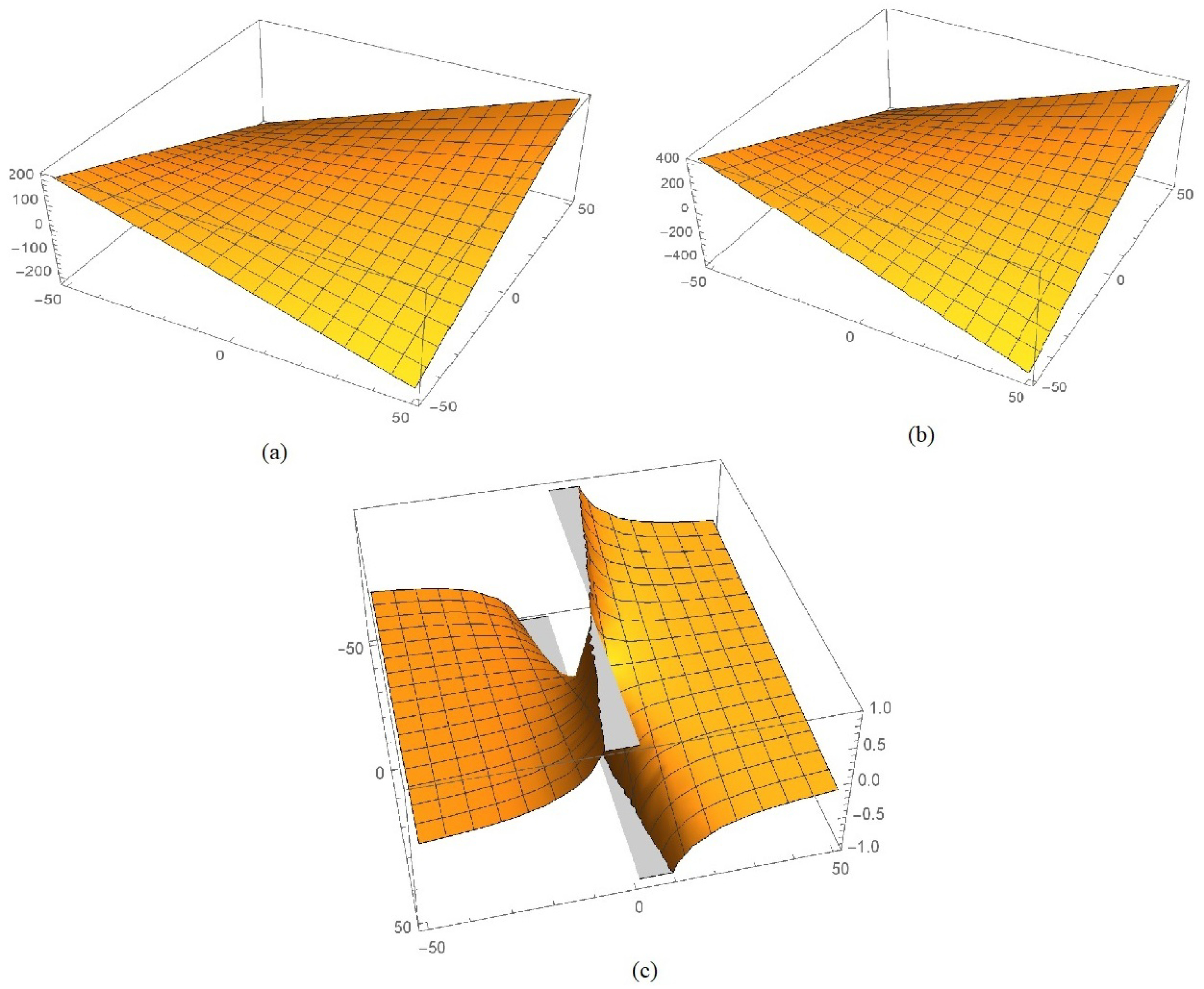
We next give a graphic 3D-display of the approximated solution, $\mathcal{X}(\overline{\phi },\overline{t})$, for various values of $\alpha$, using the computer software $Mathematic{a}^{TM}$-version 11.1. Then, we represent graphically a 3D-display of the exact solution $\mathcal{X}(\overline{\phi },\overline{t})=\frac{1}{6}\left(\frac{\overline{\phi }-1}{1-\overline{t}}\right)$, in Figure 3c, which demonstrates how the proposed scheme reaches the exact solution; see Figure 3a,b, which shows the approximations of Figure 3c.

As we know, the Korteweg–de Vries equation is the mathematical description of the shallow water waves, traveling in the canals or near the sea shores where water is not deep. The solution of Korteweg–de Vries equation describes the behavior of the shallow water waves, which helps us in designing the harbors and buildings and many other processes, near sea shores. Then, for such a solution we proposed the LVI scheme and we gave the previous 3D graphic.

As a second example, let us consider the simple time fractional Burger’s equation. It was introduced by Harry Bateman in 1915 and studied by J. M. Burger in 1948. It is considered one of the fundamental non-linear mathematical models in fluid dynamics that demonstrates the coupling between diffusion and convection.

The standard form of Burger’ s equation is as follows:

$$D_{\overline{t}}^{\alpha }\mathcal{X}+\mathcal{X}{\mathcal{X}}_{\overline{\phi }}+\nu {\mathcal{X}}_{\overline{\phi }\overline{\phi }}=0;\overline{t}>0,$$

(15)

where $\nu$ is a constant that defines the kinematic viscosity. Moreover if $\nu =0$, the equation is said to be inviscid that governs gas dynamics and traffic flow, discussed as a homogeneous advection problem, (see [17]).

Example 2.

Let us consider the Burger’s equation with $\nu =1$:

$$D_{\overline{t}}^{\alpha }\mathcal{X}+\mathcal{X}{\mathcal{X}}_{\overline{\phi }}+\mathcal{X}\overline{\phi }\overline{\phi }=0;\mathcal{X}(\overline{\phi },0)=1-\frac{2}{\overline{\phi }}.$$

(16)

Applying the proposed LVI scheme we have:

$${\mathcal{X}}_{n+1}(\overline{\phi },\overline{s})={\mathcal{X}}_n(\overline{\phi },\overline{s})+\mathcal{L}\{\lambda \{D_{\overline{t}}^{\alpha }\widetilde{{\mathcal{X}}_n}(\overline{\phi },\overline{s})+\widetilde{{\mathcal{X}}_n}(\overline{\phi },\overline{s})\frac{\partial \widetilde{{\mathcal{X}}_n}(\overline{\phi },\overline{s})}{\partial \overline{\phi }}+\frac{{\partial }^2\widetilde{{\mathcal{X}}_n}(\overline{\phi },\overline{s})}{\partial {\overline{\phi }}^2}\}\}.$$

The optimality conditions give the following results:

$$\frac{\delta {\tilde{\mathcal{X}}}_{n+1}(\overline{\phi },\overline{s})}{\delta \widetilde{{\mathcal{X}}_n}(\overline{\phi },\overline{s})}=0,\delta \widetilde{{\mathcal{X}}_n}=0and\lambda =\frac{\overline{s}+\alpha (1-\overline{s})}{\overline{s}}.$$

Replacing and using inverse Laplace transform we get:

$$\begin{array}{cc}\hfill {\mathcal{X}}_{n+1}(\overline{\phi },\overline{t})& ={\mathcal{X}}_n(\overline{\phi },\overline{t})-{\mathcal{L}}^{-1}\{\frac{\overline{s}+\alpha (1-\overline{s})}{\overline{s}}\mathcal{L}\{D_t^{\alpha }{\mathcal{X}}_n(\overline{\phi },\overline{s})\hfill \\ \hfill & +{\mathcal{X}}_n(\overline{\phi },\overline{s})\frac{\partial {\mathcal{X}}_n(\overline{\phi },\overline{s})}{\partial \overline{\phi }}+\frac{{\partial }^2\mathcal{X}n(\overline{\phi },\overline{s})}{\partial {\overline{\phi }}^2}\}\}.\hfill \end{array}$$

For $n = 0, 1, 2, \dots$ we get the approximations ${\mathcal{X}}_1, {\mathcal{X}}_2, {\mathcal{X}}_3\dots$ such as:

$${\mathcal{X}}_1(\overline{\phi },\overline{t})=1-\frac{2}{\overline{\phi }}-(-\frac{4}{{\overline{\phi }}^3}+\frac{2(1-\frac{2}{\overline{\phi }})}{{\overline{\phi }}^2})(1-\alpha +\overline{t}\alpha ),$$

and

$${\mathcal{X}}_2(\overline{\phi },\overline{t})=1-\frac{2}{\overline{\phi }}-(-\frac{4}{{\overline{\phi }}^3}+\frac{2(1-\frac{2}{\overline{\phi }})}{{\overline{\phi }}^2})(1-\alpha +\overline{t}\alpha )+\frac{8{\overline{t}}^3{\alpha }^3(24-10\overline{\phi }+{\overline{\phi }}^2)}{3{\overline{\phi }}^7}-\dots ,$$

and so forth.

The solution $\mathcal{X}(\overline{\phi },\overline{t})$ can be determined as $\mathcal{X}(\overline{\phi },\overline{t})=\underset{i\to \infty }{lim}{\mathcal{X}}_i.$

This means,

$$\mathcal{X}(\overline{\phi },\overline{t})=1-\frac{2}{\overline{\phi }}-(-\frac{4}{{\overline{\phi }}^3}+\frac{2(1-\frac{2}{\overline{\phi }})}{{\overline{\phi }}^2})(1-\alpha +\overline{t}\alpha )+\frac{8{\overline{t}}^3{\alpha }^3(24-10\overline{\phi }+{\overline{\phi }}^2)}{3{\overline{\phi }}^7}-\dots ,$$

For $\alpha =1$, we get $\mathcal{X}(\overline{\phi },\overline{t})=1-\overline{t}(-\frac{4}{{\overline{\phi }}^3}+\frac{2(1-\frac{2}{\overline{\phi }})}{{\overline{\phi }}^2})-\frac{2}{\overline{\phi }}+\dots ,$ which is similar with the expansion of the exact solution $\mathcal{X}(\overline{\phi },\overline{t})=1-\frac{2}{\overline{\phi }-\overline{t}}$ (see [17]), proving the accuracy of the proposed LVI Scheme.

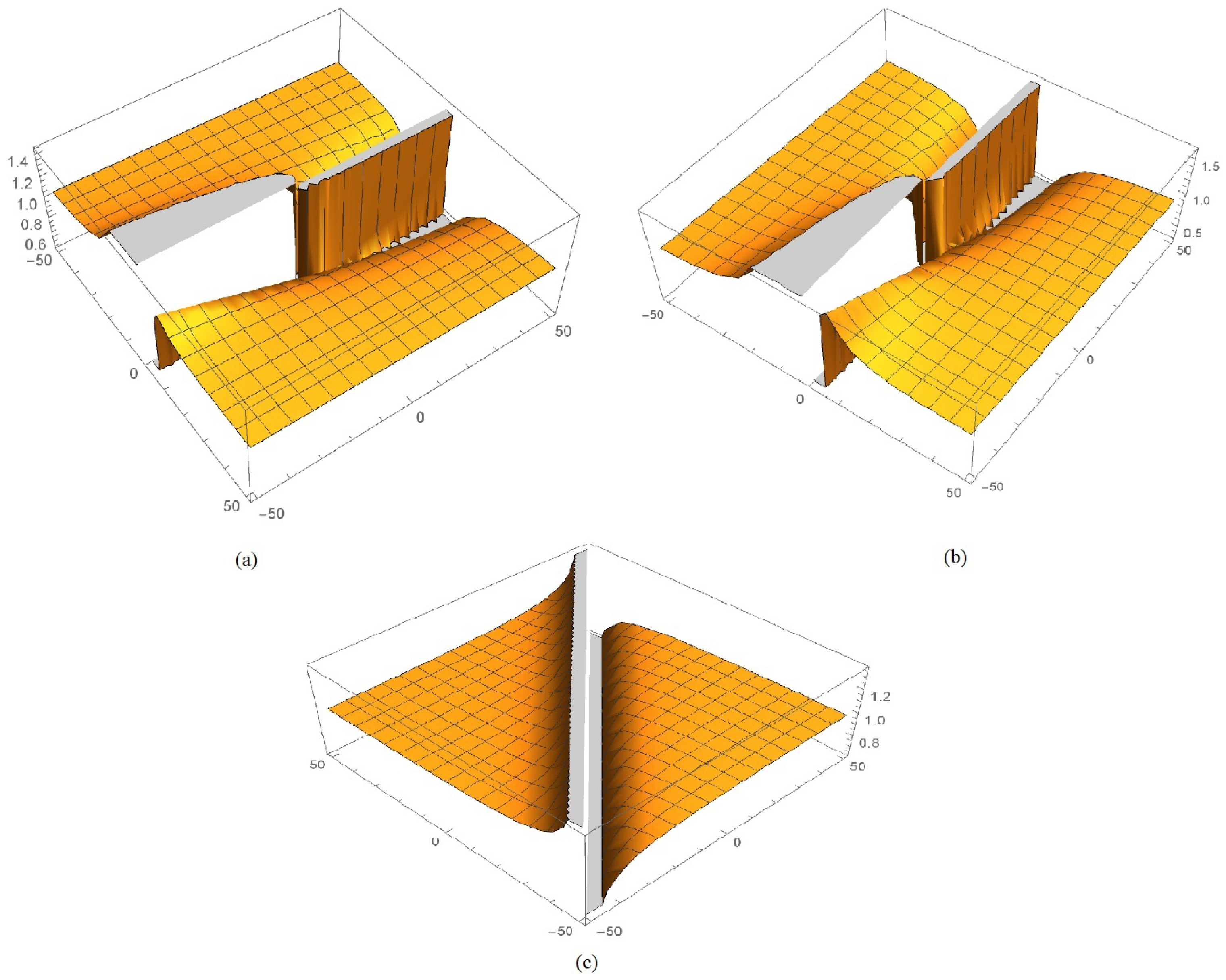
The graphical display of the approximated solution $\mathcal{X}(\overline{\phi },\overline{t})$ is given in Figure 4 for $\alpha =0.5$—$\left(a\right)$, $\alpha =1$—$\left(b\right)$ and the exact solution—$\left(c\right)$, by using the computer software $Mathematic{a}^{TM}$-version 11.1.

Burger’ s equation is the mathematical formulation of fluid flow, viscid/inviscid especially of paints and charcoal etc. It also represents the flow in the air. The solution of Burger’s equation helps us form the paints and design of air vehicles. Then, we gave a representation for the exact solution of Burger’ s equation, studied with the LVI scheme.

Let us consider in the following the time fractional version of non-linear Schrödinger equation, that is the quantum counterpart of Newton’s second law in classical mechanics. It forecast the evolution of a physical system over time, that is, the Schrödinger equation presents the evolution over time of a wave function. This law was postulated by Schrödinger himself in 1925 and published in 1926. It has both linear and non-linear versions.

The standard form of the Schrödinger equation is:

$$i{D}_{\overline{t}}^{\alpha }\mathcal{X}+{\mathcal{X}}_{\overline{\phi }\overline{\phi }}+\gamma {\left|\mathcal{X}\right|}^2\mathcal{X}=0,$$

(17)

where $\gamma$ is a constant (see [17]).

Example 3.

Let us consider the Schrödinger equation with $\gamma =1$,

$$i{D}_{\overline{t}}^{\alpha }\mathcal{X}+{\mathcal{X}}_{\overline{\phi }\overline{\phi }}+{\left|\mathcal{X}\right|}^2\mathcal{X}=0;\mathcal{X}(\overline{\phi },0)=e^{2i\overline{\phi }}.$$

(18)

By implementing the Laplace variational iteration, we get:

$${\mathcal{X}}_{n+1}(\overline{\phi },s)={\mathcal{X}}_n(\overline{\phi },\overline{s})+\mathcal{L}\{\lambda \{i{D}_{\overline{t}}^{\alpha }{\tilde{\mathcal{X}}}_n(\overline{\phi },\overline{s})+\left|{\widetilde{\mathcal{X}{}^2}}_n(\overline{\phi },\overline{s})\right|{\tilde{\mathcal{X}}}_n(\overline{\phi },\overline{s})+\frac{{\partial }^2{\tilde{\mathcal{X}}}_n(\overline{\phi },\overline{s})}{\partial {\overline{\phi }}^2}\}\}.$$

Using optimality conditions we get the following results:

$$\frac{\delta {\tilde{\mathcal{X}}}_{n+1}(\overline{\phi },\overline{s})}{\delta {\tilde{\mathcal{X}}}_n(\overline{\phi },\overline{s})}=0,\delta {\tilde{\mathcal{X}}}_n=0and\lambda =-\frac{\overline{s}+\alpha (1-\overline{s})}{\overline{s}}.$$

Replacing and using inverse Laplace transform we have:

$$\begin{array}{cc}\hfill {\mathcal{X}}_{n+1}(\overline{\phi },\overline{t})& ={\mathcal{X}}_n(\overline{\phi },\overline{t})-{\mathcal{L}}^{-1}\{\frac{\overline{s}+\alpha (1-\overline{s})}{\overline{s}}\mathcal{L}\{i{D}_{\overline{t}}^{\alpha }{\mathcal{X}}_n(\overline{\phi },\overline{s})\hfill \\ \hfill & +|{\mathcal{X}}_n(\overline{\phi },\overline{s}){|}^2{\mathcal{X}}_n(\overline{\phi },\overline{s})+\frac{{\partial }^2{\mathcal{X}}_n(\overline{\phi },\overline{s})}{\partial {\overline{\phi }}^2}\}\}.\hfill \end{array}$$

For $n = 0, 1, 2, \dots$, we get the approximations ${\mathcal{X}}_1, {\mathcal{X}}_2, {\mathcal{X}}_3\dots$ such as,

$${\mathcal{X}}_1(\overline{\phi },\overline{t})=e^{2i\overline{\phi }}-e^{6i\overline{\phi }}(1-\alpha +\overline{t}\alpha ),$$

and

$$\begin{array}{cc}\hfill {\mathcal{X}}_2(\overline{\phi },\overline{t})& =e^{2i\overline{\phi }}-e^{6i\overline{\phi }}(1-\alpha +\overline{t}\alpha )\hfill \\ \hfill & +\frac{1}{4}{\overline{t}}^4{\alpha }^4{e}^{18i\overline{\phi }}-{\overline{t}}^3{\alpha }^3{e}^{14i\overline{\phi }}(1-2e^{4i\overline{\phi }}+2e^{4i\overline{\phi }}\alpha )+\dots ,\hfill \end{array}$$

and so on.

We get the solution in a series form, such as $\mathcal{X}(\overline{\phi },\overline{t})=\underset{i\to \infty }{lim}{\mathcal{X}}_i$, that give the exact solution as $\mathcal{X}(\overline{\phi },\overline{t})=e^{i(2\overline{\phi }-3\overline{t})}$ for $\alpha =1$ (see [17]).

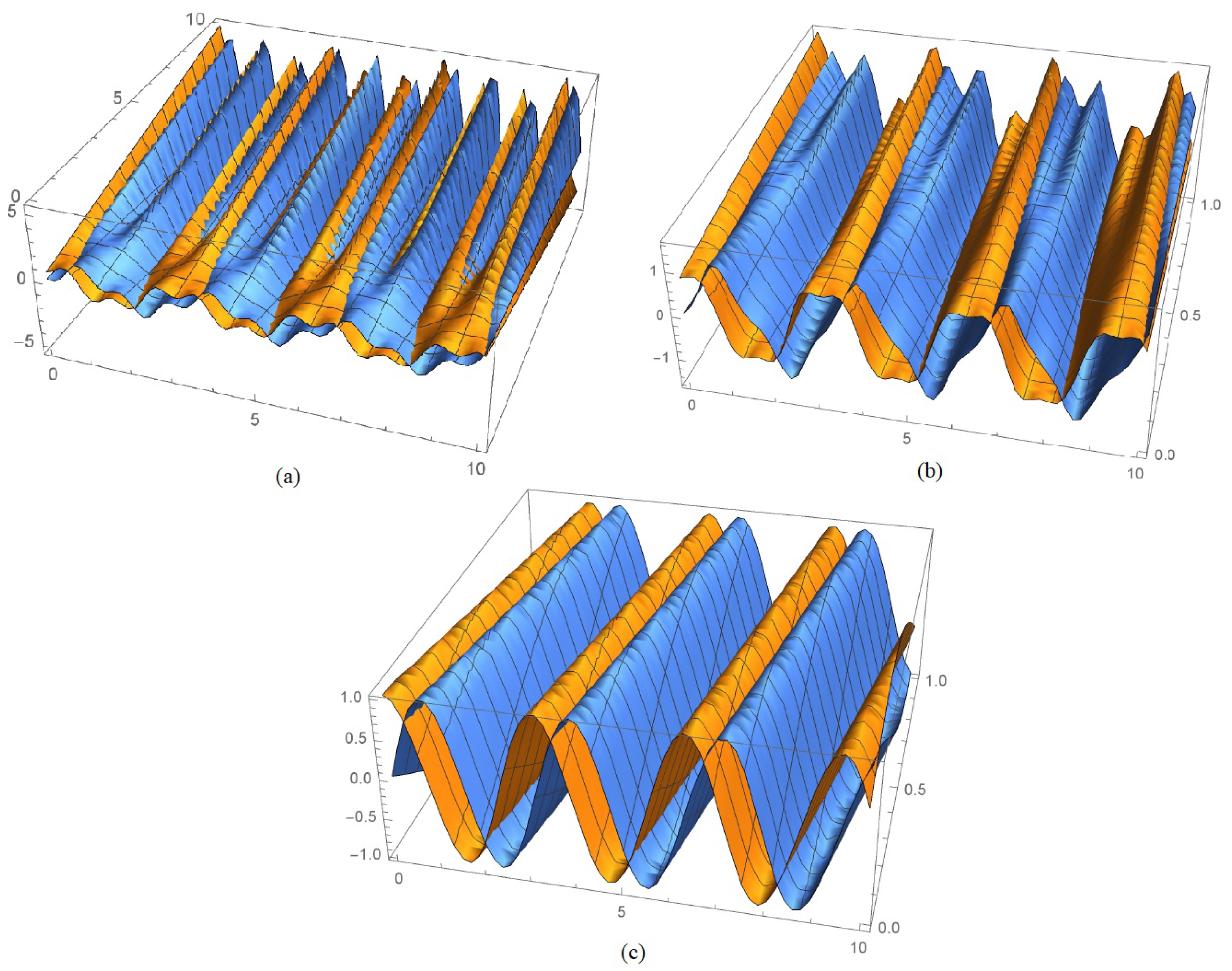
The graphical representation of the approximated solution $\mathcal{X}(\overline{\phi },\overline{t})$ is illustrated in Figure 5 for $\alpha =0.5$—$\left(a\right)$, $\alpha =0.8$—$\left(b\right)$ and the exact solution—$\left(c\right)$, with the computer software $Mathematic{a}^{TM}$-version 11.1, in the following.

The solution of the Schrodinger equation describes the behavior of a particle in the deep well, the probability of its motion, position and the wave associated with it. We gave above the 3D graphic interpretation of such a solution, obtained by our proposed LVI analytic scheme.

Remark 1.

As a remark concerning LVI on nonlinear fractional order partial differential equations is the existence of the approximations of the solution ${\mathcal{X}}_1,{\mathcal{X}}_2,{\mathcal{X}}_3\dots$. From Section 3 it is easy to conclude that these approximations of the solution are similar to the iterations of a sequence of successive approximations which is convergent to a fixed point. Then, we get a strong connection between the proposed scheme and the fixed point theory. It would be very interesting to check in which conditions we get a fixed point for this type of approximation.

5. Discussion and Conclusions

In this work, we proposed a new semi analytic scheme in order to solve non-linear fractional order partial differential equations. By solving some non-linear fractional order partial differential equations, we proved that the proposed scheme converges faster than the existing ones in the literature and is a more reliable technique.

Though there are many methods to solve nonlinear equations, either ODEs, PDEs or FOPDEs, such as the Adomian decomposition method, variational iteration method, homotopy perturbation method etc. (see [17,24]), all these techniques have some limitations, for example:

• The calculation of Adomian polynomials in the Adomian decomposition method is not an easy task;
• In the variational iteration method, Lagrange’s multiplier is very difficult to calculate;
• Similarly, the calculation of He’s polynomials in homotopy analysis as well as in the homotopy perturbation method is a time consuming task.

These difficulties are not faced in the proposed LVI; one has to find neither Adomian polynomials, He’s polynomials nor Lagrange’s multiplier etc. Our proposed scheme improves the time and the algorithm of these previous iteration methods. Then, any researcher with little knowledge of the software $Mathematic{a}^{TM}$, may work with the proposed scheme, LVI.

Concerning the figures of all three examples given here, the first two figures are of the first iteration for $\alpha =0.5$, $\alpha =0.8$ or $\alpha =1$ and the third figure is of the exact solution. The aim of the diagrams is to show the convergence of the proposed LVI analytic scheme towards the exact solution. The difference between the figures of the approximated solution and that of the exact solution is because we take just the first iteration and draw diagrams; if we use the second or third iterations, keeping the value of $\alpha$ small, the difference between the figures for the approximated solution and that of the exact solution will be negligible, showing the exactness of the proposed scheme.

The accuracy of the results of the LVI scheme is represented in the 3D-graphical displays. We also put in evidence a relationship between the approximations ${\mathcal{X}}_1,{\mathcal{X}}_2,{\mathcal{X}}_3\dots$ of the solution and the iterations of the sequence of successive approximations used in the proof of the existence of a fixed point. The main advantage is that the proposed scheme streamlines the computational processes and can be used efficiently for nonlinear dynamical systems analysis based on softwares as $Mathematic{a}^{TM}$, $Matla{b}^{TM}$ and $Mapl{e}^{TM}$ etc.

References

1. De Jager, E.M. On the origin of the Korteweg–de Vries equation. arXiv 2006, arXiv:math/0602661. [Google Scholar]
2. Grunert, K.; Teschl, G. Long-time asymptotics for the Korteweg–de Vries equation via nonlinear steepest descent. Math. Phys. Anal. Geom. 2009, 12, 287–324. [Google Scholar] [CrossRef] [Green Version]
3. Halliday, D.; Resnick, R.; Merrill, J. Fundamentals of Physics; Wiley: New York, NY, USA, 1981; Volume 9. [Google Scholar]
4. Hicdurmaz, B. Finite difference schemes for time-fractional Schrödinger equations via fractional linear multistep method. Int. J. Comput. Math. 2021, 98, 1561–1573. [Google Scholar] [CrossRef]
5. Serway, R.A.; Moses, C.J.; Moyer, C.A. Modern Physics; Cengage Learning: Boston, MA, USA, 2004. [Google Scholar]
6. Lin, J.; Xu, Y.; Zhang, Y. Simulation of linear and nonlinear advection–diffusion–reaction problems by a novel localized scheme. Appl. Math. Lett. 2020, 99, 106005. [Google Scholar] [CrossRef]
7. Saleh, R.; Mabrouk, S.M.; Wazwaz, A.M. The singular manifold method for a class of fractional-order diffusion equations. Waves Random Complex Media 2021, 1–12. [Google Scholar] [CrossRef]
8. Akram, T.; Abbas, M.; Riaz, M.B.; Ismail, A.I.; Ali, N.M. An efficient numerical technique for solving time fractional Burgers equation. Alex. Eng. J. 2020, 59, 2201–2220. [Google Scholar] [CrossRef]
9. Lodhi, S.; Manzar, M.A.; Raja, M.A.Z. Fractional neural network models for nonlinear Riccati systems. Neural Comput. Appl. 2019, 31, 359–378. [Google Scholar] [CrossRef]
10. Vijayakumar, V.; Ravichandran, C.; Nisar, K.S.; Kucche, K.D. New discussion on approximate controllability results for fractional Sobolev type Volterra-Fredholm integro-differential systems of order 1 < r < 2. Numer. Methods Partial Differ. Equ. 2021, 1–19. [Google Scholar] [CrossRef]
11. Hietarinta, J. Introduction to the Hirota bilinear method. In Integrability of Nonlinear Systems; Springer: Berlin/Heidelberg, Germany, 1997; pp. 95–103. [Google Scholar]
12. Zhang, Z.; Li, B.; Chen, J.; Guo, Q. Construction of higher-order smooth positons and breather positons via Hirota’s bilinear method. Nonlinear Dyn. 2021, 105, 2611–2618. [Google Scholar] [CrossRef]
13. Davies, B. Integral Transforms and Their Applications; Springer: Berlin/Heidelberg, Germany, 2012; Volume 41. [Google Scholar]
14. Podlubny, I. The Laplace transform method for linear differential equations of the fractional order. arXiv 2006, arXiv:functan/9710005. [Google Scholar]
15. Anjum, N.; He, J.H. Laplace transform: Making the variational iteration method easier. Appl. Math. Lett. 2019, 92, 134–138. [Google Scholar] [CrossRef]
16. He, J.H. Variational iteration method-a kind of non-linear analytical technique: Some examples. Int. J. Nonlinear Mech. 1999, 34, 699–708. [Google Scholar] [CrossRef]
17. Wazwaz, A.M. Partial Differential Equations and Solitary Waves Theory; Springer: Berlin/Heidelberg, Germany, 2010. [Google Scholar]
18. Gil, A.; Segura, J.; Temme, N.M. Numerical Methods for Special Functions; Cambridge University Press: Cambridge, UK, 2007; Volume 99. [Google Scholar]
19. Kanwal, A.; Phang, C.; Loh, J.R. New collocation scheme for solving fractional partial differential equations. Hacet. J. Math. Stat. 2020, 49, 1107–1125. [Google Scholar] [CrossRef] [Green Version]
20. Khader, M.M.; Saad, K.M.; Hammouch, Z.; Baleanu, D. A spectral collocation method for solving fractional KdV and KdV-Burgers equations with non-singular kernel derivatives. Appl. Numer. Math. 2021, 161, 137–146. [Google Scholar] [CrossRef]
21. Loh, J.R.; Isah, A.; Phang, C.; Toh, Y.T. On the new properties of Caputo-Fabrizio operator and its application in deriving shifted Legendre operational matrix. Appl. Numer. Math. 2018, 132, 138–153. [Google Scholar] [CrossRef]
22. Yavuz, M.; Sulaiman, T.A.; Usta, F.; Bulut, H. Analysis and numerical computations of the fractional regularized long-wave equation with damping term. Math. Methods Appl. Sci. 2021, 44, 7538–7555. [Google Scholar] [CrossRef]
23. Arshad, M.S.; Iqbal, J. Semi-Analytical Solutions of Time-Fractional KdV and Modified KdV Equations. Sci. Inq. Rev. 2019, 3, 47–59. [Google Scholar] [CrossRef]
24. Arshad, S.; Sohail, A.; Maqbool, K. Nonlinear shallow water waves: A fractional order approach. Alex. Eng. J. 2016, 55, 525–532. [Google Scholar] [CrossRef] [Green Version]
25. Iqbal, J.; Shabbir, K.; Guran, L. Semianalytical Solutions of Some Nonlinear-Time Fractional Models Using Variational Iteration Laplace Transform Method. J. Funct. Spaces 2021, 2021, 8345682. [Google Scholar] [CrossRef]
26. Karakoc, S.B.G.; Ali, K.K. Theoretical and computational structures on solitary wave solutions of Benjamin Bona Mahony-Burgers equation. Tbil. Math. J. 2021, 14, 33–50. [Google Scholar] [CrossRef]
27. Yavuz, M.; Sulaiman, T.A.; Yusuf, A.; Abdeljawad, T. The Schrödinger-KdV equation of fractional order with Mittag-Leffler nonsingular kernel. Alex. Eng. J. 2021, 60, 2715–2724. [Google Scholar] [CrossRef]
28. Zhang, J.; Wang, J.; Zhou, Y. Numerical analysis for time-fractional Schrödinger equation on two space dimensions. Adv. Differ. Equ. 2020, 53, 1–16. [Google Scholar] [CrossRef] [PubMed] [Green Version]
29. Caputo, M.; Fabrizio, M. On the singular kernels for fractional derivatives. Some applications to partial differential equations. Progr. Fract. Differ. Appl. 2021, 7, 1–4. [Google Scholar]
30. Caputo, M.; Fabrizio, M. A new definition of fractional derivative without singular kernel. Progr. Fract. Differ. Appl. 2015, 1, 1–13. [Google Scholar]
31. Ain, Q.T.; Anjum, N.; Din, A.; Zeb, A.; Djilali, S.; Khan, Z.A. On the analysis of Caputo fractional order dynamics of Middle East Lungs Coronavirus (MERS-CoV) model. Alex. Eng. J. 2022, 61, 5123–5131. [Google Scholar] [CrossRef]
32. Dong, Y.; Tang, X.; Yuan, Y. Principled reward shaping for reinforcement learning via Lyapunov stability theory. Neurocomputing 2020, 393, 83–90. [Google Scholar] [CrossRef]
33. Li, L.; Chen, W. Exponential stability analysis of quaternion-valued neural networks with proportional delays and linear threshold neurons: Continuous-time and discrete-time cases. Neurocomputing 2020, 381, 152–166. [Google Scholar] [CrossRef]
34. Yang, X.; Li, C.; Huang, T.; Song, Q. Mittag-Leffler stability analysis of nonlinear fractional-order systems with impulses. Appl. Math. Comput. 2017, 293, 416–422. [Google Scholar] [CrossRef]
35. Ali, A.; Mahariq, I.; Shah, K.; Abdeljawad, T.; Al-Sheikh, B. Stability analysis of initial value problem of pantograph-type implicit fractional differential equations with impulsive conditions. Adv. Differ. Equ. 2021, 1, 1–17. [Google Scholar] [CrossRef]
36. Kreyszig, E. Introductory Functional Analysis with Applications; John Wiley Sons: Hoboken, NJ, USA, 1991; Volume 17. [Google Scholar]
Figure 1. The rectangle R.
Fractalfract 06 00393 g001
Figure 2. Graphical representation of | S ( t ¯ , X ) | c .
Fractalfract 06 00393 g002
Figure 3. Three dimensional (3D) display of X ( φ ¯ , t ¯ ) for α = 0.5 —(a), α = 1 —(b) and for the exact solution—(c).
Fractalfract 06 00393 g003
Figure 4. Three dimensional (3D) display of X ( φ ¯ , t ¯ ) for α = 0.5 —(a), α = 1 —(b) and the exact solution—(c).
Fractalfract 06 00393 g004
Figure 5. Three dimensional (3D) display of X ( φ ¯ , t ¯ ) for α = 0.5 —(a), α = 0.8 —(b) and the exact solution—(c).
Fractalfract 06 00393 g005
Publisher’s Note: MDPI stays neutral with regard to jurisdictional claims in published maps and institutional affiliations.