Abstract
In this paper, circuit implementation and anti-synchronization are studied in coupled nonidentical fractional-order chaotic systems where a fractance module is introduced to approximate the fractional derivative. Based on the open-plus-closed-loop control, a nonlinear coupling strategy is designed to realize the anti-synchronization in the fractional-order Rucklidge chaotic systems and proved by the stability theory of fractional-order differential equations. In addition, using the frequency-domain approximation and circuit theory in the Laplace domain, the corresponding electronic circuit experiments are performed for both uncoupled and coupled fractional-order Rucklidge systems. Finally, our circuit implementation including the fractance module may provide an effective method for generating chaotic encrypted signals, which could be applied to secure communication and data encryption.
1. Introduction
Presently, synchronization of fractional-order dynamical systems has been widely investigated due to its importance in a variety of fields including voice encryption [1], image encryption [2], and secure communication [3]. There are many types of synchronization in fractional-order chaotic systems, such as complete synchronization [4], anti-synchronization [5], generalized synchronization [6], and so on. In these architectures of various synchronization phenomena, the master-slave or drive-response topology comes from the seminal work of Pecora-Carroll. Coupling two nonlinear systems with higher-dimension has rich complex dynamics. Such a coupling is similar to the transmitter-receiver system of data communication. For example, two synchronized fractional-order chaotic oscillators are adapted to design a transmitter-receiver topology implemented on the FPGAs [7]. In this case, the masking of images are effectively performed by the fractional-order chaotic attractors.
Circuit realization and chaos control of fractional-order systems have attracted considerable attention. For example, chaos control and circuit simulation of a novel 3D finance chaotic system is established using the adaptive control method [8]. Design of fractional-order hyper-chaotic systems with maximum number of positive Lyapunov exponent and their anti-synchronization are also depicted by adaptive control [9]. Among the current control methods, the open-plus-closed-loop (OPCL) control is a general and systematic approach for integer-order chaotic dynamical systems [10,11,12,13,14], which facilitates the targeted synchronization of coupled chaotic systems. In the synchronization regimes, it is possible to amplify or attenuate a chaotic attractor with respect to other chaotic attractors [11]. For the practical applications, a general formulation of the OPCL coupling for synchronization is presented in chaotic oscillators for unidirectional and bidirectional modes [12,13,14]. This opens a new topic how to extend the OPCL technology to fractional-order counterparts.
The OPCL coupling is a physically realizable scheme that can provide the modified projective synchronization of different fractional-order chaotic systems under the parameter mismatch [15]. Inverse synchronization of coupled fractional-order systems has been shown numerically by the OPCL method [16]. Furthermore, the OPCL coupling scheme is also applied to a limit cycle system, a chaotic system, and a hyper-chaotic system [17]. In the current OPCL coupling schemes for the fractional-order chaotic oscillators, there are many advantages of the OPCL control. It provides synchronization in all systems without restrictions on the symmetry class of a dynamical system. It also achieves the stable amplification or attenuation in coupled identical or nonidentical chaotic systems. Furthermore, it presents a physical feasible method to obtain various types of synchronization [18,19,20]. However, few results involve both the circuit implementation and anti-synchronization of fractional-order chaotic systems.
It is known that there are many circuit modules, such as resistor-inductor circuit (RL), oscillation of logic circuit (LC), resistor-capacitance circuit (RC), and relay logic circuit (RLC). Recently, the analytical solutions of the RL, LC, RC, and RLC electrical circuits described by the Caputo or left generalized fractional derivative have been demonstrated and proved theoretically [21]. Based on Laplace transform and inverse Laplace transform, these solutions are expressed by the generalized Mittag–Leffler function. Based on the real RC unit, coupled integer-order and fractional-order Sprott systems are achieved by a transition from complete synchronization to anti-synchronization (or vice versa) via the unidirectional OPCL coupling [5]. Its experimental mix circuits are redesigned by two types of fractance, i.e., the chain-type and tree-type. Inspired by the above discussions, a different circuit module is reconstructed for the fractance, whose topology is composed of one RC parallel circuit and two RC series circuit in the form of parallel. Then, this parallel configuration with an operational amplifier is chosen to accomplish the fractional-order derivative in the circuit implementation.
The rest of this paper is as follows. Section 2 presents the fractional-order Rucklidge system with commensurate order and its electronic circuit. The fractional-order differential operator in our electronic implementations is composed of three parallel circuits. In Section 3, anti-synchronization of coupled nonidentical fractional-order Rucklidge systems based on open-loop design is proved correctness theoretically. A physical realization of this drive-response circuit system is presented by National Instruments (NI) Multisim Software. Section 4 includes the conclusions.
2. Fractional-Order Rucklidge Systems and Its Circuit Realization
Fractional calculus possesses definitions that come from the definitions of ordinary derivatives. Some of the existing definitions for fractional derivatives are described in Ref. [22]. The th-order Caputo fractional derivative of function with respect to t and the terminal value 0 is given by
where , i.e., m is the first integer which is no less than , and is the Gamma function, . The Laplace transform of the Caputo fractional derivative is given as follows: .
For the zero initial conditions, the fractional integral operator of order “” can be represented by the transfer function in the frequency domain. It is known that the standard definition of fractional differ-integral does not allow direct engineering applications and circuit implementation of the fractional operators. An efficient scheme to circumvent this problem is to approximate fractional operators by using standard integer-order operators.
Based on the idea of parallel integer-order operators, a different circuit unit is reconstructed in this paper to accomplish the approximations of transfer function (fractance ), whose circuit’s topology is composed of one RC parallel circuit and two RC series circuit in parallel form. This configuration of circuit unit is unlike the recent tree-type or chain-type topology of fractance () [5]. Under the requirements of an approximation technique for the fractance, our focus is on the commensurate-order fractional-order systems. In addition, the two-scroll fractional-order Rucklidge system with commensurate order is considered in this paper.
Moreover, the stability theorem for the canonical fractional differential equations with a commensurate order should be given first.
Lemma 1
([23,24]). The following autonomous system:
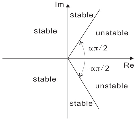
with , and , is asymptotically stable if and only if |arg(λ)|> is satisfied for all eigenvalues (λ) of matrix A. Furthermore, this system is stable if and only if |arg(λ)| ≥ is satisfied for all the eigenvalues (λ) of matrix A with those critical eigenvalues satisfying |arg(λ)| = having geometric multiplicity of one. The geometric multiplicity of an eigenvalue λ of the matrix A is the dimension of the subspace of vectors v satisfying . The stable and unstable regions for are shown in Figure 1.
Figure 1.
Stable region of linear fractional-order system (2).
2.1. Fractional-Order Rucklidge Systems
The fractional-order Rucklidge system was introduced in of the following form [25], which is given by
where the commensurate fractional order is subject to , and and are constant system parameters. For a typical set of parameter values: (,) = (2,6.7), the fixed points and their corresponding eigenvalues are Hence, are saddle points of index 2. According to Refs. [23,24], the necessary condition for the fractional-order Rucklidge system with the commensurate order to remain chaotic is
2.2. Circuit Realization of Commensurate Fractional-Order Rucklidge Systems
In this section, an electronic circuit achieving a fractional-order Rucklidge system with order 2.85 is designed, where two RC series circuits and one RC parallel circuit are connected in parallel as shown in Figure 2. According to the circuitry theory in the Laplace domain, the corresponding circuit unit between A and B in Figure 2 can realize the approximations of fractance with [26]. Here, the transfer function approximation method and its Laplace domain expression are given, respectively, as follows:
where is a unit parameter. Let and . By comparing the constant coefficients in numerator and denominator of Equation (4) with unknown parameters in numerator and denominator of Equation (5), it obtains the following parameter values of resistances and capacitances: = 694.6 M, = 32.82 M, = 0.326 M, = 0.779 F, = 0.2699 F, = 0.2133 F.
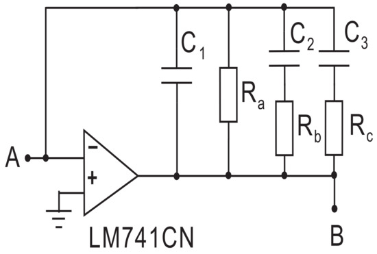
Figure 2.
The circuit unit to realize .
On the other hand, a circuit is redesigned to realize the 2.85-order Rucklidge system as shown in Figure 3, where AD633 is the multiplier with an output coefficient of 0.1 and LM741CN is the operational amplifier. In this electronic circuit, the three state variables and z are obtained from the terminal outputs of U3, U5 and U7, respectively.
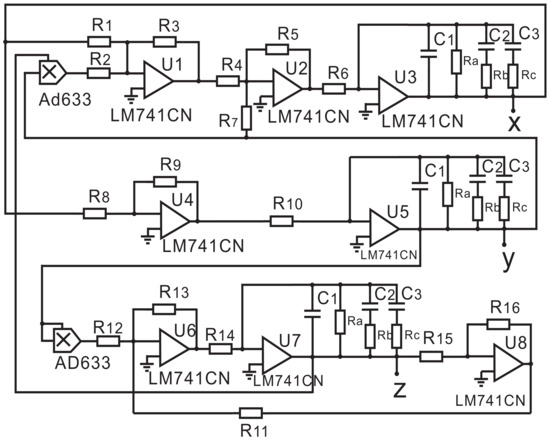
Figure 3.
2.85-order Rucklidge circuit system.
From the circuit design shown in Figure 3, we obtain the 2.85-order Rucklidge system equation in the Laplace domain as follows:
The resistance parameters can be obtained by comparing the corresponding coefficients of the Laplace transform domain system of the following time-domain system (7) and the above frequency domain system (6). Then, it yields = 500 , = = = = = = = = = 100 , = = = = = 1 k, = 149.25 . Please note that the values of these resistance and capacitance parameters are not unique.
Based on the inverse Laplace transform method and , the time-domain system is given by
Here the new time variable () for the fast circuit experiment results from the chosen values of resistances . Using the Multisim to simulate system (7), its two-scroll chaotic trajectories are obtained. To show a clear diagram, the real circuit data displayed on the Multisim high-frequency oscilloscope are saved and drawn in Figure 4 on the Matlab.
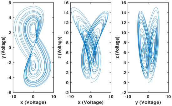
Figure 4.
Chaotic oscillator of 2.85-order Rucklidge system by Multisim.
3. Anti-Synchronization of Coupled Nonidentical Fractional-Order Rucklidge Systems
3.1. Open-Loop and Closed-Loop Design
In this section, stable anti-synchronization of two coupled nonidentical fractional-order chaotic systems is achieved by designing an open-loop and closed-loop method. A fraction-order drive system is defined by
where and contains the mismatch terms.
The model of the fractional-order chaotic oscillator with parameters is assumed to be known. It drives another fractional-order chaotic oscillator , to achieve a desired goal dynamics , i.e., the anti-synchronization. Here, the subscripts d and r stand for the drive (or master) and the response (or slave) systems, respectively. By the coupling, the response system reads as
where the coupling function is defined as the sum of Huble’s open-loop interaction () and a linear closed-loop interaction () [11], i.e.,
and
where is the Jacobian matrix, and is an constant control matrix which is not necessarily a Hurwitz matrix [8,15].
To prove the local stability of anti-synchronization, the Taylor series expansion around the goal trajectory is
The fractional-order error system is locally asymptotically stable if all the eigenvalues () of the matrix K satisfy the following condition: , which means that the anti-synchronization happens.
3.2. OPCL Nonlinear Control for Fractional-Order Rucklidge System
In this subsection, an example of coupled fractional-order Rucklidge chaotic systems with mismatch parameters is studied. The mismatch 2.85-order Rucklidge system is taken as a driver:
Let and , then the Jacobian matrix of f is
The open-loop design and closed-loop design are designed in the form below:
and
The control matrix K is
Finally, the response system is given by
The drive and response systems are chaotic before the coupling for the parameters: , , , [25]. How to choose the coefficients , and in Equation (19) becomes an important key for the OPCL control. When the parameters , and are chosen, the corresponding eigenvalues of are , , which do not satisfy the condition of Hurwitz matrix. However, these eigenvalues meet the condition shown in Lemma 1, i.e., ) > . Therefore, the local stable chaotic anti-synchronization between the drive system (14) and response system (19) is achieved. To verify the effectiveness of the OPCL control and approximation of fractance, the experimental validation in the following subsection is applied.
3.3. Circuit Implementation
A physical realization of the coupled nonidentical fractional-order Rucklidge systems (14) and (19) is presented in electronic workbench Multisim. Figure 5 shows the nonlinear coupled circuit. Here, the electronic circuit unit with resistances R-R and capacitances U1-U3 can realize the 0.95-order operator as shown in Section 2. The Op-Amp U1-U8 (U9-U16) with resistances R-R (R-R) represent the driver system 1 (response system 2). Using U17-U21 and resistances R-R, the OPCL nonlinear coupling is designed, and the continuity between the driver system 1, OPCL nonlinear coupling, and response system 2 is maintained via the terminals (1A-1A, 1B-1B and 2A-2A, 2B-2B, 2C-2C, 2D-2D).
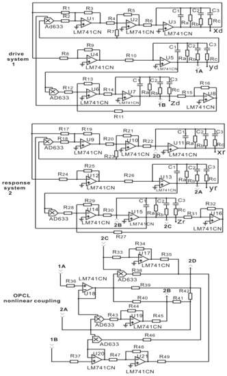
Figure 5.
Coupled 2.85-order Rucklidge circuit. System 1 drives the response system 2 by OPCL nonlinear coupling. Please note that 1% tolerance of component values are allowed.
The practical values of the resistance and capacitances of the drive and response systems are described in Section 2, and the values for OPCL nonlinear coupling unit are chosen as followings: R, R, R, R, R, R, R, R each equals 1 k; R, R, R, R each equals 100 ; R = R = 1 M; R = R = 781.25 ; R = 500 . These coefficients are obtained from the Laplace domain of the six-dimension drive-response systems.
On the other hand, the results of circuit simulation are effective because Multisim software is based on the actual circuit components, and its simulation results should be basically consistent with those of the actual circuit experiment. Please note that the anti-synchronization process displayed on the high-frequency oscilloscope of Multisim is saved and shown in Figure 6 on the Matlab. From Figure 6, it is seen that the anti-synchronization happens. To verify the circuit validation, the time-domain numerical method is depicted in the next subsection.
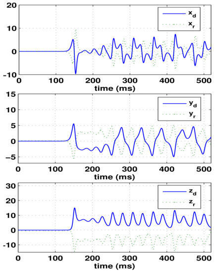
Figure 6.
Observed state variables for the drive system () and its response system () evolution with time (ms) on the electronic workbench Multisim.
3.4. Time-Domain Numerical Methods
There are many numerical algorithms for the fractional-order chaotic systems in the Caputo sense [27,28]. The Adams-Bashforth-Moulton algorithm based on the predictor-corrector scheme was proposed for the fractional-order chaotic systems [28]. A detailed description of the time-domain numerical method is depicted as follows.
The fractional differential equation
is equivalent to the Volterra integral equation, that is,
Here, the approximation error is given by
where .
Then, the time-domain coupled nonidentical fractional-order Rucklidge systems with the OPCL control are
where the parameters are , , , , , , .
Based on this numerical method, the anti-synchronization process is shown in Figure 7, which is consistent with the circuit’s results shown in Figure 6.
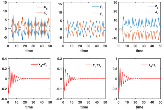
Figure 7.
Anti-synchronization of coupled nonidentical 2.85-order Rucklidge systems.
4. Conclusions
In the present study, the anti-synchronization and circuit implementation of mismatched fractional-order chaotic systems based on open-loop and closed-loop nonlinear control is investigated. For the commensurate fractional Rucklidge chaotic system, an electronic circuit is implemented by NI Multisim software, which includes the modular circuit implementation of the fractance. The reconstructed fractance module circuit is composed of three circuits in parallel, one RC series circuit, another RC series circuit, and a third RC parallel circuit. The parameter values of the resistive and capacitive devices in the fractance module circuit are obtained from the asymptotic approximation of the transfer function. The designed circuit implementation and numerical simulations both prove that the anti-synchronization happens in the Rucklidge system with the OPCL control.
In future work, a transmitter-receiver on the basis of the drive-response system is reconstructed, which could be used for chaotic encryption. For example, the chaotic signal of the fractional drive system signal is used to encrypt the transmitted image signal (e.g., multiplication or addition), and the receiver uses the anti-synchronization method to recover the original signal.
Author Contributions
Y.Z., P.L. and W.S. contributed to the conceptualization and methodology of the study. Y.Z., P.L. and W.S. performed the formal analysis and investigation. Y.Z. and W.S. wrote the manuscript. Y.Z., P.L. and W.S. did the data collection and analysis. All authors have read and agreed to the published version of the manuscript.
Funding
This work was financially sponsored by the National Natural Science Foundation of China (No. 11804300), and the Science Foundation of Zhejiang Sci-Tech University (ZSTU) under Grant No. 17062062-Y.
Institutional Review Board Statement
Not applicable.
Informed Consent Statement
Not applicable.
Data Availability Statement
Not applicable.
Conflicts of Interest
The authors declare no conflict of interest.
References
- Jahanshahi, H.; Yousefpour, A.; Munoz Pacheco, J.M.; Kacar, S.; Pham, V.-T.; Alsaadi, F.E. A new fractional-order hyperchaotic memristor oscillator: Dynamic analysis, robust adaptive synchronization, and its application to voice encryption. Appl. Math. Comput. 2020, 383, 125310. [Google Scholar] [CrossRef]
- Sayed, W.S.; Radwan, A.G. Generalized switched synchronization and dependent image encryption using dynamically rotating fractional-order chaotic systems. AEU-Int. J. Electron. Commun. 2020, 123, 153268. [Google Scholar] [CrossRef]
- Khan, A.; Jahanzaib, L.S.; Trikha, P. Secure communication: Using parallel synchronization technique on novel fractional order chaotic system. IFAC-Papers OnLine 2020, 53, 307–312. [Google Scholar] [CrossRef]
- Qi, F.; Qu, J.; Chai, Y.; Chen, L.; Lopes, A.M. Synchronization of incommensurate fractional-order chaotic systems based on linear feedback control. Fractal Fract. 2022, 6, 221. [Google Scholar] [CrossRef]
- Adedayo, O.A. OPCL coupling of mixed integer-fractional order oscillators: Tree and chain implementation. Phys. Scr. 2021, 96, 125270. [Google Scholar]
- Martínez-Fuentes, O.; Montesinos-García, J.J.; Gómez-Aguilar, J.F. Generalized synchronization of commensurate fractional-order chaotic systems: Applications in secure information transmission. Digit. Signal Process. 2022, 126, 103494. [Google Scholar] [CrossRef]
- Tlelo-Cuautle, E.; Dalia Pano-Azucena, A.; Guillén-Fernández, O.; Silva-Juárez, A. Synchronization and Applications of Fractional-Order Chaotic Systems. In Analog/Digital Implementation of Fractional Order Chaotic Circuits and Applications; Springer: Cham, Switzerland, 2020; pp. 175–201. [Google Scholar]
- Vaidyanathan, S.; Volos, C.K.; Tacha, O.I.; Kyprianidis, I.; Stouboulos, I.; Pham, V.T. Analysis, control and circuit simulation of a novel 3-D finance chaotic system. In Advances and Applications in Chaotic Systems; Springer: Cham, Switzerland, 2016; pp. 495–512. [Google Scholar]
- Borah, M.; Roy, B.K. Design of fractional-order hyperchaotic systems with maximum number of positive lyapunov exponents and their antisynchronisation using adaptive control. Int. J. Control 2016, 91, 2615–2630. [Google Scholar] [CrossRef]
- El-Sayed, A.; Nour, H.; Elsaid, A.; Matouk, A.; Elsonbaty, A. Dynamical behaviors, circuit realization, chaos control, and synchronization of a new fractional order hyperchaotic system. Appl. Math. Model. 2016, 40, 3516–3534. [Google Scholar] [CrossRef]
- Grosu, I.; Banerjee, R.; Roy, P.K.; Dana, S.K. Design of coupling for synchronization of chaotic oscillators. Phys. Rev. E 2009, 80, 016212. [Google Scholar] [CrossRef]
- Padmanaban, E.; Hens, C.; Dana, S.K. Engineering synchronization of chaotic oscillators using controller based coupling design. Chaos 2011, 21, 013110. [Google Scholar] [CrossRef]
- Roy, P.K.; Hens, C.; Grosu, I.; Dana, S.K. Engineering generalized synchronization in chaotic oscillators. Chaos 2011, 21, 013106. [Google Scholar] [CrossRef]
- Bhowmick, S.K.; Ghosh, D. Targeting engineering synchronization in chaotic systems. Int. J. Mod. Phys. C 2016, 27, 1650006. [Google Scholar] [CrossRef]
- Liu, H.; Zhu, Z.; Yu, H.; Zhu, Q. Modified projective synchronization between different fractional-order systems based on open-plus-closed-loop control and its application in image encryption. Math. Probl. Eng. 2014, 2014, 567898. [Google Scholar] [CrossRef]
- Wang, J.W.; Zeng, L.; Ma, Q.H. Inverse synchronization of coupled fractional-order systems through open-plus-closed-loop control. Pramana-J. Phys. 2011, 76, 385–396. [Google Scholar] [CrossRef]
- Wang, J.W.; Zhang, Y.B. Synchronization in coupled nonidentical incommensurate fractional-order systems. Phys. Lett. A 2009, 374, 202–207. [Google Scholar] [CrossRef]
- Banerjee, R.; Padmanaban, E.; Dana, S.K. Control of partial synchronization in chaotic oscillators. Pramana-J. Phys. 2015, 84, 203–215. [Google Scholar] [CrossRef]
- Bhowmick, S.K.; Bera, B.K.; Ghosh, D. Generalized counter-rotating oscillators: Mixed synchronization. Commun. Nonlinear Sci. Numer. Simul. 2015, 22, 692–701. [Google Scholar] [CrossRef][Green Version]
- Chen, X.; Cao, J.; Qiu, J.; Yang, C. Transmission synchronization control of multiple non-identical coupled chaotic systems. IEEE Trans. Neural Netw. Learn. Syst. 2016, 26, 1115–1120. [Google Scholar]
- Sene, N.; G’omez-Aguilar, J.F. Analytical solutions of electrical circuits considering certain generalized fractional derivatives. Eur. Phys. J. Plus 2019, 134, 260. [Google Scholar] [CrossRef]
- Podlubny, I. Fractional Differential Equations: An Introduction to Fractional Derivatives, Fractional Differential Equations, to Methods of Their Solution and Some of Their Applications, 1st ed.; Academic Press: Cambridge, MA, USA, 1999; p. 62. [Google Scholar]
- Matignon, D. Stability results for fractional differential equations with applications to control processing. In Proceedings of the Computational Engineering in Systems and Application Multi-Conference, IMACS, Lille, France, 9–12 July 1996; pp. 963–968. [Google Scholar]
- Bahatdin, D. Stability analysis of an incommensurate fractional-order SIR model. Math. Model. Numer. Simul. Appl. 2021, 1, 44–55. [Google Scholar]
- Zhang, Y.B.; Zhou, T.S. Three schemes to synchronize chaotic fractional-order Rucklidge systems. Int. J. Mod. Phys. B 2007, 21, 2033–2044. [Google Scholar] [CrossRef]
- Zhang, R.X.; Yang, S.P. Chaos in fractional-order generalized Lorenz system and its synchronization circuit simulation. Chin. Phys. B 2009, 18, 03295. [Google Scholar]
- Hammouch, Z.; Yavuz, M.; Özdemir, N. Numerical solutions and synchronization of a variable-order fractional chaotic system. Math. Model. Numer. Simul. Appl. 2021, 1, 11–23. [Google Scholar] [CrossRef]
- Diethelm, K.; Ford, N.J.; Freed, A.D. Detailed error analysis for a fractional Adams method. Numer. Algorithms 2004, 36, 31–52. [Google Scholar] [CrossRef]


Publisher’s Note: MDPI stays neutral with regard to jurisdictional claims in published maps and institutional affiliations. |
© 2022 by the authors. Licensee MDPI, Basel, Switzerland. This article is an open access article distributed under the terms and conditions of the Creative Commons Attribution (CC BY) license (https://creativecommons.org/licenses/by/4.0/).