Article

Parameter Estimation for Several Types of Linear Partial Differential Equations Based on Gaussian Processes

School of Statistics and Mathematics, Zhongnan University of Economics and Law, Wuhan 430073, China
*
Author to whom correspondence should be addressed.
Fractal Fract. 2022, 6(8), 433; https://doi.org/10.3390/fractalfract6080433
Submission received: 5 July 2022 / Revised: 3 August 2022 / Accepted: 5 August 2022 / Published: 8 August 2022
(This article belongs to the Special Issue Novel Numerical Solutions of Fractional PDEs)

Abstract

:
This paper mainly considers the parameter estimation problem for several types of differential equations controlled by linear operators, which may be partial differential, integro-differential and fractional order operators. Under the idea of data-driven methods, the algorithms based on Gaussian processes are constructed to solve the inverse problem, where we encode the distribution information of the data into the kernels and construct an efficient data learning machine. We then estimate the unknown parameters of the partial differential Equations (PDEs), which include high-order partial differential equations, partial integro-differential equations, fractional partial differential equations and a system of partial differential equations. Finally, several numerical tests are provided. The results of the numerical experiments prove that the data-driven methods based on Gaussian processes not only estimate the parameters of the considered PDEs with high accuracy but also approximate the latent solutions and the inhomogeneous terms of the PDEs simultaneously.

1. Introduction

In the era of big data, the study of data-driven methods and probabilistic machine-learning methods has increasingly attracted researchers [1,2,3]. Exploiting data-driven methods and machine-learning methods to solve the forward and inverse problem of partial differential equations (PDEs) has been valued [4,5,6,7,8,9,10,11], and (deep) neural networks are preferred [12,13,14,15,16,17,18,19,20].
Compared with other machine-learning methods, such as regularized least-squares classifiers (RLSCs) [21] and support vector machines (SVMs) [22], Gaussian processes possess a strict mathematical basis and coincide with the Bayesian estimation method in essence [23]. Raissi et al. (2017) [24] considered a new algorithm for the inverse problem of the PDEs controlled by linear operators based on Gaussian process regression. Different from classical methods, such as the Tikhonov regularization method [25], Gaussian processes solve inverse problems of the PDEs from the perspective of statistical inference.
In the Gaussian processes, the Bayesian method is introduced to encode the distribution information of the data into structured prior information [26], so as to construct an efficient data learning machine, estimate the unknown parameters of the PDEs, infer the solution of the considered equations and quantify the uncertainty of the prediction solution. The research on Gaussian processes solving the forward and inverse problem of the PDEs is a new branch of probabilistic numerics in numerical analysis [27,28,29,30,31,32,33,34].
In this paper, the inverse problem is to estimate the unknown parameters of the considered equations from (noisy) observation data. We extend the Gaussian processes method to deal with the inverse problem of several types of PDEs, which include high-order partial differential equations, partial integro-differential equations, fractional partial differential equations and the system of partial differential equations.
Finally, several numerical tests are provided. The results of the numerical experiments prove that the data-driven methods based on Gaussian processes not only estimate the parameters of the considered PDEs with high accuracy but also approximate the latent solutions and the inhomogeneous terms of the PDEs simultaneously.
The sections of this paper are organized as follows. In Section 2, the basic workflow of Gaussian processes solving the inverse problems of the PDEs is provided. Section 3 describes the estimation algorithm of the fractional PDEs and the linear PDEs system based on Gaussian processes in detail. In Section 4, numerical experiments are performed to prove the validity of the proposed methodology. Finally, our conclusions are given in Section 5.

2. Mathematical Model and Methodology

The following partial differential equations are considered in this paper,
L x ϕ u ( x ) = f ( x ) ,
where x represents a vector of D dimensions, u ( x ) is the latent solution of (1), f ( x ) is the inhomogeneous term, L x ϕ is a linear operator, and ϕ represents the unknown parameter. For the sake of simplicity, we can introduce the following heat equation as an example,
L ( t , x ) ϕ u ( t , x ) : = t u ( t , x ) α 2 x 2 u ( t , x ) = f ( t , x ) ,
where heat diffusivity α is the unknown parameter ϕ .
Assume that we obtain observations x u , y u and x f , y f from the latent solution u ( x ) and the inhomogeneous term f ( x ) , respectively, then we can estimate the unknown parameter ϕ and approximate the latent solutions of the forward differential equations system according to the posterior results. However, one of the advantages of the methods used in this paper is that we do not need to consider the initial and boundary conditions of problems, because (noisy) observation data from the latent solution and the inhomogeneous term can give enough distribution information of the functions.
As with other machine-learning methods, Gaussian processes can be applied to solve regression problem and classification problem. Moreover Gaussian processes can be seen as a class of methods called kernel machines [35]. However, compared with other kernel machine methods, such as support vector machines (SVMs) and relevance vector machines (RVMs) [36], the strict probability theory of Gaussian processes limits the popularization of this method in industrial circles. Another drawback of Gaussian processes is that the computational cost may be expensive.

2.1. Gaussian Process Prior

Take a Gaussian process prior hypothesis as follows,
u ( x ) G P ( 0 , k u u ( x , x ; θ ) ) ,
and assume that covariance function k u u ( x , x ; θ ) has the following squared exponential form,
k u u ( x , x ; θ ) = σ u 2 exp ( 1 2 d = 1 D w d ( x d x d ) 2 ) ,
where θ is the hyper-parameters of the kernel (covariance function) k u u , for Equation (4), θ = σ u 2 , ( w d ) d = 1 D . Any prior information of u ( x ) , such as monotonicity and periodicity, can be encoded into the kernel k u u .
Since the linear transformation of Gaussian processes, such as differentiation and integration, is still Gaussian, we can obtain
L x ϕ u ( x ) = f ( x ) G P ( 0 , k f f ( x , x ; θ , ϕ ) ) ,
where the covariance function is k f f ( x , x ; θ , ϕ ) = L x ϕ L x ϕ k u u ( x , x ; θ ) .
Moreover, the covariance function between u ( x ) and f ( x ) is k u f ( x , x ; θ , ϕ ) = L x ϕ k u u ( x , x ; θ ) and the covariance function between f ( x ) and u ( x ) is k f u ( x , x ; θ , ϕ ) = L x ϕ k u u ( x , x ; θ ) . The proposal and reasoning of Equation (5) are the core of Gaussian processes to estimate the unknown parameters of the PDEs [24]. In this step, the parameter information of the PDEs is encoded into the kernels k f f , k u f and k f u . Furthermore, we can utilize the joint density function of u ( x ) and f ( x ) for maximum likelihood estimation of parameters ϕ . The greatest contribution of Gaussian process regression is that we transform the unknown parameters ϕ of the linear operator L x ϕ into the hyper-parameters of the kernels k f f , k u f and k f u .
By Mercer’s theorem [37], a positive definite covariance function k ( x , x ) can be decomposed into k ( x , x ) = i = 1 λ i φ i ( x ) φ i ( x ) , where λ i and φ i are eigenvalues and eigenfunctions, respectively, satisfying k ( x , x ) φ i ( x ) d x = λ i φ i ( x ) . { λ i φ i } i = 1 is treated as a set of orthogonal basis and a reproducing kernel Hilbert space (RKHS) is constructed [38], which can be seen as a kernel trick [38]. However, the covariance function in Equation (4) has no finite decomposition. Different covariance functions, such as rational quadratic covariance functions and Matérn covariance functions should be selected under different prior information [23]. The most important thing is that the kernel considered should cover the prior information [24].

2.2. Data Training

From the properties of the Gaussian processes [23], we find
y G P ( 0 , K ) ,
where y = y u y f , K = k u u ( x u , x u ; θ ) + σ u 2 I k u f ( x u , x f ; θ , ϕ ) k f u ( x f , x u ; θ , ϕ ) k f f ( x f , x f ; θ , ϕ ) + σ f 2 I .
According to (6), we train the parameters ϕ and the hyper-parameters θ by minimizing the following negative log marginal likelihood,
log p ( y | x u , x f , ϕ , θ , σ n u 2 , σ n f 2 ) = 1 2 log | K | + 1 2 y T K 1 y + N 2 log 2 π ,
where N is the length of y , and we consider a Quasi–Newton optimizer L B F G S B for training [39].
Add noise on the observed data of formula (6), we introduce notations that y u = u ( x u ) + ε u and y f = u ( x f ) + ε f , where ε u N ( 0 , σ u 2 I ) and ε f N ( 0 , σ f 2 I ) . Assume that ε u and ε f are mutually independent additive noise.
The training procedure is the core of the algorithm, which reveals the “regression nature” of Gaussian processes. Furthermore, it is worth mentioning that the negative log marginal likelihood (7) is not only suitable for training the model, it automatically trades off between data-fit and model complexity. While minimizing the term 1 2 y T K 1 y in Equation (7), we use the term log | K | to penalize the model complexity [23]. This regularization-like mechanism is a key property of Gaussian process regression, which effectively prevents overfitting.
In truth, model training is solving parameters ϕ and hyper-parameters { θ , σ u 2 , σ f 2 } by minimizing Equation (7), and this defines a non-convex optimization problem, which is friendly to machine learning. Heuristic algorithms can be introduced to solve it, such as the whale optimization algorithm [40] and the ant colony optimization algorithm [41]. It is also worth noting that the computational cost of training has a cubic relationship with the amount of the training data due to the Cholesky decomposition of the covariance functions in (7), and the papers [42,43,44] considered this conundrum.

2.3. Gaussian Process Posterior

By the conditional distribution of Gaussian processes [23], the posterior distribution of the prediction u ( x ) at point x can be directly written as
u ( x ) y u y f G P ( q u T K 1 y , k u u ( x , x ) q u T K 1 q u ) ,
where q u T = k u u ( x , x u ) , k u f ( x , x f ) .
By the deduction of [11], the posterior distribution of the prediction f ( x ) at the point x can be written as
f ( x ) y u y f G P ( q f T K 1 y , k f f ( x , x ) q f T K 1 q f ) ,
where q f T = k f u ( x , x u ) , k f f ( x , x f ) .
The posterior mean of (8) and (9) can be seen as the predicted solution of u ( x ) and f ( x ) , respectively. Furthermore, the posterior variance is the direct result of the Bayesian method, which can be used to measure the reliability of the prediction solution.

3. Inverse Problem for Fractional PDEs and the System of Linear PDEs

This section provides the process to estimate the unknown parameters of fractional PDEs and the system of linear PDEs in detail when Gaussian processes are used. However, the processing of these two types of PDEs is more complicated than the other two types of PDEs considered in this paper.

3.1. Processing of Fractional PDEs

The following fractional partial differential equations are considered,
L ( t , x ) ϕ u ( t , x ) : = α t α u ( t , x ) Q 2 x 2 u ( t , x ) = f ( t , x ) ,
where ϕ = Q and the fractional order α is a given parameter, u ( t , x ) is a continuous real function absolutely integrable in R 2 , and its arbitrary-order partial derivatives are also continuous function absolutely integrable in R 2 . The fractional partial derivative in (10) is defined in the Caputo sense [45] as the following
α t α u ( t , x ) = 1 Γ ( n α ) t 1 ( t τ ) α n + 1 n u ( τ , x ) τ n d τ ,
where α is a positive number ( n 1 < α n , n N + ), and Γ ( ) is the gamma function.
The key step of solving (10) is the deriving of kernels with the fractional order operators. By [46,47], the four-dimensional Fourier transforms are applied with respect to the temproral variable ( t , t ) and with respect to the spatial variable ( x , x ) on k u u [ ( t , x ) , ( t , x ) ] to obtain k ^ u u [ ( υ , ω ) , ( υ , ω ) ] , as the excellent properties of the squared exponential covariance function k u u [ ( t , x ) , ( t , x ) ] assures the feasibility of the Fourier transform of derivatives of k u u , on the basis of that k u u and its partial derivatives vanish for t 2 + x 2 + t 2 + x 2 + . We find the following intermediate kernels,
k ^ f f [ ( υ , ω ) , ( υ , ω ) ] = [ ( i υ ) α ( i υ ) α Q ( i υ ) α ( i ω ) 2 Q ( i ω ) 2 ( i υ ) α + Q 2 ( i ω ) 2 ( i ω ) 2 ] k ^ u u [ ( υ , ω ) , ( υ , ω ) ] , k ^ u f [ ( υ , ω ) , ( υ , ω ) ] = [ ( i υ ) α Q ( i ω ) 2 ] k ^ u u [ ( υ , ω ) , ( υ , ω ) ] , k ^ f u [ ( υ , ω ) , ( υ , ω ) ] = [ ( i υ ) α Q ( i ω ) 2 ] k ^ u u [ ( υ , ω ) , ( υ , ω ) ] .
Then, we perform the inverse Fourier transform on k ^ f f [ ( υ , ω ) , ( υ , ω ) ] , k ^ u f [ ( υ , ω ) , ( υ , ω ) ] and k ^ f u [ ( υ , ω ) , ( υ , ω ) ] to obtain kernels k f f [ ( t , x ) , ( t , x ) ] , k u f [ ( t , x ) , ( t , x ) ] and k f u [ ( t , x ) , ( t , x ) ] , respectively. Furthermore, the other steps are exactly the same as described in Section 2.

3.2. Processing of the System of Linear PDEs

Consider the systems of linear partial differential equations as follows,
L x ϕ , 1 u 1 ( x ) + L x ϕ , 2 u 2 ( x ) = f 1 ( x ) , L x ϕ , 3 u 1 ( x ) + L x ϕ , 4 u 2 ( x ) = f 2 ( x ) ,
where x represents a vector of D dimensions, L x ϕ , 1 , L x ϕ , 2 , L x ϕ , 3 and L x ϕ , 4 are linear operators, and ϕ denotes the unkonwn parameters of (13).
Assume the following prior hypotheses
u 1 ( x ) G P ( 0 , k u u 11 ( x , x ; θ 1 ) ) , u 2 ( x ) G P ( 0 , k u u 22 ( x , x ; θ 2 ) ) ,
to be two mutually independent Gaussian processes, and the covariance functions have a squared exponential form (4). Adding noise to the observed data, we introduce notations that y u 1 = u 1 ( x u 1 ) + ε u 1 , y u 2 = u 2 ( x u 2 ) + ε u 2 , y f 1 = f 1 ( x f 1 ) + ε f 1 and y f 2 = f 2 ( x f 2 ) + ε f 2 , where ε u 1 N ( 0 , σ u 1 2 I ) , ε u 2 N ( 0 , σ u 2 2 I ) , ε f 1 N ( 0 , σ f 1 2 I ) and ε f 2 N ( 0 , σ f 2 2 I ) .
According to the prior hypotheses, we find
y G P ( 0 , K ) ,
where y = y u 1 y u 2 y f 1 y f 2 , K = k u u 11 + σ n u 1 2 I n u 1 k u u 12 k u f 11 k u f 12 k u u 21 k u u 22 + σ n u 2 2 I n u 2 k u f 21 k u f 22 k f u 11 k f u 12 k f f 11 + σ n f 1 2 I n f 1 k f f 12 k f u 21 k f u 22 k f f 21 k f f 22 + σ n f 2 2 I n f 2 ,   k u u 12 = 0 , k u f 11 = L x ϕ , 1 k u u 11 , k u f 12 = L x ϕ , 3 k u u 11 , k u f 21 = L x ϕ , 2 k u u 22 , k u f 22 = L x ϕ , 4 k u u 22 , k u u 21 = 0 , k f u 11 = L x ϕ , 1 k u u 11 , k f u 12 = L x ϕ , 2 k u u 22 , k f u 21 = L x ϕ , 3 k u u 11 , k f u 22 = L x ϕ , 4 k u u 22 , k f f 11 = L x ϕ , 1 L x ϕ , 1 k u u 11 + L x ϕ , 2 L x ϕ , 2 k u u 22 , k f f 12 = L x ϕ , 1 L x ϕ , 3 k u u 11 + L x ϕ , 2 L x ϕ , 4 k u u 22 , k f f 21 = L x ϕ , 3 L x ϕ , 1 k u u 11 + L x ϕ , 4 L x ϕ , 2 k u u 22 , k f f 22 = L x ϕ , 3 L x ϕ , 3 k u u 11 + L x ϕ , 4 L x ϕ , 4 k u u 22 .
According to (15), parameters ϕ and hyper-parameters { θ 1 , θ 2 } can be trained by minimizing the following negative log marginal likelihood
log p ( y | x u 1 , x u 2 , x f 1 , x f 2 , ϕ , θ 1 , θ 2 , σ n u 1 2 , σ n u 2 2 , σ n f 1 2 , σ n f 2 2 ) = 1 2 log | K | + 1 2 y T K 1 y + N 2 log 2 π ,
where N is the length of y .
After the training step, we can write the posterior distribution of u 1 , u 2 , f 1 and f 2 as follows,
u 1 ( x ) y G P ( q u 1 T K 1 y , k u u 11 ( x , x ) q u 1 T K 1 q u 1 ) , u 2 ( x ) y G P ( q u 2 T K 1 y , k u u 22 ( x , x ) q u 2 T K 1 q u 2 ) , f 1 ( x ) y G P ( q f 1 T K 1 y , k f f 11 ( x , x ) q f 1 T K 1 q f 1 ) , f 2 ( x ) y G P ( q f 2 T K 1 y , k f f 22 ( x , x ) q f 2 T K 1 q f 2 ) ,
where
q u 1 T = k u u 11 ( x , x u 1 ) , k u u 12 ( x , x u 2 ) , k u f 11 ( x , x f 1 ) , k u f 12 ( x , x f 2 ) , q u 2 T = k u u 21 ( x , x u 1 ) , k u u 22 ( x , x u 2 ) , k u f 21 ( x , x f 1 ) , k u f 22 ( x , x f 2 ) , q f 1 T = k f u 11 ( x , x u 1 ) , k f u 12 ( x , x u 2 ) , k f f 11 ( x , x f 1 ) , k f f 12 ( x , x f 2 ) , q f 2 T = k f u 21 ( x , x u 1 ) , k f u 22 ( x , x u 2 ) , k f f 21 ( x , x f 1 ) , k f f 22 ( x , x f 2 ) .

4. Numerical Tests

This section provides four examples to prove the validity of the methodology proposed. We consider the inverse problem of four types of PDEs, which include high-order partial differential equations, partial integro-differential equations, fractional partial differential equations and the system of partial differential equations.
Introduce the relative error L 2 between the exact solution and the prediction solution to represent the prediction error of the algorithm,
L 2 = x [ u ( x ) u ¯ ( x ) ] 2 / x [ u ( x ) u ¯ ( x ) ] 2 x [ u ( x ) ] 2 x [ u ( x ) ] 2 ,
where x represents the predicted point, u ( x ) is the exact solution at this point, and u ¯ ( x ) is the corresponding prediction solution.

4.1. Simulation for a High-Order Partial Differential Equation

Example 1.
L ( t , x ) ϕ u ( t , x ) : = u t t t t α u t t x x + β u x x x x x x x = f ,
where ( t , x ) [ 0 , 1 ] × [ 0 , 2 π ] , ϕ = ( α , β ) . The exact solution is u ( t , x ) = e t [ cos ( x ) + sin ( x ) ] and the inhomogeneous term is f ( t , x ) = ( 1 + α β ) e t [ cos ( x ) + sin ( x ) ] .
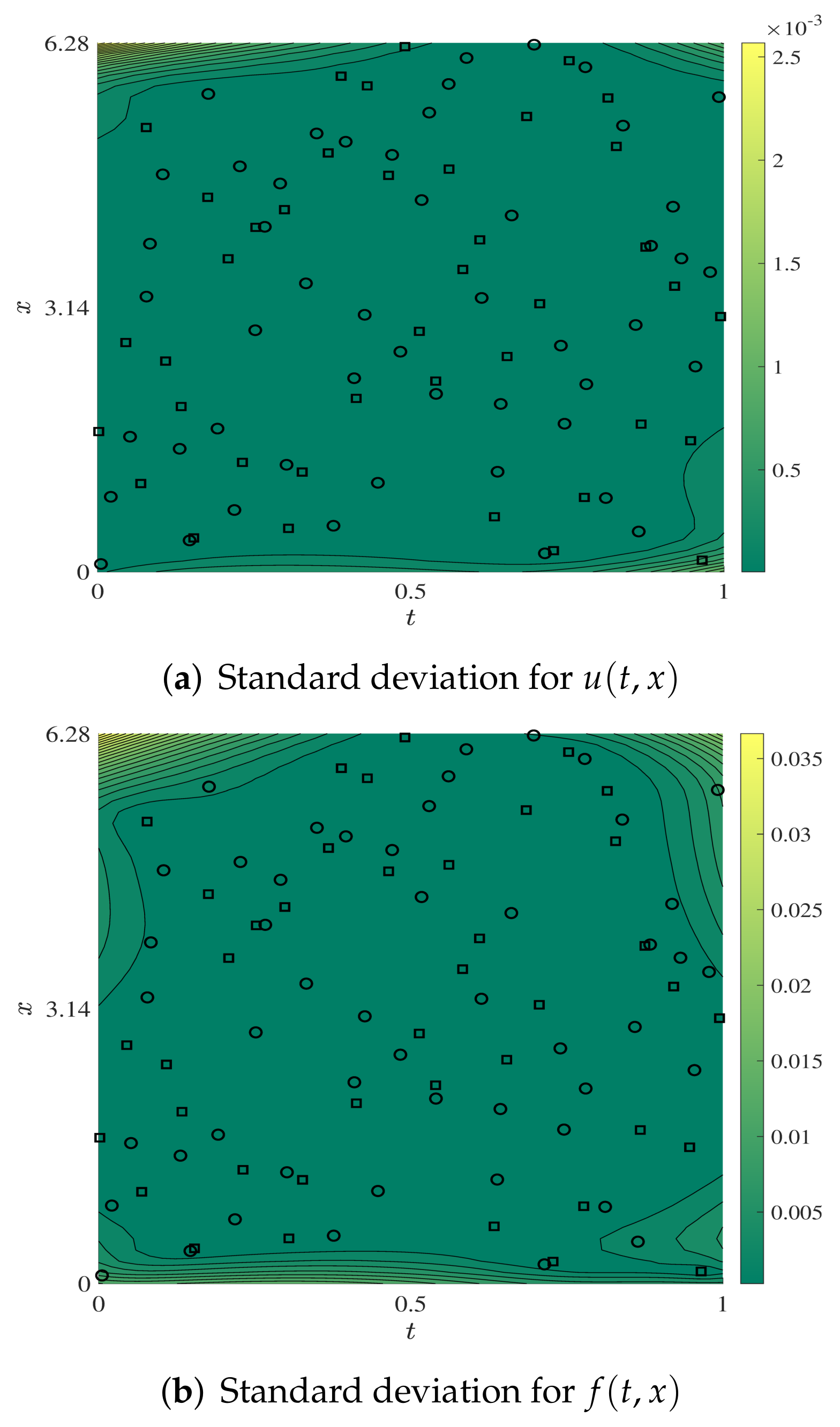
Numerical experiments are performed with the noiseless data of Example 1. We denote that the amount of the training data of u ( t , x ) is N u , and the number of the training data of f ( t , x ) is N f . Take N u = 50 and N f = 40 in this subsection. Fix ( α , β ) to be (1,1), and the estimated value ( α ^ , β ^ ) is (1.014005, 1.014634). Figure 1 shows the distribution of the training data of u ( t , x ) and f ( t , x ) . Figure 2 shows the estimation error | u ¯ ( t , x ) u ( t , x ) | and | f ¯ ( t , x ) f ( t , x ) | of u ( t , x ) and f ( t , x ) , respectively. Figure 3 shows the posterior standard deviation of the corresponding prediction solution. It can be seen from Figure 2 and Figure 3 that the posterior standard deviation is positively correlated with the prediction error. The posterior distribution of Gaussian processes can return a satisfactory numerical approximation to u ( t , x ) and f ( t , x ) .
Table 1 shows the estimation values of ( α , β ) and the relative error L 2 for u ( t , x ) and f ( t , x ) , where ( α , β ) is fixed to be (1, 1), (1, 2), (2, 1) and (2, 2), in turn. Furthermore, the experimental results prove that the results of parameter estimation based on Gaussian processes have relatively high accuracy when high-order PDEs are considered.

4.2. Simulation for a Fractional Partial Differential Equation

Example 2.
L ( t , x ) ϕ u ( t , x ) : = α t α u ( t , x ) Q 2 x 2 u ( t , x ) = f ( t , x ) ,
where ( t , x ) ( , 1 ] × [ 0 , 1 ] ϕ = Q and the fractional order α is a given parameter. Assume 0 < α 1 , and the fractional partial derivative in (20) is defined in the Caputo sense as the following,
α t α u ( t , x ) = 1 Γ ( 1 α ) t 1 ( t τ ) α u ( τ , x ) τ d τ ,
The exact solution is u ( t , x ) = e t ( 1 x ) 2 x 2 and the inhomogeneous term is f ( t , x ) = ( 1 x ) 2 x 2 Γ ( 1 α ) t e τ ( t τ ) α d τ 2 Q e t [ 1 + 6 ( 1 + x ) x ] .
Experiments are performed with noiseless data of Example 2. Table 2 shows the estimation values of Q and the relative error L 2 for u ( t , x ) and f ( t , x ) , where ( α , Q ) is fixed to be (0.25, 1), (0.5, 1), (0.75, 1), (0.25, 2), (0.5,2) and (0.75,2), in turn. The experimental results show that the results of parameter estimation based on Gaussian processes have relatively high accuracy when fractional partial differential equations are considered. Furthermore, the posterior distribution of Gaussian processes can return a satisfactory numerical approximation to u ( t , x ) and f ( t , x ) .

4.3. Simulation for a Partial Integro-Differential Equation

Example 3.
L ( t , x ) ϕ u ( t , x ) : = t u ( t , x ) α Δ u ( t , x ) β 0 t Δ u ( τ , x ) d τ = f ,
where ( t , x ) [ 0 , 1 ] × [ 0 , 1 ] , ϕ = ( α , β ) , and Δ u ( t , x ) = 2 u t 2 + 2 u x 2 . The exact solution is u ( t , x ) = ( 1 + t 3 ) ( 2 x 2 ) , and the inhomogeneous term is f ( t , x ) = 1 2 t [ 12 t + β ( 4 12 t + t 3 ) + 6 ( 1 + β ) t x 2 ] + 2 α [ 1 + t 3 + 3 t ( 2 + x 2 ) ] .
Experiments are performed with the noiseless data of Example 3. Table 3 shows the estimation values of ( α , β ) and the relative error L 2 for u ( t , x ) and f ( t , x ) , where ( α , β ) is fixed to be (1, 1), (1, 2), (2, 1) and (2, 2), in turn. The experimental results show that the results of parameter the estimation based on Gaussian processes have relatively high accuracy when partial integro-differential equations are considered. Furthermore, the posterior distribution of Gaussian processes can return a satisfying numerical approximation to u ( t , x ) and f ( t , x ) .
Moreover, we investigate the impact of the amount of training data and the noise level on the accuracy of the estimation, where ( α , β ) is taken as (1, 1). Table 4 shows the estimation values of ( α , β ) and the relative error L 2 for u ( t , x ) and f ( t , x ) , where N u and N f are fixed to be 10, 20, 30, 40 and 50, in turn. The results show that the larger amount of training data, the higher the prediction accuracy in general. Table 5 shows the estimation values and the relative error L 2 where N u = N f = 20 , and the levels of addictive noise from the training data are taken at different values.
According to Table 5, we can conclude that the method can estimate parameters with relatively gratifying accuracy when noise-free data can not be obtained, although the estimation accuracy is sensitive to the noise of u ( t , x ) , which is likely due to the high complexity of the PDEs considered in this paper. Furthermore, we have to admit that this high sensitivity to the noise of the latent solution u greatly limits the scope of application of Gaussian processes. In summary, this problem deserves further research.

4.4. Simulation for a System of Partial Differential Equations

Example 4.
L ( t , x , y ) ϕ , 1 u + L ( t , x , y ) ϕ , 2 v = u t + a u x x + b v x y = f 1 , L ( t , x , y ) ϕ , 3 u + L ( t , x , y ) ϕ , 4 v = u t t + c u y y + v t + d v x y = f 2 ,
where ( t , x , y ) [ 0 , 1 ] 3 , ϕ = ( a , b , c , d ) . u ( t , x , y ) = e t x ( x 1 ) y ( y 1 ) , v ( t , x , y ) = e t sin ( 2 π x ) cos ( 2 π y ) , f 1 ( t , x , y ) = e t [ ( x 2 x + 2 a ) ( y 2 y ) 4 b π 2 cos ( 2 π x ) sin ( 2 π y ) ] and f 2 ( t , x , y ) = e t [ ( x 2 x ) ( y 2 y + 2 c ) + cos ( 2 π y ) sin ( 2 π x ) 4 d π 2 cos ( 2 π x ) sin ( 2 π y ) ] satisfy Equation (23).
Experiments are performed with noiseless data of Example 4. Denote that the amount of training data of u ( t , x , y ) is N u , the amount of training data v ( t , x , y ) is N v , the amount of training data f 1 ( t , x , y ) is N f 1 , and the amount of training data f 2 ( t , x , y ) is N f 2 . Take N u = N v = 100 and N f 1 = N f 2 = 80 in the experiments.
Table 6 shows the estimation values of (a, b, c, d) and the corresponding prediction errors for u, v, f 1 and f 2 , where (a, b, c, d) is fixed to be (1, 1, 1, 1), (1, 1, 2, 2), (2, 2, 1, 1) and (2, 2, 2, 2), in turn. The experimental results show that the results of parameter estimation based on Gaussian processes have high accuracy, and the posterior distribution of Gaussian processes can return a satisfying numerical approximation to u, v, f 1 and f 2 , when the system of linear PDEs is considered.

5. Conclusions

In this paper, we explored the possibility of using Gaussian processes in solving inverse problems of complex linear partial differential equations, which include high-order partial differential equations, partial integro-differential equations, fractional partial differential equations and a system of partial differential equations. The main points of the Gaussian processes method were to encode the distribution information of the data into kernels (covariance functions) of Gaussian process priors, transform unknown parameters of the linear operators into the hyper-parameters of the kernels, train the parameters and hyper-parameters through minimizing the negative log marginal likelihood and infer the solution of the considered equations.
Numerical experiments showed that the data-driven method based on Gaussian processes had high prediction accuracy when estimating the unknown parameters of the PDEs considered, which proved that Gaussian processes have impressive performance in dealing with linear problems. Furthermore, the posterior distribution of Gaussian processes can return a satisfactory numerical approximation to the latent solution and the inhomogeneous term of the PDEs. However, the estimation accuracy of unknown parameters was sensitive to the noise of the latent solution, which still deserves further research. In the future work, we may focus on how to exploit the Gaussian process to solve the inverse problem of nonlinear PDEs and on how to solve the problem of multi-parameter estimation for fractional partial differential equations.

Author Contributions

All the authors contributed equally to this paper. All authors have read and agreed to the published version of the manuscript.

Funding

This work is supported by National Natural Science Foundation of China (No. 71974204).

Institutional Review Board Statement

Not applicable.

Informed Consent Statement

Not applicable.

Data Availability Statement

Not applicable.

Conflicts of Interest

The authors declare no conflict of interest.

References

  1. Rudy, S.H.; Brunton, S.L.; Proctor, J.L.; Kutz, J.N. Data-driven discovery of partial differential equations. Sci. Adv. 2017, 3, e1602614. [Google Scholar] [CrossRef] [PubMed]
  2. Ghahramani, Z. Probabilistic machine learning and artificial intelligence. Nature 2015, 521, 452–459. [Google Scholar] [CrossRef] [PubMed]
  3. Chen, I.Y.; Joshi, S.; Ghassemi, M.; Ranganath, R. Probabilistic machine learning for healthcare. Annu. Rev. Biomed. Data Sci. 2021, 4, 393–415. [Google Scholar] [CrossRef]
  4. Maslyaev, M.; Hvatov, A.; Kalyuzhnaya, A.V. Partial differential equations discovery with EPDE framework: Application for real and synthetic data. J. Comput. Sci. 2021, 53, 101345. [Google Scholar] [CrossRef]
  5. Lorin, E. From structured data to evolution linear partial differential equations. J. Comput. Phys. 2019, 393, 162–185. [Google Scholar] [CrossRef]
  6. Arbabi, H.; Bunder, J.E.; Samaey, G.; Roberts, A.J.; Kevrekidis, I.G. Linking machine learning with multiscale numerics: Data-driven discovery of homogenized equations. JOM 2020, 72, 4444–4457. [Google Scholar] [CrossRef]
  7. Chang, H.; Zhang, D. Machine learning subsurface flow equations from data. Comput. Geosci. 2019, 23, 895–910. [Google Scholar] [CrossRef]
  8. Martina-Perez, S.; Simpson, M.J.; Baker, R.E. Bayesian uncertainty quantification for data-driven equation learning. Proc. R. Soc. A 2021, 477, 20210426. [Google Scholar] [CrossRef]
  9. Dal Santo, N.; Deparis, S.; Pegolotti, L. Data driven approximation of parametrized PDEs by reduced basis and neural networks. J. Comput. Phys. 2020, 416, 109550. [Google Scholar] [CrossRef]
  10. Raissi, M.; Perdikaris, P.; Karniadakis, G.E. Physics-informed neural networks: A deep learning framework for solving forward and inverse problems involving nonlinear partial differential equations. J. Comput. Phys. 2019, 378, 686–707. [Google Scholar] [CrossRef]
  11. Kaipio, J.; Somersalo, E. Statistical and Computational Inverse Problems; Springer Science & Business Media: New York, NY, USA, 2006. [Google Scholar]
  12. Kremsner, S.; Steinicke, A.; Szölgyenyi, M. A deep neural network algorithm for semilinear elliptic PDEs with applications in insurance mathematics. Risks 2020, 8, 136. [Google Scholar] [CrossRef]
  13. Guo, Y.; Cao, X.; Liu, B.; Gao, M. Soling partial differential equations using deep learning and physical constraints. Appl. Sci. 2020, 10, 5917. [Google Scholar] [CrossRef]
  14. Chen, Z.; Liu, Y.; Sun, H. Physics-informed learning of governing equations from scarce data. Nat. Commun. 2021, 12, 6136. [Google Scholar] [CrossRef]
  15. Gelbrecht, M.; Boers, N.; Kurths, J. Neural partial differential equations for chaotic systems. New J. Phys. 2021, 23, 43005. [Google Scholar] [CrossRef]
  16. Cheung, K.C.; See, S. Recent advance in machine learning for partial differential equation. CCF Trans. High Perform. Comput. 2021, 3, 298–310. [Google Scholar] [CrossRef]
  17. Omidi, M.; Arab, B.; Rasanan, A.H.; Rad, J.A.; Par, K. Learning nonlinear dynamics with behavior ordinary/partial/system of the differential equations: Looking through the lens of orthogonal neural networks. Eng. Comput. 2021, 38, 1635–1654. [Google Scholar] [CrossRef]
  18. Lagergren, J.H.; Nardini, J.T.; Lavigne, G.M.; Rutter, E.M.; Flores, K.B. Learning partial differential equations for biological transport models from noisy spatio-temporal data. Proc. R. Soc. A 2020, 476, 20190800. [Google Scholar] [CrossRef]
  19. Koyamada, K.; Long, Y.; Kawamura, T.; Konishi, K. Data-driven derivation of partial differential equations using neural network model. Int. J. Model. Simul. Sci. Comput. 2021, 12, 2140001. [Google Scholar] [CrossRef]
  20. Kalogeris, I.; Papadopoulos, V. Diffusion maps-aided Neural Networks for the solution of parametrized PDEs. Comput. Methods Appl. Mech. Eng. 2021, 376, 113568. [Google Scholar] [CrossRef]
  21. Rifkin, R.; Yeo, G.; Poggio, T. Regularized least-squares classification. Nato Sci. Ser. Sub Ser. III Comput. Syst. Sci. 2003, 190, 131–154. [Google Scholar]
  22. Drucker, H.; Wu, D.; Vapnik, V.N. Support vector machines for spam categorization. IEEE Trans. Neural Netw. 2002, 10, 1048–1054. [Google Scholar] [CrossRef]
  23. Williams, C.K.; Rasmussen, C.E. Gaussian Processes for Machine Learning; MIT Press: Cambridge, MA, USA, 2006. [Google Scholar]
  24. Raissi, M.; Perdikaris, P.; Karniadakis, G.E. Machine learning of linear differential equations using Gaussian processes. J. Comput. Phys. 2017, 348, 683–693. [Google Scholar] [CrossRef]
  25. Yang, S.; Xiong, X.; Nie, Y. Iterated fractional Tikhonov regularization method for solving the spherically symmetric backward time-fractional diffusion equation. Appl. Numer. Math. 2021, 160, 217–241. [Google Scholar] [CrossRef]
  26. Bernardo, J.M.; Smith, A.F. Bayesian Theory; John Wiley & Sons: Hoboken, NJ, USA, 2009. [Google Scholar]
  27. Oates, C.J.; Sullivan, T.J. A modern retrospective on probabilistic numerics. Stat. Comput. 2019, 29, 1335–1351. [Google Scholar] [CrossRef]
  28. Hennig, P.; Osborne, M.A.; Girolami, M. Probabilistic numerics and uncertainty in computations. Proc. R. Soc. A Math. Phys. Eng. Sci. 2015, 471, 20150142. [Google Scholar] [CrossRef]
  29. Conrad, P.R.; Girolami, M.; Särkkä, S.; Stuart, A.; Zygalakis, K. Statistical analysis of differential equations: Introducing probability measures on numerical solutions. Stat. Comput. 2017, 27, 1065–1082. [Google Scholar] [CrossRef]
  30. Hennig, P. Fast probabilistic optimization from noisy gradients. In Proceedings of the International Conference on Machine Learning PMLR, Atlanta, GA, USA, 17–19 June 2013; pp. 62–70. [Google Scholar]
  31. Kersting, H.; Sullivan, T.J.; Hennig, P. Convergence rates of Gaussian ODE filters. Stat. Comput. 2020, 30, 1791–1816. [Google Scholar] [CrossRef]
  32. Raissi, M.; Karniadakis, G.E. Hidden physics models: Machine learning of nonlinear partial differential equations. J. Comput. Phys. 2018, 357, 125–141. [Google Scholar] [CrossRef]
  33. Raissi, M.; Perdikaris, P.; Karniadakis, G.E. Inferring solutions of differential equations using noisy multi-fidelity data. J. Comput. Phys. 2017, 335, 736–746. [Google Scholar] [CrossRef]
  34. Raissi, M.; Perdikaris, P.; Karniadakis, G.E. Numerical Gaussian processes for time-dependent and nonlinear partial differential equations. SIAM J. Sci. Comput. 2018, 40, A172–A198. [Google Scholar] [CrossRef]
  35. Scholkopf, B.; Smola, A.J.; Bach, F. Learning with Kernels: Support Vector Machines, Regularization, Optimization, and Beyond; MIT Press: Cambridge, MA, USA, 2002. [Google Scholar]
  36. Tipping, M.E. Sparse Bayesian learning and the relevance vector machine. J. Mach. Learn. Res. 2001, 1, 211–244. [Google Scholar]
  37. Konig, H. Eigenvalue Distribution of Compact Operators; Birkhäuser: Basel, Switzerland, 2013. [Google Scholar]
  38. Berlinet, A.; Thomas-Agnan, C. Reproducing Kernel Hilbert Spaces in Probability and Statistics; Springer Science & Business Media: Berlin/Heidelberg, Germany, 2011. [Google Scholar]
  39. Zhu, C.; Byrd, R.H.; Lu, P.; Nocedal, J. Algorithm 778: L-BFGS-B: Fortran subroutines for large-scale bound-constrained optimization. ACM Trans. Math. Softw. (TOMS) 1997, 23, 550–560. [Google Scholar] [CrossRef]
  40. Mirjalili, S.; Lewis, A. The whale optimization algorithm. Adv. Eng. Softw. 2016, 95, 51–67. [Google Scholar] [CrossRef]
  41. Dorigo, M.; Stützle, T. Ant colony optimization: Overview and recent advances. In Handbook of Metaheuristics; Springer: Cham, Switzerland, 2019. [Google Scholar]
  42. Raissi, M.; Babaee, H.; Karniadakis, G.E. Parametric Gaussian process regression for big data. Comput. Mech. 2019, 64, 409–416. [Google Scholar] [CrossRef]
  43. Snelson, E.; Ghahramani, Z. Sparse Gaussian processes using pseudo-inputs. In Advances in Neural Information Processing Systems 18 (NIPS 2005); MIT Press: Cambridge, MA, USA, 2005. [Google Scholar]
  44. Liu, H.; Ong, Y.S.; Shen, X.; Cai, J. When Gaussian process meets big data: A review of scalable GPs. IEEE Trans. Neural Netw. Learn. Syst. 2020, 31, 4405–4423. [Google Scholar] [CrossRef]
  45. Milici, C.; Draganescu, G.; Machado, J.T. Introduction to Fractional Differential Equations; Springer: Cham, Switzerland, 2018. [Google Scholar]
  46. Podlubny, I. Fractional Differential Equations; Academic Press: San Diego, CA, USA, 1998. [Google Scholar]
  47. Povstenko, Y. Linear Fractional Diffusion-Wave Equation for Scientists and Engineers; Birkhäuser: New York, NY, USA, 2015. [Google Scholar]
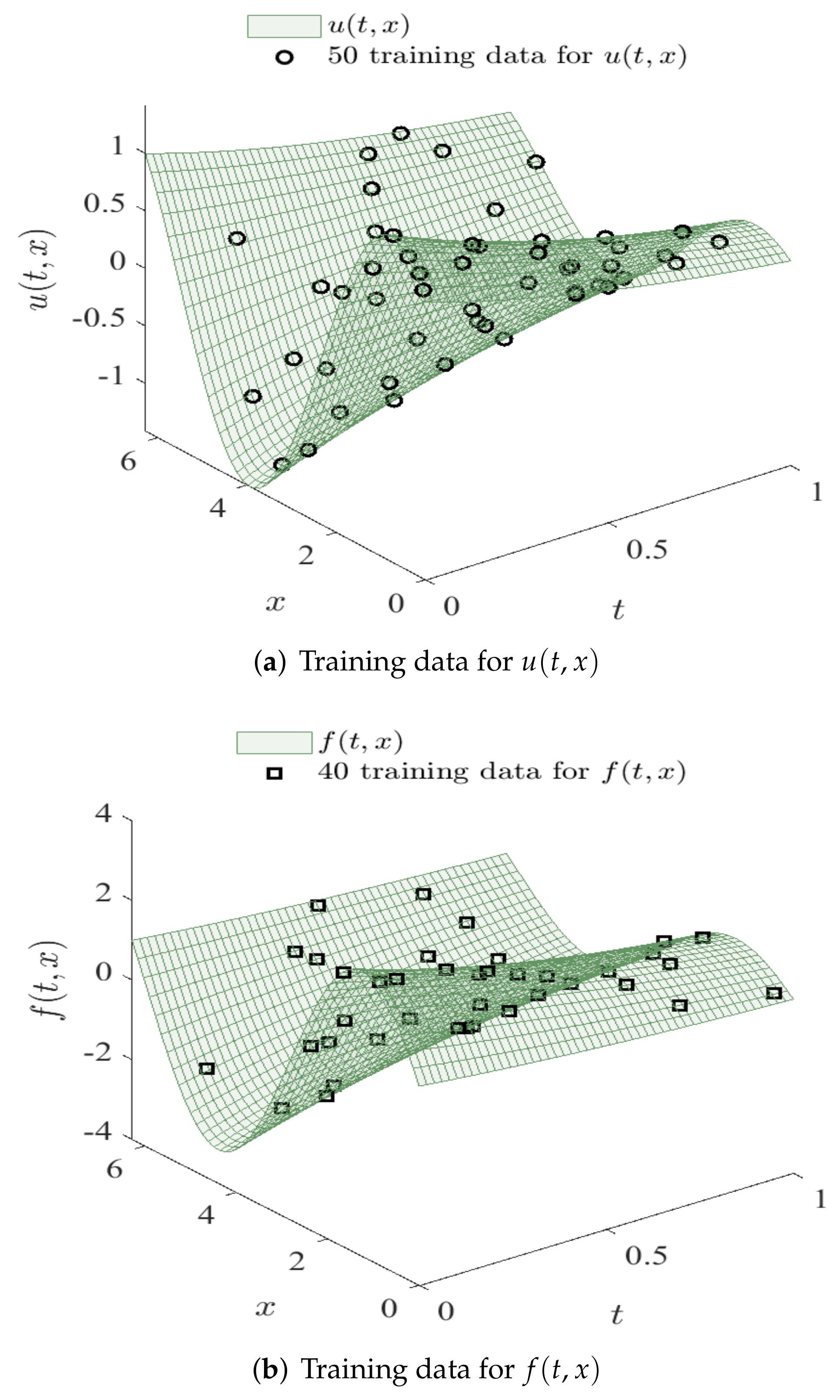
Figure 1. High-order partial differential equation: training data for u ( t , x ) and f ( t , x ) .
Fractalfract 06 00433 g001
Figure 2. High-order partial differential equation: prediction error for u ( t , x ) and f ( t , x ) .
Fractalfract 06 00433 g002
Figure 3. High-order partial differential equation: Standard deviation for u ( t , x ) and f ( t , x ) .
Fractalfract 06 00433 g003
Table 1. High-order partial differential equation: estimated values of ( α , β ) and the relative error L 2 for u ( t , x ) and f ( t , x ) , where N u = 50 , N f = 40 , and ( α , β ) is fixed to be (1, 1), (1, 2), (2, 1) and (2, 2) in turn.
α ^ 1.0140051.0217242.0068562.008363
β ^ 1.0146342.0329891.0064082.020304
L 2 for u3.201 × 10 4 5.615 × 10 4 1.869 × 10 4 3.319 × 10 4
L 2 for f2.665 × 10 3 1.825 × 10 3 3.037 × 10 3 2.823 × 10 3
Table 2. Fractional partial differential equation: estimated values of Q and the relative error L 2 for u ( t , x ) and f ( t , x ) where N u = 15 , N f = 12 , ( α , Q ) is fixed to be (0.25, 1), (0.5, 1), (0.75, 1), (0.25, 2), (0.5, 2) and (0.75, 2), in turn.
( α , Q ) ( 0.25 , 1 ) ( 0.5 , 1 ) ( 0.75 , 1 ) ( 0.25 , 2 ) ( 0.5 , 2 ) ( 0.75 , 2 )
Q ^ 1.0002621.0001150.9994362.0008101.9998361.995571
L 2 for u1.147 × 10 2 1.075 × 10 2 8.409 × 10 3 8.935 × 10 3 8.555 × 10 3 7.244 × 10 3
L 2 for f1.562 × 10 1 1.552 × 10 1 1.488 × 10 1 1.462 × 10 1 1.474 × 10 1 1.524 × 10 1
Table 3. Partial integro-differential equation: estimated values of ( α , β ) and the relative error L 2 for u ( t , x ) and f ( t , x ) , where N u = 20 , N f = 20 , ( α , β ) is fixed to be (1, 1), (1, 2), (2, 1) and (2, 2), in turn.
( α , β ) ( 1 , 1 ) ( 1 , 2 ) ( 2 , 1 ) ( 2 , 2 )
α ^ 1.0001030.9992822.0007692.000163
β ^ 0.9994682.0016180.9969791.998910
L 2 for u3.077 × 10 5 6.223 × 10 5 4.726 × 10 5 3.202 × 10 5
L 2 for f6.331 × 10 3 4.784 × 10 3 5.294 × 10 3 3.857 × 10 3
Table 4. Numerical results for Example 3. Impact of the amount of training data: estimated values of ( α , β ) and the relative error L 2 for u ( t , x ) and f ( t , x ) , where ( α , β ) is fixed to be (1,1) and noise-free data is used.
N u = N f 1020304050
α ^ 0.8872391.0001030.9997631.0000570.999051
β ^ 1.3439890.9994681.0011560.9996101.005044
L 2 for u1.979 × 10 2 3.077 × 10 5 6.761 × 10 6 2.510 × 10 6 2.752 × 10 5
L 2 for f1.759 × 10 2 6.331 × 10 3 6.737 × 10 4 4.779 × 10 4 9.552 × 10 5
Table 5. Numerical results for Example 3. Impact of the levels of addictive noise: estimated values of ( α , β ) and the relative error L 2 for u ( t , x ) and f ( t , x ) where N u = N f = 20 , ( α , β ) is fixed to be (1,1).
( σ u 2 , σ f 2 ) ( 0 , 0 ) ( 0 , 0 . 5 2 ) ( 0 , 1 . 0 2 ) ( 0 . 005 2 , 0 ) ( 0 . 005 2 , 0 . 5 2 ) ( 0 . 005 2 , 1 . 0 2 )
α ^ 1.0001030.9831240.9770750.9746450.9416510.926553
β ^ 0.9994681.1255531.2434691.4508931.5117681.582164
L 2 for u3.077 × 10 5 1.467 × 10 3 1.684 × 10 3 4.594 × 10 3 4.274 × 10 3 5.241 × 10 3
L 2 for f6.331 × 10 3 1.134 × 10 1 1.483 × 10 1 3.814 × 10 3 1.800 × 10 1 2.734 × 10 1
Table 6. A system of partial differential equations: estimated values of (a, b, c, d) and the relative error L 2 for u, v, f 1 and f 2 , where N u 1 = N u 2 = 100 , N f 1 = N f 2 = 80 , and (a, b, c, d) is fixed to be (1, 1, 1, 1), (1, 1, 2, 2), (2, 2, 1, 1) and (2, 2, 2, 2), in turn.
(a, b, c, d) ( 1 , 1 , 1 , 1 ) ( 1 , 1 , 2 , 2 ) ( 2 , 2 , 1 , 1 ) ( 2 , 2 , 2 , 2 )
a ^ 1.0008031.0008282.0010612.000685
b ^ 1.0001201.0001122.0002562.000255
c ^ 0.9996392.0009540.9989052.000404
d ^ 0.9999271.9998790.9999351.999898
L 2 for u1.363 × 10 2 1.409 × 10 2 1.215 × 10 2 1.230 × 10 2
L 2 for v4.805 × 10 3 4.601 × 10 3 4.754 × 10 3 4.395 × 10 3
L 2 for f 1 1.383 × 10 2 1.368 × 10 2 1.354 × 10 2 1.335 × 10 2
L 2 for f 2 1.396 × 10 2 1.374 × 10 2 1.366 × 10 2 1.339 × 10 2
Publisher’s Note: MDPI stays neutral with regard to jurisdictional claims in published maps and institutional affiliations.