Local Stabilization of Delayed Fractional-Order Neural Networks Subject to Actuator Saturation

Abstract

This paper investigates the local stabilization problem of delayed fractional-order neural networks (FNNs) under the influence of actuator saturation. First, the sector condition and dead-zone nonlinear function are specially introduced to characterize the features of the saturation phenomenon. Then, based on the fractional-order Lyapunov method and the estimation technique of the Mittag–Leffler function, an LMIs-based criterion is derived to guarantee the local stability of closed-loop delayed FNNs subject to actuator saturation. Furthermore, two corresponding convex optimization schemes are proposed to minimize the actuator costs and expand the region of admissible initial values, respectively. At last, two simulation examples are developed to demonstrate the feasibility and effectiveness of the derived results.

1. Introduction

With the rapid development of fractional derivative theory, many fractional-order models have been newly built by using fractional-order differential equations [1,2,3,4,5,6]. In contrast with the integer-order cases, the heredity and memory of various processes are consistent with fractional-order models. For example, the recent works have displayed that the dynamical behaviors of pyramidal neurons can be described accurately based on fractional-order differentiation [6]. Accordingly, the application of the fractional derivative has gained increasing attention in recent years. It should be mentioned that the corresponding experiments have demonstrated that the practical capacitors, as for electronic circuits, are with the characteristics of fractional order. In combination with Kirchhoff’s current law, one can obtain the voltage current relation, i.e., $i\left(t\right)=C\frac{d^{\alpha }V\left(t\right)}{d{t}^{\alpha }}\triangleq C_0{D}_t^{\alpha }V\left(t\right)$ [5,7], and thus, the so-called FNNs are established. Thereinto, $\alpha$ denotes the posses of capacitors. Compared with the traditional integer-order neural networks [8], it is more useful and significant to imitate the behavior of brain neurons. At the same time, time delays are unavoidable in the transmission channels, which will cause oscillation or chaos in practical applications [9]. For instance, when choose the time delays as bifurcation parameters, the Hopf bifurcation and stability issues have been addressed for complex-valued FNNs by using the Laplace transforms and fractional-order differential equations theory [10]. Therefore, it is very important to research the dynamical analysis of delayed FNNs and a lot of excellent results such as stability [11,12,13,14], global stabilization [15,16,17], synchronization [18,19], and dissipativity [20,21] have been well reported.

Notice that the published results are obtained in a perfect communication environment. That is, the control input is unlimited. For instance, the $\mu$-type synchronization control problem has been discussed for a type of FNNs by designing a linear feedback controller [22]. The global stabilization problem has been addressed for FNN based on the comparison principle and positive-system-dependent method [23]. In addition, the adaptive synchronization behavior has been solved for FNNs by designing the adaptive quantized control law [18]. Nevertheless, the control input is usually restricted owing to the limitation of amplification capacity and switching frequency of the applied amplification circuits [24,25,26,27]. As such, it is important to consider the stability issue for delayed FNNs in the presence of actuator saturation. At present, two useful approaches, i.e., polytopic representation approach [24,25] and sector model approach [26,27], have been proposed to deal with the actuator saturation problem. For example, the local stabilization issue has been solved for integer-order memristive neural networks by employing discrete-time and continuous-time Lyapunov theories [26]. Furthermore, an adaptive control method has been studied for a type of robotic manipulators with input saturation in view of the Lyapunov–Krasovskii functional method [28]. Although the above-mentioned analysis techniques are well used to guarantee the stability of integer-order systems, these methods cannot be applied to fractional-order systems, since they are characterized in the form of fractional-order differential equations [29,30]. Accordingly, it is challenging to investigate the stabilization issue of delayed FNNs with actuator saturation. This is the first motivation.

As is well known, it is impossible to achieve the global stabilization for delayed FNNs under the influence of actuator saturation [31,32]. As such, a key issue is how to estimate the safety working area, i.e., admissible initial values, as large as possible. It means that the local stability can be achieved if the selected initial values belong to the safety working area. To this end, the corresponding convex optimization methods have been used to solve this problem. Notice that the premise of using these optimization conditions is that the stability conditions are given by LMIs. Nevertheless, most of the above results, as for fractional-order systems, are algebraic conditions rather than LMIs-based conditions. The algebraic conditions of exponential stability and synchronization, via impulsive control, have been obtained for fractional-order systems [11]. The algebraic conditions of finite-time stability, by using Gronwall’s inequality method, have been developed for delayed fractional-order systems with nonlinear perturbation [14]. Furthermore, the algebraic conditions of stabilization have been established for delayed FNNs with bidirectional associative memory by employing Barbalat lemma and some fractional-order inequalities [17]. Namely, these used analysis techniques cannot be applied to establish convex optimization schemes. To this end, in recent years, some LMIs-based stability techniques have been proposed for fractional-order systems. For example, the LMIs-based conditions of global stability and synchronization have been proposed for FNNs based on the fractional-order Lyapunov method [19]. In addition, the LMIs-based conditions of local Mittag–Leffler stabilization have been developed for FNNs subject to actuator saturation, and the corresponding LMIs-based optimization schemes have been derived [33]. However, the applied analysis methods are no longer applicable because the time delay is considered in this paper. Accordingly, how to derive the corresponding convex optimization schemes is an urgent question in the presence of the time delay and actuator saturation. Before this, three core problems need to be solved: (1) how to design feedback controller gain against actuator saturation; (2) how to obtain the LMIs-based stability conditions under the influence of time delay; and (3) based on (2), how to design convex optimization schemes to minimize the actuator costs and enlarge the region of admissible initial values. These provide the second motivation.

In order to answer the previous discussions and motivations, the local stabilization of delayed FNNs is investigated suffer from actuator saturation. The main works are included as follows:

(1)

According to the feature of actuator saturation, a dead-zone nonlinear function is used to design the feedback control gain matrix from the saturation function. Then, a novel closed-loop model is derived, which can contribute to the stability analysis.

(2)

In view of the fractional-order Lyapunov theory and the estimation technique of Mittag–Leffler function, an LMIs-based stability condition is derived for the closed-loop systems. On this basis, two optimization schemes, by applying convex optimization techniques, are respectively proposed to enlarge the region of admissible initial values and minimize the actuator costs.

In this paper,

Table 1. Notations and Descriptions.

Notation	Description
diag$(\cdots )$	a block diagonal matrix
LMIs	linear matrix inequalities
$E>0$	E is a positive
(or $E\ge 0)$	definite (or semi-definite) matrix
$E^T\left(\mathrm{or}{E}^{-1}\right)$	transpose (or inverse) of matrix E
∗	the symmetric element
$E_{\left(i\right)}$	the i-th row of matrix E
${\lambda }_{max}\left(E\right)$	the maximum eigenvalue of matrix E
0	zero (or identity) matrices
$\left(\mathrm{or}I\right)$	of appropriate dimensions

shows some useful notations.

2. Preliminaries and Problem Formulation

Consider the following n-dimensional delayed FNNs with input saturation as follows:

$${}_0{D}_t^{\alpha }{z}_{}\left(t\right)=-D_{}^{}{z}_{}\left(t\right)+M{f}_{}\left(z_{}\left(t\right)\right)+W{g}_{}\left(z_{}(t-\varrho )\right)+u\left(t\right),$$

(1)

where $z\left(t\right)={[z_1\left(t\right),z_2\left(t\right),\cdots ,z_n\left(t\right)]}^T$ denotes the state vector. $D=\mathrm{diag}(d_1,d_2,\cdots ,d_n)>0$, $M={\left(m_{ij}\right)}_{n\times n}$ and $W={\left(m_{ij}\right)}_{n\times n}$ are connection weight matrices. $g\left(z\right(t-\varrho \left)\right)$, $f\left(z\right(t)$ are the activation functions. The initial condition is denoted as $z\left(s\right)=z\left(0\right),z\in [-\varrho ,0]$. $\varrho$ is the time delay. $u\left(t\right)=\mathrm{sat}\left(Kz\right(t\left)\right)$ denotes the saturation controller and K is the feedback control gain. $\mathrm{sat}\left(Kz\right(t\left)\right)$ represents the saturated function defined by

$$\mathrm{sat}\left(K_{\left(i\right)}z\left(t\right)\right)=\mathrm{sgn}\left(K_{\left(i\right)}z\left(t\right)\right)min\left\{|K_{\left(i\right)}z\left(t\right)|,u_{\left(i\right)}\right\},i=1,\dots ,n,$$

with the saturation levels $u_i>0$.

A dead-zone nonlinear function $\psi \left(Kz\right(t\left)\right)$ [24], aiming at handling the saturation term, is defined as

$$\psi \left(Kz\right(t\left)\right)=Kz\left(t\right)-\mathrm{sat}\left(Kz\right(t\left)\right).$$

Then, one rewrites system (1) as follows:

$$\begin{array}{cc}\hfill {}_0{D}_t^{\alpha }z\left(t\right)=& -Dz\left(t\right)+Mf\left(z\left(t\right)\right)+W{g}_{}\left(z_{}(t-\varrho )\right)+Kz\left(t\right)-\psi \left(Kz\left(t\right)\right).\hfill \end{array}$$

(2)

Assumption 1.

The $f_j(·)$ and $g_j(·)$ are assumed to be monotonically non-decreasing and Lipschitz-continuous; namely, there exist Lipschitz constants $F_j$ and $G_j$ such that

$$0\le \frac{f_j\left(\gamma \right)-f_j\left(v\right)}{\gamma -v}\le F_j,0\le \frac{g_j\left(\gamma \right)-g_j\left(v\right)}{\gamma -v}\le G_j,$$

for $j=1,2,\cdots ,n$, $\gamma ,v\in \mathbb{R}$, $\gamma \ne v$.

Define a polyhedral set

$$\mathsf{{\rm Y}}=\left\{z\in {\mathbb{R}}^n\left|\right|(K_{\left(i\right)}-Q_{\left(i\right)})z|\le u_{\left(i\right)}\right\},$$

where $i=1,\dots ,n$, $Q\in {\mathbb{R}}^{n\times n}$. Then, for any diagonal matrix $N>0$, if $z\left(t\right)\in \mathsf{{\rm Y}}$, the following sector condition [24] holds

$$-{\mathsf{\Psi }}^T\left(Kz\left(t\right)\right)N[\mathsf{\Psi }\left(Kz\left(t\right)\right)-Qz\left(t\right)]\ge 0.$$

(3)

Definition 1

([1]). The Caputo fractional derivative ${}_0{D}_t^{\alpha }x\left(t\right)$, Mittag–Leffler function are defined as

$${}_0{D}_t^{\alpha }x\left(t\right)=\frac{1}{\mathsf{\Gamma }(1-\alpha )}{\int }_0^t{(t-\varrho )}^{-\alpha }{x}^{\prime }\left(\varrho \right)d\varrho ,$$

$$E_{\alpha ,\beta }\left(y\right)={\mathsf{\Sigma }}_{k=0}^{k=\infty }\frac{y^k}{\mathsf{\Gamma }(k\alpha +\beta )},$$

where $t\ge 0$, $y\in \mathbb{C}$, $0<\alpha <1$, $\beta >0$, and $\mathsf{\Gamma }\left(\alpha \right)={\int }_0^{+\infty }{e}^{-t}{t}^{\alpha -1}dt$. 0 denotes the initial time. $x\left(t\right)$ is a function. When $\beta =1$, it has $E_{\alpha ,\beta }\left(y\right)=E_{\alpha }\left(y\right)$.

Definition 2.

The closed-loop system (1) is said to be locally stable if for any trivial solutions $z\left(t\right)$ with initial values $z\left(s\right)\in \eta \left(P\right)$, $s\in [-\varrho ,0]$, belonging to the set $\eta \left(P\right)=\{z\in {\mathbb{R}}^n:z^{T}Pz\le 1\}$, such as

$$\underset{t\to +\infty }{lim}{\left|\right|z\left(t\right)\left|\right|}_2=0,$$

where $P>0$.

Lemma 1

([34]). Consider a matrix $P>0$, one has

$${\frac{1}{2}}_0{D}_t^{\alpha }{z}^T\left(t\right)Pz\left(t\right)\le z^T\left(t\right)P_0{D}_t^{\alpha }z\left(t\right),\forall \alpha \in (0,1],$$

where $z\left(t\right)\in R^n$ denotes a continuous function.

Lemma 2

([29]). For $0<\alpha <1$, $-\infty <t<+\infty$, one has

$$E_{\alpha }\left(t\right)>0,\frac{d}{dt}{E}_{\alpha ,\alpha }\left(t\right)>0,E_{\alpha ,\alpha }\left(t\right)>0.$$

Lemma 3

([24]). For matrix $R>0$, a non-singular matrix J, and $\tilde{R}=J^{T}RJ$, if

$$\left[\begin{array}{cc}{R}_0& I\\ I& J+J^T-\tilde{R}\end{array}\right]>0,$$

then $R<R_0$ holds.

3. Main Results

Theorem 1.

For given parameters $\delta >0$, $ϵ>0$, and $n\times n$-matrices Q, K, if there exists an $n\times n$-matrix $P>0$, and diagonal matrices $N>0$, $U_1>0,U_2>0$, such that the following LMIs (4)–(6) are satisfied

$$\Theta =\left[\begin{array}{ccccc}{\Theta }_{11}& 0& PM+F{U}_1& PW& -P+Q^{T}N\\ \ast & -ϵP& 0& G{U}_2& 0\\ \ast & \ast & -2U_1& 0& 0\\ \ast & \ast & \ast & -2U_2& 0\\ \ast & \ast & \ast & \ast & -2N\end{array}\right]<0,$$

(4)

$$\left[\begin{array}{cc}P& {(K_{\left(i\right)}-Q_{\left(i\right)})}^T\\ \ast & u_{\left(i\right)}^2\end{array}\right]\ge 0,$$

(5)

$$\delta -ϵ>0,$$

(6)

where ${\Theta }_{11}=-PD-DP+PK+K^{T}P+\delta P$, $G=diag(G_1,G_2,\dots$, $G_n)$, $F=diag(F_1,F_2,\dots ,F_n)$. Then, for any initial values $z\left(s\right)\in \eta \left(P\right)$, $s\in [-\varrho ,0]$, $\eta \left(P\right)=\{z\in {\mathbb{R}}^n:z^{T}Pz\le 1\}$, the closed-loop system (2) is locally asymptotically stable.

Proof. 

Choose the auxiliary Lyapunov function as follows:

$$V\left(t\right)=z^T\left(t\right)Pz\left(t\right).$$

Using Lemma 1, one has

$$\begin{array}{cc}\hfill {}_0{D}_t^{\alpha }V\left(t\right)& \le 2z^T\left(t\right)P_0{D}_t^{\alpha }z\left(t\right).\hfill \end{array}$$

(7)

Based on the characteristics of $g\left(z\right(t-\varrho \left)\right)$, $f\left(z\right(t\left)\right)$, for diagonal matrices $U_1>0,U_2>0$, one can obtain

$$\begin{array}{cc}\hfill 0& \le 2\left[\begin{array}{cc}{z}^T\left(t\right)& f^T\left(z\left(t\right)\right)\end{array}\right]\left[\begin{array}{cc}0& \frac{F{U}_1}{2}\\ \ast & -U_1\end{array}\right]\left[\begin{array}{c}z\left(t\right)\\ f\left(z\right(t\left)\right)\end{array}\right].\hfill \end{array}$$

(8)

$$\begin{array}{cc}\hfill 0& \le 2\left[\begin{array}{cc}{z}^T(t-\varrho )& g^T\left(z(t-\varrho )\right)\end{array}\right]\left[\begin{array}{cc}0& \frac{G{U}_2}{2}\\ \ast & -U_2\end{array}\right]\left[\begin{array}{c}z(t-\varrho )\\ g\left(z\right(t-\varrho \left)\right)\end{array}\right].\hfill \end{array}$$

(9)

Based on (2), (3), and (7)–(9), one has

$$\begin{array}{cc}\hfill {}_0{D}_t^{\alpha }V\left(t\right)& \le 2z^T\left(t\right)P[-D_{}^{}{z}_{}\left(t\right)+M{f}_{}\left(z_{}\left(t\right)\right)+W{g}_{}\left(z_{}(t-\varrho )\right)+Kz\left(t\right)-\psi \left(Kz\left(t\right)\right)]\hfill \\ \hfill & -2{\psi }^T\left(Kz\left(t\right)\right)N\psi \left(Kz\left(t\right)\right)+2{\psi }^T\left(Kz\left(t\right)\right)NQz\left(t\right)+2f^T\left(z\left(t\right)\right)U_{1}Fz\left(t\right)\hfill \\ \hfill & -2f^T\left(z\left(t\right)\right)U_{1}f\left(z\left(t\right)\right)+2g^T\left(z(t-\varrho )\right)U_{2}Gz(t-\varrho )-2g^T\left(z(t-\varrho )\right)U_{2}g\left(z(t-\varrho )\right)\hfill \\ \hfill & +\delta z^T\left(t\right)Pz\left(t\right)-ϵz^T(t-\varrho )Pz(t-\varrho )-\delta V\left(t\right)+ϵV(t-\varrho )\hfill \\ \hfill & ={\rho }^T\left(t\right)\Theta \rho \left(t\right)-\delta V\left(t\right)+ϵV(t-\varrho ),\hfill \end{array}$$

where $\rho \left(t\right)={[z^T\left(t\right),z^T(t-\varrho ),f^T\left(z\left(t\right)\right),g^T\left(z(t-\varrho )\right),{\psi }^T\left(Kz\left(t\right)\right)]}^T$.

By using (4), one has

$$\begin{array}{cc}\hfill {}_0{D}_t^{\alpha }V\left(t\right)& \le -\delta V\left(t\right)+ϵV(t-\varrho )\hfill \\ \hfill & \le -\delta V\left(t\right)+ϵ\underset{t-\varrho \le \xi \le t}{sup}V\left(\xi \right).\hfill \end{array}$$

Thus, for a non-negative function $\kappa \left(t\right)$, it yields

$$\begin{array}{c}\hfill {}_0{D}_t^{\alpha }V\left(t\right)+\kappa \left(t\right)=-\delta V\left(t\right)+ϵ\underset{t-\varrho \le \xi \le t}{sup}V\left(\xi \right).\end{array}$$

(10)

By solving (10), one can obtain

$$\begin{array}{c}\hfill V\left(t\right)={\int }_0^t\frac{E_{\alpha ,\alpha }(-\delta {(t-s)}^{\alpha })[ϵ{sup}_{s-\varrho \le \xi \le s}V\left(\xi \right)-\kappa \left(s\right)]}{{(t-s)}^{1-\alpha }}ds+V\left(0\right)E_{\alpha }(-\delta t^{\alpha }).\end{array}$$

(11)

Owing to $\kappa \left(t\right)\ge 0$, from Lemma 2, it yields

$$V\left(t\right)\le ϵ\underset{-\varrho \le \xi \le t}{sup}V\left(\xi \right){\int }_0^t\frac{E_{\alpha ,\alpha }(-\delta {(t-s)}^{\alpha })}{{(t-s)}^{1-\alpha }}ds+V\left(0\right)E_{\alpha }(-\delta t^{\alpha }).$$

Notice that $p\left(t\right)\triangleq {\int }_0^t\frac{E_{\alpha ,\alpha }(-\delta {(t-s)}^{\alpha })}{{(t-s)}^{1-\alpha }}ds=t^{\alpha }{E}_{\alpha ,1+\alpha }(-\delta t^{\alpha })$. Thus, by using the asymptotic expansion [1], one can obtain $0<p\left(t\right)<\frac{1}{\delta }$, $0<E_{\alpha }(-\delta t^{\alpha })<1$. Then, one has

$$V\left(t\right)\le V\left(0\right)+\frac{ϵ}{\delta }\underset{-\varrho \le \xi \le t}{sup}V\left(\xi \right).$$

Combined with (6) and the Lemma 2.1 in [30], it can be derived that

$$V\left(t\right)\le \frac{\delta }{\delta -ϵ}V\left(0\right)+M_0,t>0,$$

where $M_0={sup}_{-\varrho \le \xi \le 0}V\left(\xi \right)$. Hence, $V\left(t\right)$ is bounded in $t\in [0,+\infty )$, that is, $V\left(t\right)\le \frac{\delta }{\delta -ϵ}V\left(0\right)+M_0=Y_0$. Obviously, the supremum $R\left(t\right)={sup}_{\xi \in [t,+\infty )}V\left(\xi \right)$ exists and decreases monotonically for any $t\in [0,+\infty )$. Aiming at deriving the upper bound of $V\left(t\right)$, $t\to +\infty$, from (11), it can be obtained that

$$\begin{array}{c}\hfill V\left(t\right)\le ϵ{\int }_0^t\frac{E_{\alpha ,\alpha }(-\delta {(t-s)}^{\alpha }){sup}_{s-\varrho \le \xi \le s}V\left(\xi \right)}{{(t-s)}^{1-\alpha }}ds+V\left(0\right)E_{\alpha }(-\delta t^{\alpha }).\end{array}$$

(12)

Set ${lim}_{t\to +\infty }R\left(t\right)=R$. Then, there exists $t_1>0$ such that ${sup}_{\xi \in [t_1,+\infty )}V\left(\xi \right)<R+{\iota }_1$, $t>t_1$. It should be mentioned that ${lim}_{t\to +\infty }(t-\varrho )=+\infty$; then, there also exists $t_2\ge t_1$ such that $t-\varrho \ge t_1$ for any $t\ge t_2>0$. Thus, one has

$$\underset{\xi \in [t-\varrho ,t]}{sup}V\left(\xi \right)\le \underset{\xi \in [t_1,t]}{sup}V\left(\xi \right)\le R+{\iota }_1,t\ge t_2.$$

Meanwhile, for any given ${\iota }_2$, it has

$$\underset{t\to +\infty }{lim}\underset{s\in [t,+\infty )}{sup}{\int }_0^{t_2}\frac{E_{\alpha ,\alpha }(-\delta {(s-r)}^{\alpha })}{{(s-r)}^{1-\alpha }}dr\le \underset{t\to +\infty }{lim}\underset{s\in [t,+\infty )}{sup}\frac{t_2}{{(s-t_2)}^{1-\alpha }}<{\iota }_2.$$

From the above analysis, it yields

$$\begin{array}{cc}\hfill & \underset{t\to +\infty }{lim}\underset{s\in [t,+\infty )}{sup}{\int }_0^s\frac{E_{\alpha ,\alpha }(-\delta {(s-r)}^{\alpha }){sup}_{r-\varrho \le \xi \le r}V\left(\xi \right)}{{(s-r)}^{1-\alpha }}dr\hfill \\ \hfill & =\underset{t\to +\infty }{lim}\underset{s\in [t,+\infty )}{sup}{\int }_0^{t_3}\frac{E_{\alpha ,\alpha }(-\delta {(s-r)}^{\alpha }){sup}_{r-\varrho \le \xi \le r}V\left(\xi \right)}{{(s-r)}^{1-\alpha }}dr\hfill \\ \hfill & +\underset{t\to +\infty }{lim}\underset{s\in [t,+\infty )}{sup}{\int }_{t_3}^s\frac{E_{\alpha ,\alpha }(-\delta {(s-r)}^{\alpha }){sup}_{r-\varrho \le \xi \le r}V\left(\xi \right)}{{(s-r)}^{1-\alpha }}dr\hfill \\ \hfill & \le Y_0\underset{t\to +\infty }{lim}\underset{s\in [t,+\infty )}{sup}{\int }_0^{t_3}\frac{E_{\alpha ,\alpha }(-\delta {(s-r)}^{\alpha })}{{(s-r)}^{1-\alpha }}dr\hfill \\ \hfill & +(R+{\iota }_1)\underset{t\to +\infty }{lim}\underset{s\in [t,+\infty )}{sup}{\int }_{t_3}^s\frac{E_{\alpha ,\alpha }(-\delta {(s-r)}^{\alpha })}{{(s-r)}^{1-\alpha }}dr\hfill \\ \hfill & \le Y_0{\iota }_2+\frac{R+{\iota }_1}{\delta }.\hfill \end{array}$$

On the other hand, ${lim}_{t\to +\infty }{E}_{\alpha }(-\delta t^{\alpha })=0$. Accordingly, there exists $t_3>0$ for any given ${\iota }_3>0$ such that

$$\begin{array}{c}\hfill V\left(0\right)E_{\alpha }(-\delta t^{\alpha })\le {\iota }_3,t\ge t_3.\end{array}$$

Combined with inequality (12), one has

$$R=\underset{t\to +\infty }{lim}\underset{s\in [t,+\infty )}{sup}V\left(s\right)\le {\iota }_3+ϵ\left(Y_0{\iota }_2+\frac{R+{\iota }_1}{\delta }\right),$$

which means that $R\le \iota$, where $\iota =\frac{\delta {\iota }_3+ϵ\delta Y_0{\iota }_2+ϵ{\iota }_1}{\delta -ϵ}$. That is to say, for any given $\iota >0$, there exists $t_{*}=t_{*}(M_0,\iota )>0$ such that

$$V\left(t\right)\le \iota ,t\ge t_{*}.$$

Then, it yields

$$V\left(t\right)\le 0,t\to +\infty .$$

Thus, we have

$$\underset{t\to +\infty }{lim}{\left|\right|z\left(t\right)\left|\right|}_2=0.$$

Accordingly, the closed-loop system (2), for any initial values $z\left(s\right)\in \eta \left(P\right)$, $s\in [-\varrho ,0]$, is locally asymptotically stable.

If we do not take the time delay into account, system (2) is reduced to

$$\begin{array}{c}\hfill {}_0{D}_t^{\alpha }z\left(t\right)=-Dz\left(t\right)+Mf\left(z\left(t\right)\right)+Kz\left(t\right)-\psi \left(Kz\left(t\right)\right).\end{array}$$

(13)

Then, we can derive the next corollary. □

Corollary 1.

For given $n\times n$-matrices Q, K, a parameter $\delta >0$, and if there exists an $n\times n$-matrix $P>0$, and diagonal matrices $N>0$, $U_1>0$, such that the LMIs (5), (14) are satisfied

$$\Theta =\left[\begin{array}{cccc}{\Theta }_{11}& 0& PM+F{U}_1& -P+Q^{T}N\\ \ast & -ϵP& 0& 0\\ \ast & \ast & -2U_1& 0\\ \ast & \ast & \ast & -2N\end{array}\right]<0,$$

(14)

where ${\Theta }_{11}=-PD-DP+PK+K^{T}P+\delta P$, $F=diag(F_1,F_2,\dots ,F_n)$. Then, for any initial values $z\left(0\right)\in \eta \left(P\right)$, $\eta \left(P\right)=\{z\in {\mathbb{R}}^n:z^{T}Pz\le 1\}$, the closed-loop system (13) is locally asymptotically stable.

4. Optimization Schemes

Scheme A: It is worth noting that the maximization of the estimation set of admissible initial values is equivalent to the minimization of the value of ${\lambda }_{max}\left(P\right)$. Thus, for given parameters $\delta >0$, $ϵ>0$, $u_{\left(i\right)}>0$ and $n\times n$-matrices Q, K, the aim is to obtain the region of admissible initial values by employing the next optimization scheme:

$$\begin{array}{c}\min \mu \\ \mathrm{subject} \mathrm{to}\\ \left(4\right)\text{–}\left(6\right) \mathrm{and}\end{array}$$

$$\left[\begin{array}{cc}\mu I& I\\ I& 2I-P\end{array}\right]>0.$$

According to Lemma 3, the above inequality guarantees ${\lambda }_{max}\left(P\right)<\mu$.

Scheme B: In general, the lower saturation level means less actuator cost. Thus, for given parameters $\delta >0$, $ϵ>0$, $n\times n$-matrix Q, and the set $\eta \left(P\right)=\{z\in {\mathbb{R}}^n:z^{T}Pz\le 1\}$, denote ${\overline{u}}_{\left(i\right)}=u_{\left(i\right)}^2$, the aim is to minimize the cost of actuators and obtain the gain matrix K by utilizing the next optimization scheme:

$$\begin{array}{c}\min {\sum }_{i=1}^n{\xi }_i{\overline{u}}_{\left(i\right)}\\ \mathrm{subject} \mathrm{to}\\ \left(4\right),\left(6\right) \mathrm{and}\end{array}$$

$$\left[\begin{array}{cc}P& {(K_{\left(i\right)}-Q_{\left(i\right)})}^T\\ \ast & {\overline{u}}_{\left(i\right)}\end{array}\right]\ge 0,$$

where ${\xi }_i>0$ represent the weights on the actuator costs in the constitution of the cost function.

Remark 1.

For the delayed FNNs with actuator saturation, it is necessary to enlarge the set of admissible initial values. In addition, reducing the actuator cost has always been a matter of concern. Accordingly, we transform the presented theoretical condition in Theorem 1 into LMIs-based convex optimization problems to expand the set of admissible initial values and minimize the actuator costs, respectively.

Remark 2.

In contrast with some previous results [15,16,17], the main challenge is how to build the LMIs-based stability criteria (2) when taking the actuator saturation into account. A function $\psi \left(Kx\right(t\left)\right)$, aiming at handling the effects of saturation term, is especially introduced to obtain controller K from $sat\left(Kz\right(t\left)\right)$. Then, the set $\mathsf{{\rm Y}}=\left\{z\in {\mathbb{R}}^n\left|\right|(K_{\left(i\right)}-Q_{\left(i\right)})z|\le u_{\left(i\right)}\right\}$ is employed to keep the authenticity of saturation phenomenon. On this basis, the inequality (5) is established when $\eta \left(P\right)=\{z\left(t\right)\in {\mathbb{R}}^n:z^T\left(t\right)Pz\left(t\right)\le 1\}$. Finally, by using sector condition, fractional-order Lyapunov theory, and the Mittag–Leffler function estimation technique, an LMIs-based criterion is derived for delayed FNNs subject to actuator saturation.

Remark 3.

In contrast with the recent results [33], the technique’s difficulty lies in studying the stability of FNNs with time delay. In [33], owing to the absence of time delay, it is very easy to, based on asymptotic expansion theory [1], derive the local Mittag–leffler stability of FNNs without time delay. Nevertheless, when it comes to time delay, such a method is invalid to this paper. To this end, the piecewise integral and Mittag–Leffler function estimation techniques are co-applied to guarantee the local stability of the closed-loop FNNs with time delay. As such, the obtained conclusions can improve the published works in [33].

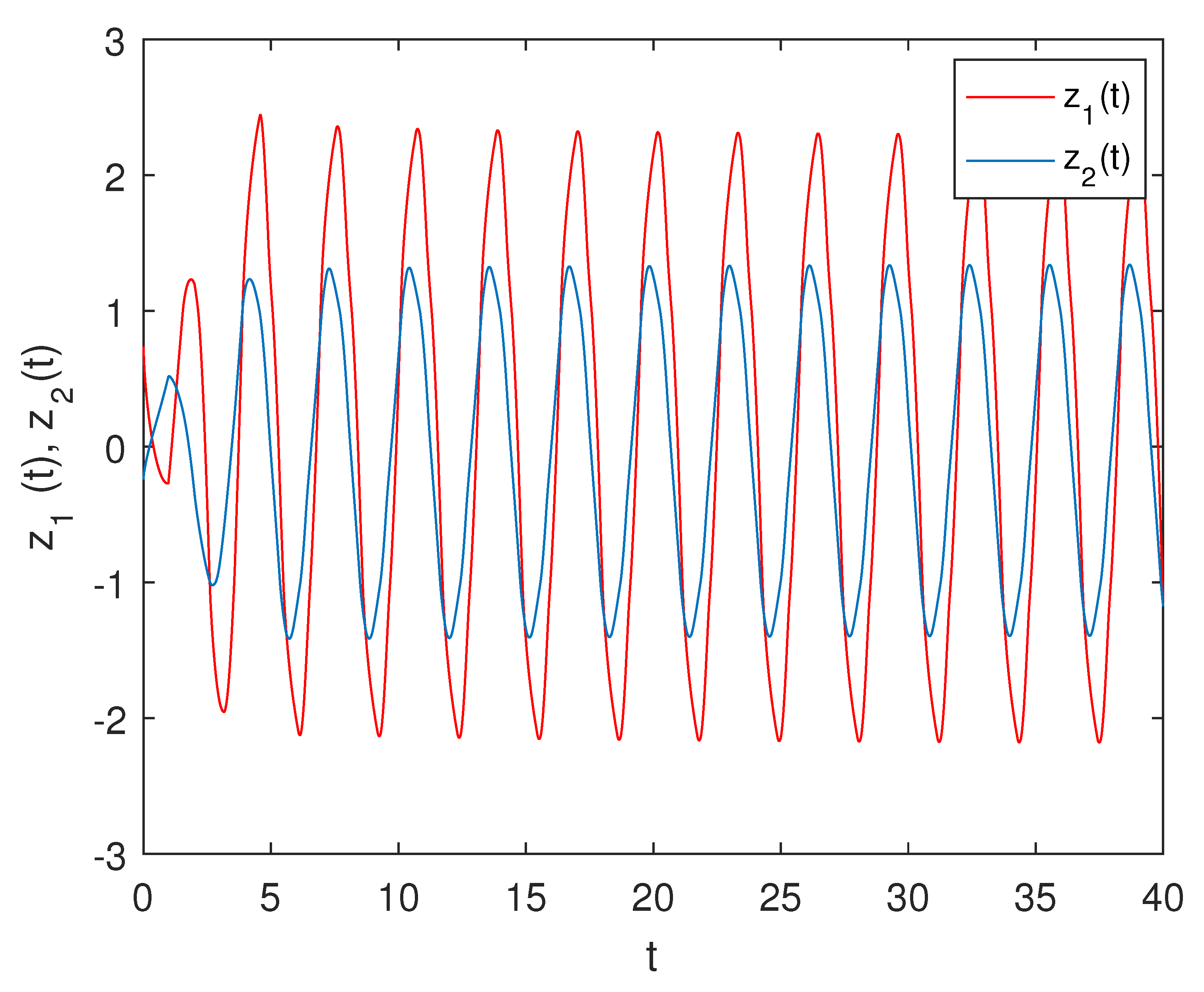
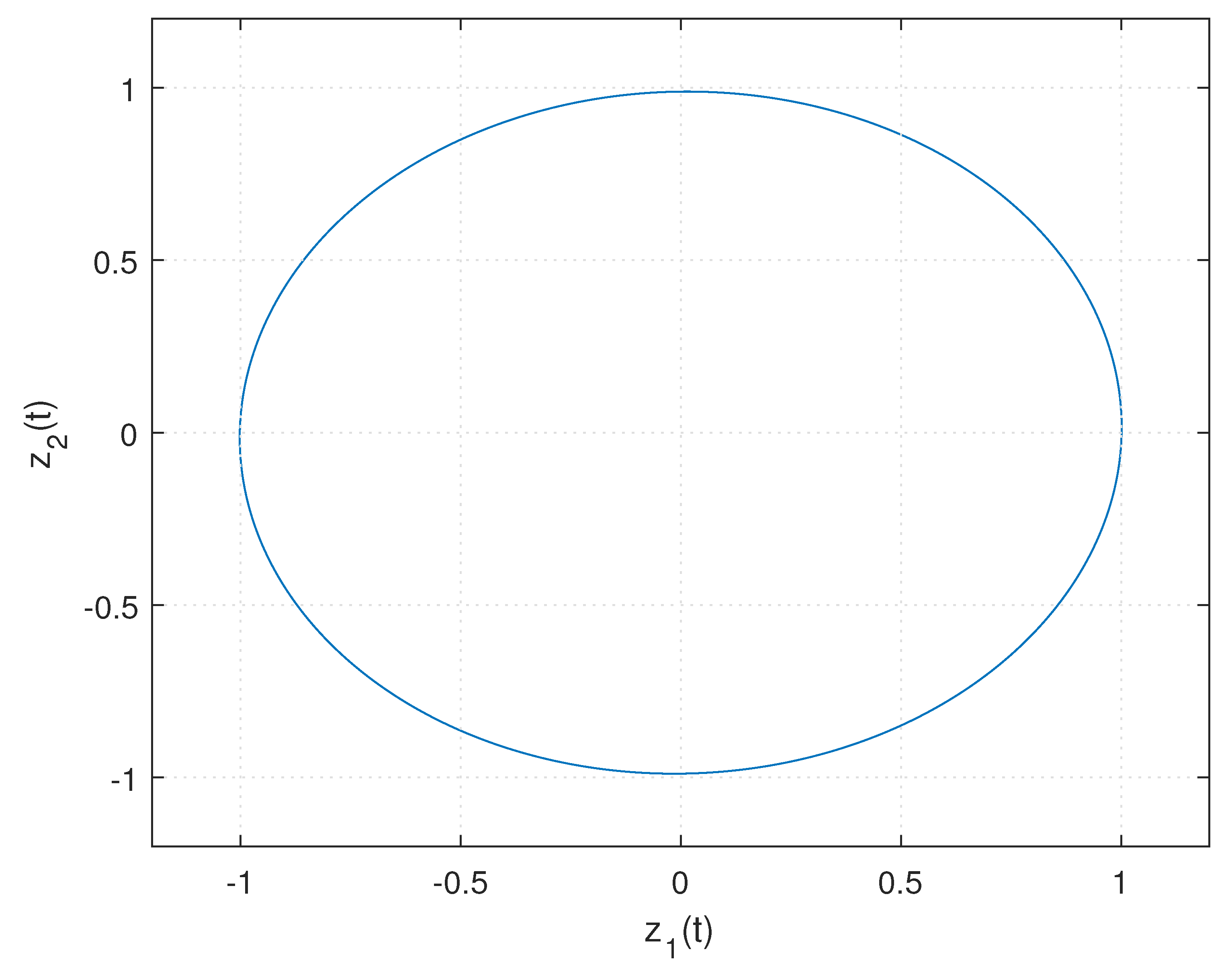
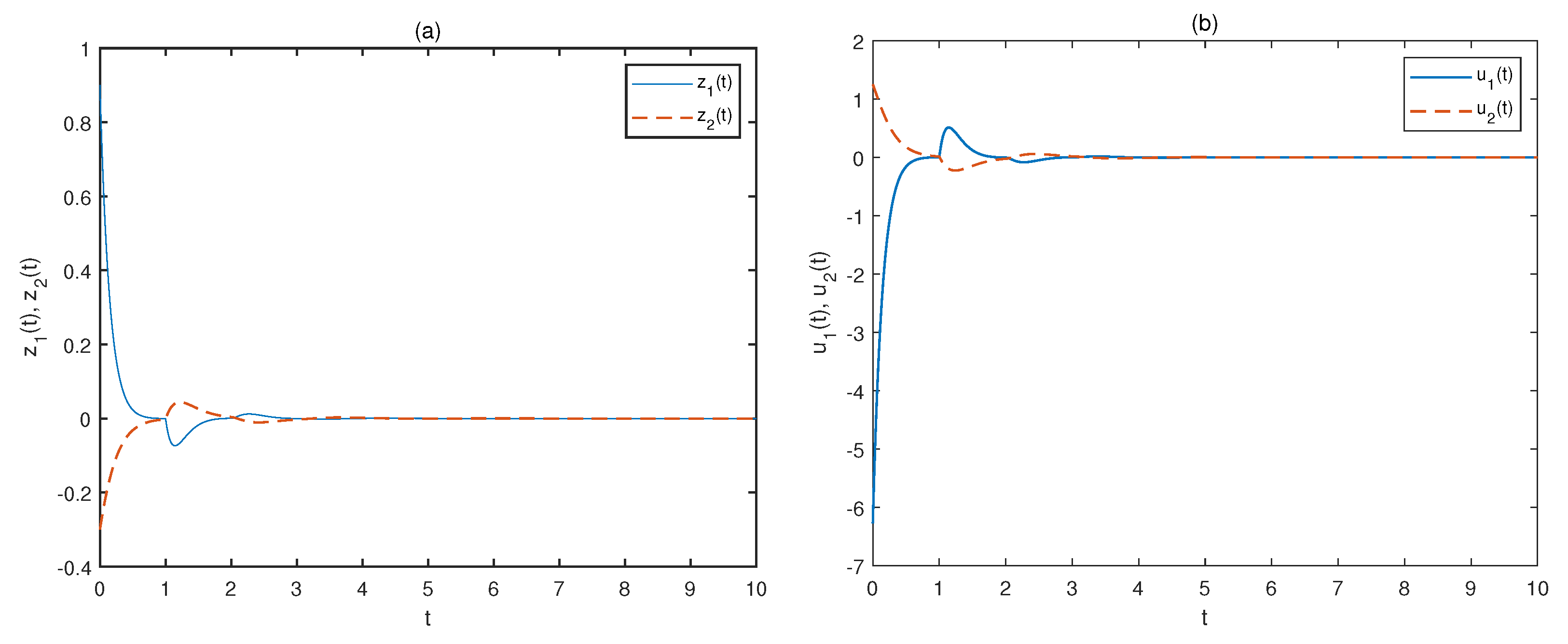
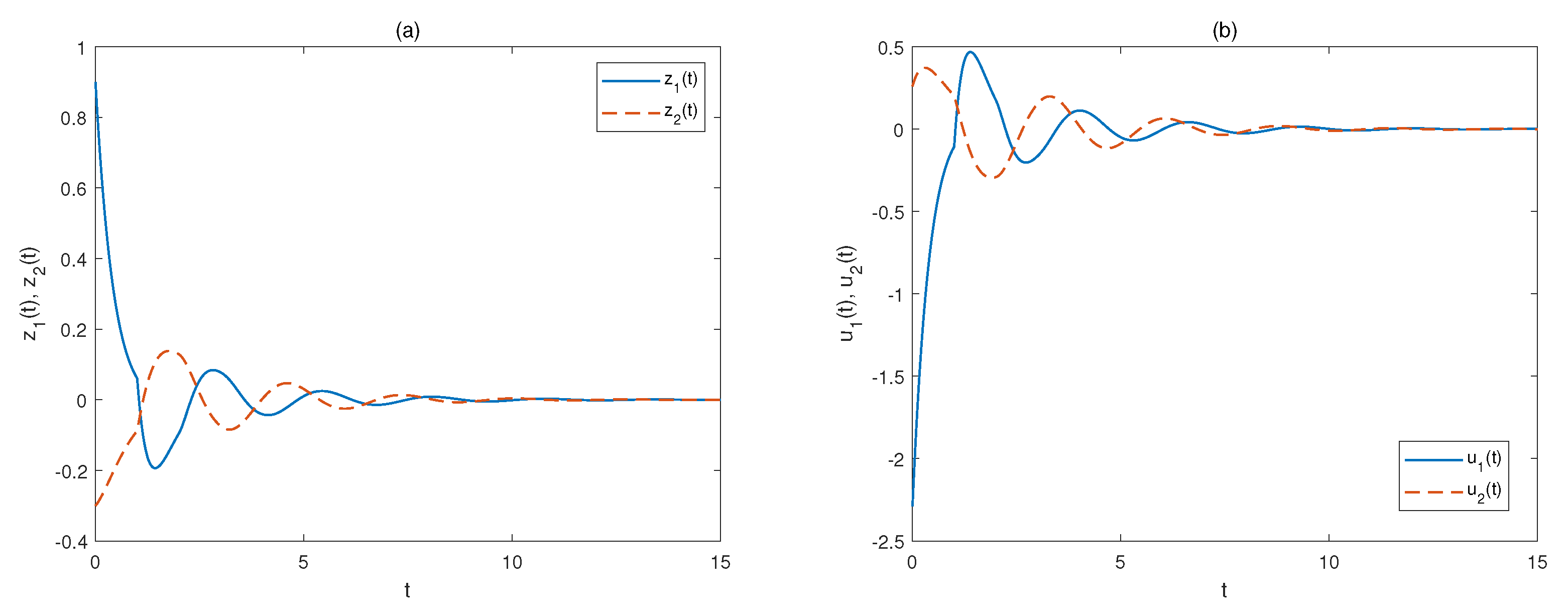
5. Numerical Examples

Example 1.

Consider a two-dimensional delayed FNNs (1) with $D=diag(1,1)$, $M=\left[\begin{array}{cc}1.7& 1.5\\ 0.1& 1.7\end{array}\right]$, $W=\left[\begin{array}{cc}-1.5& 0.1\\ 0.1& -1.5\end{array}\right]$, $\alpha =0.5$, $f_j\left(z_j\right)=\frac{1}{2}\left(\right|z_j\left(t\right)+1|-|z_j\left(t\right)-1\left|\right)$, $g_j\left(z_j(t-\varrho )\right)=\frac{1}{2}\left(\right|z_j(t-\varrho )+1|-|z_j(t-\varrho )-1\left|\right)$, $j=1,2$, $\varrho =1$. By simple calculation, we have $F=G=diag(1,1)$. Then, the open-loop system state with the initial value $z\left(s\right)={(0.9,-0.3)}^T$, $s\in [-1,0]$, is shown in Figure 1. Take $\delta =2.0$, $ϵ=1.8$ such that $\delta -ϵ>0$; then, the simulation results based on optimization scheme A and scheme B are given as follows.

I. 

Optimization scheme A for Example 1

Select $u_{\left(i\right)}=7$, $i=1,2$, $K=\left[\begin{array}{cc}-7& -0.1001\\ -0.61& -6\end{array}\right]$, $Q=\left[\begin{array}{cc}-0.01& -0.101\\ -0.02& -0.09\end{array}\right]$. Then, based on the optimization scheme A, one has $\mu =1.0314$, $N=\left[\begin{array}{cc}5.9576& 0\\ 0& 9.8954\end{array}\right]$, $U_1=\left[\begin{array}{cc}2.2848& 0\\ 0& 3.2104\end{array}\right]$, $U_2=\left[\begin{array}{cc}0.9083& 0\\ 0& 0.9893\end{array}\right]$. The largest set of admissible initial values is solved as

$$\eta \left(P\right)=\{z\in {\mathbb{R}}^n:z^T\left[\begin{array}{cc}0.9977& -0.0149\\ -0.0149& 1.0229\end{array}\right]z\le 1\},$$

which is displayed in Figure 2. It is easy to see that the initial value $z\left(s\right)={(0.9,-0.3)}^T$, $s\in [-1,0]$, belongs to $\eta \left(P\right)$.

Based on the obtained parameters, the simulation results about the trajectories of the system state $z\left(t\right)$ and the controller $u\left(t\right)$ are displayed in Figure 3. We can find that the closed-loop system (2) can achieve the asymptotical stability with the designed saturating controller.

II. 

Optimization scheme B for Example 1

Take the set as $\eta \left(P\right)=\{z\in {\mathbb{R}}^n:z^T\left[\begin{array}{cc}1& 0\\ 0& 1\end{array}\right]z\le 1\}$ and select ${\xi }_i=1$, $i=1,2$, $Q=\left[\begin{array}{cc}-0.01& -0.101\\ -0.02& -0.09\end{array}\right]$. Then, based on the scheme B, one can obtain $u_{\left(1\right)}=\sqrt{8.0131}=2.8307$, $u_{\left(2\right)}=\sqrt{7.2459}=2.6918$, $N=\left[\begin{array}{cc}9.8998& 0\\ 0& 10.3512\end{array}\right]$, $U_1=\left[\begin{array}{cc}2.2752& 0\\ 0& 3.0646\end{array}\right]$, $U_2=\left[\begin{array}{cc}0.9961& 0\\ 0& 1.0235\end{array}\right]$, and the control gain matrix $K=\left[\begin{array}{cc}-2.7772& -0.6975\\ -0.6165& -2.7149\end{array}\right]$. From Figure 4a,b, we can find that the closed-loop delayed FNNs (2) can achieve the asymptotical stability with the obtained saturating controller.

Example 2.

Consider a three-dimensional delayed FNNs (1), $D=diag(1,1,1)$, $M=\left[\begin{array}{ccc}0& 8& 0\\ 1& 0& 1\\ 0& -11& 1\end{array}\right]$, $W=\left[\begin{array}{ccc}2& 0& 0\\ 0.2& -0.1& 0\\ 9& 0& 0.1\end{array}\right]$, $\alpha =0.99$, $f_j\left(z_j\right)=tanh\left(z_j\right)$, $g_j\left(z_j(t-\varrho )\right)=tanh\left(z_j(t-\varrho )\right)$, $j=1,2,3$, $\varrho =3$. By simple calculation, one has $F=G=diag(1,1,1)$. Figure 5 shows the evolution of the system (2) without controller when $z\left(s\right)={(-0.6,0.3,0.8)}^T$, $s\in [-3,0]$. Take $\delta =1.2$, $ϵ=0.8$ such that $\delta -ϵ>0$; then, the simulation results are displayed in the following.

I. 

Optimization scheme A for Example 2

Select $K=\left[\begin{array}{ccc}-18& -0.1001& 0.01\\ -0.61& -12& -0.02\\ -0.05& 0.1& -13\end{array}\right]$, $Q=\left[\begin{array}{ccc}-0.01& -0.101& -0.02\\ -0.02& -0.09& -0.01\\ -0.02& 0.02& -0.08\end{array}\right]$, $u_{\left(i\right)}=15.6205$, $i=1,2,3$. Then, it yields $\mu =1.6007$,

$$N=\left[\begin{array}{ccc}10.4435& 0& 0\\ 0& 17.1171& 0\\ 0& 0& 8.2110\end{array}\right],U_1=\left[\begin{array}{ccc}13.3681& 0& 0\\ 0& 17.2440& 0\\ 0& 0& 0.2258\end{array}\right],$$

$$U_2=\left[\begin{array}{ccc}3.4473& 0& 0\\ 0& 0.1885& 0\\ 0& 0& 0.1408\end{array}\right],$$

and the region of admissible initial values (see Figure 6) is solved as

$$\eta \left(P\right)=\{z\in {\mathbb{R}}^n:z^T\left[\begin{array}{ccc}1.3508& 0.0040& 0.1242\\ 0.0040& 1.3736& -0.0181\\ 0.1242& -0.0181& 0.6956\end{array}\right]z\le 1\}.$$

In view of the derived control parameters, Figure 7a,b display the simulation results regarding the trajectories of the system state $z\left(t\right)$ and the controller $u\left(t\right)$, respectively. From Figure 7a,b, it can be found that the closed-loop system (2) can achieve the asymptotical stability by using the designed saturating controller.

II. 

Optimization Scheme B for Example 2

Take the set as $\eta \left(P\right)=\{z\in {\mathbb{R}}^n:z^T\left[\begin{array}{ccc}1& 0& 0\\ 0& 1& 0\\ 0& 0& 1\end{array}\right]z\le 1\}$ and select ${\xi }_j=1$, $j=1,2,3$, $Q=\left[\begin{array}{ccc}-0.01& -0.101& -0.02\\ -0.02& -0.09& -0.01\\ -0.02& 0.02& -0.08\end{array}\right]$. Then, using optimization scheme B, one can obtain $u_{\left(1\right)}=\sqrt{38.6229}=6.2147$, $u_{\left(2\right)}=\sqrt{29.8080}=5.4597$, $u_{\left(3\right)}=\sqrt{77.7384}=8.8169$,

$$N=\left[\begin{array}{ccc}11.2186& 0& 0\\ 0& 9.9823& 0\\ 0& 0& 11.5601\end{array}\right],U_1=\left[\begin{array}{ccc}10.1982& 0& 0\\ 0& 17.7403& 0\\ 0& 0& 1.0263\end{array}\right],$$

$$U_2=\left[\begin{array}{ccc}3.2529& 0& 0\\ 0& 0.1516& 0\\ 0& 0& 0.1460\end{array}\right],$$

and the control gain matrix K is solved as

$$K=\left[\begin{array}{ccc}-5.7046& -2.5859& -0.1582\\ -2.5049& -4.4700& 2.0992\\ -0.1582& 2.1292& -8.6398\end{array}\right].$$

As displayed in Figure 8a,b, it is easy to see that the response of closed-loop delayed FNNs (1) asymptotically converge to origin with the obtained controller. From the above analysis, the local stabilization can be successfully achieved for delayed FNNs subject to actuator saturation.

6. Conclusions

In this paper, the local stabilization problem is investigated for a class of delayed FNNs with actuator saturation. To obtain feedback control gain matrix, the dead-zone nonlinear function is used to deal with the saturation term. To derive the relevant stability results, the fractional-order Lyapunov theory and estimation technique of Mittag–Leffler function are utilized to establish an LMIs-based stability condition. To minimize the actuator costs and enlarge the region of admissible initial values, the convex optimization techniques are applied to develop two convex optimization schemes. Simulation results display that the proposed control scheme can guarantee the local stabilization for delayed FNNs with actuator saturation. In the future, the semi-global stabilization issue will be discussed for FNNs with actuator saturation and incommensurate orders. Nevertheless, two core issues are required to be answered: (1) How do we establish a fractional-order Lyapunov function by employing the pseudo-state variables? (2) How do we derive the fractional order $\alpha$-dependent optimization schemes by using the Riccati equation? In future research, we will discuss these topics.

References

1. Podlubny, I. Fractional Differential Equations; Academic Press: Cambridge, MA, USA, 1998. [Google Scholar]
2. Chen, L.; Chen, Y.; Lopes, A.M.; Kong, H.; Wu, R. State of charge estimation of lithium-ion batteries based on fuzzy fractional-order unscented kalman filter. Fractal Fract. 2021, 5, 91. [Google Scholar] [CrossRef]
3. Kaslik, E.; Sivasundaram, S. Nonlinear dynamics and chaos in fractional-order neural networks. Neural Net. 2012, 32, 245–256. [Google Scholar] [CrossRef] [PubMed]
4. Si, X.; Wang, Z.; Song, Z.; Zhang, Z. Asymptotic stabilization of delayed linear fractional-order systems subject to state and control constraints. Fractal Fract. 2022, 6, 67. [Google Scholar] [CrossRef]
5. Abdelouahab, M.S.; Lozi, R.; Chua, L.O. Memfractance: A mathematical paradigm for circuit elements with memory. Int. J. Bifurc. Chaos 2014, 24, 1430023. [Google Scholar] [CrossRef]
6. Lundstrom, B.N.; Higgs, M.H.; Spain, W.J.; Fairhall, A.L. Fractional differentiation by neocortical pyramidal neurons. Nat. Neurosci. 2008, 11, 1335–1342. [Google Scholar] [CrossRef]
7. Westerlund, S.; Ekstam, L. Capacitor theory. IEEE Trans. Dielect. Electron. Insul. 1994, 1, 826–839. [Google Scholar] [CrossRef]
8. Yu, Y.; Zhang, Z. State estimation for complex-valued inertial neural networks with multiple time delays. Mathematics 2022, 10, 1725. [Google Scholar] [CrossRef]
9. Ma, Q.; Xu, S. Consensus switching of second-order multiagent systems with time delay. IEEE Trans. Cybern. 2022, 52, 3349–3353. [Google Scholar] [CrossRef]
10. Wang, Z.; Wang, X.; Li, Y.; Haung, X. Stability and hopf bifurcation of fractional-order complex-valued single neuron model with time delay. Int. J. Bifurc. Chaos 2018, 27, 1750209. [Google Scholar] [CrossRef]
11. Yang, S.; Hu, C.; Yu, J.; Jiang, H. Exponential stability of fractional-order impulsive control systems with applications in synchronization. IEEE Trans. Cybern. 2020, 50, 3157–3168. [Google Scholar] [CrossRef]
12. Rajchakit, G.; Chanthorn, P.; Niezabitowski, M.; Raja, R.; Baleanu, D.; Pratap, A. Impulsive effects on stability and passivity analysis of memristor-based fractional-order competitive neural networks. Neurocomputing 2020, 417, 290–301. [Google Scholar] [CrossRef]
13. Wan, P.; Sun, D.; Zhao, M.; Zhao, H. Monostability and multistability for almost-periodic solutions of fractional-order neural networks with unsaturating piecewise linear activation functions. IEEE Trans. Neural Netw. Learn. Syst. 2020, 31, 5138–5152. [Google Scholar] [CrossRef]
14. Phat, V.N.; Thanh, N.T. New criteria for finite-time stability of nonlinear fractional-order delay systems: A Gronwall inequality approach. Appl. Math. Lett. 2018, 83, 169–175. [Google Scholar] [CrossRef]
15. Ding, Z.; Zeng, Z.; Wang, L. Robust finite-time stabilization of fractional-order neural networks with discontinuous and continuous activation functions under uncertainty. IEEE Trans. Neural Netw. Learn. Syst. 2018, 29, 1477–1490. [Google Scholar] [CrossRef]
16. Rajchakit, G.; Chanthorn, P.; Kaewmesri, P.; Sriraman, R.; Lim, C.P. Global Mittag-Leffler stability and stabilization analysis of fractional-order quaternion-valued memristive neural networks. Mathematics 2020, 8, 42. [Google Scholar] [CrossRef]
17. Yang, Z.; Zhang, J. Global stabilization of fractional-order bidirectional associative memory neural networks with mixed time delays via adaptive feedback control. Int. J. Comput. Math. 2020, 97, 2074–2090. [Google Scholar] [CrossRef]
18. Bao, H.; Park, J.; Cao, J. Adaptive synchronization of fractional-order output-coupling neural networks via quantized output control. IEEE Trans. Neural Netw. Learn. Syst. 2020, 32, 3230–3239. [Google Scholar] [CrossRef]
19. Zhang, S.; Yu, Y.; Yu, J. LMI conditions for global stability of fractional-order neural networks. IEEE Trans. Neural Netw. Learn. Syst. 2017, 28, 2423–2433. [Google Scholar] [CrossRef]
20. Fan, Y.; Huang, X.; Wang, Z.; Li, Y. Global dissipativity and quasi-synchronization of asynchronous updating fractional-order memristor-based neural networks via interval matrix method. J. Frankl. Inst. 2018, 355, 5998–6025. [Google Scholar] [CrossRef]
21. Chen, L.; Yin, H.; Wu, R.; Yin, L.; Chen, Y. Robust dissipativity and dissipation of a class of fractional-order uncertain linear systems. IET Control Theory Appl. 2019, 13, 1454–1465. [Google Scholar] [CrossRef]
22. Zhang, F.; Zeng, Z. Asymptotic stability and synchronization of fractional-order neural networks with unbounded time-varying delays. IEEE Trans. Syst. Man Cybern. Syst. 2021, 51, 5547–5556. [Google Scholar] [CrossRef]
23. Jia, J.; Wang, F.; Zeng, Z. Global stabilization of fractional-order memristor-based neural networks with incommensurate orders and multiple time-varying delays: A positive-system-based approach. Nonlinear Dyn. 2021, 104, 2303–2329. [Google Scholar] [CrossRef]
24. Gomes da Silva, M.; Tarbouriech, S. Anti-windup design with guaranteed region of stability: An LMI-based approach. IEEE Trans. Autom. Control 2005, 50, 1698–1711. [Google Scholar]
25. Seuret, A.; da Silva, M.G. Taking into account period variations and actuator saturation in sampled-data systems. Syst. Control Lett. 2012, 61, 1286–1293. [Google Scholar] [CrossRef]
26. Fan, Y.; Huang, X.; Wang, Z.; Xia, J.; Shen, H. Discontinuous event-triggered control for local stabilization of memristive neural networks with actuator saturation: Discrete-time and continuous-time Lyapunov methods. IEEE Trans. Neural Netw. Learn. Syst. 2021, 1–13. [Google Scholar] [CrossRef]
27. Chen, Y.; Wang, Z.; Shen, B.; Dong, H. Exponential synchronization for delayed dynamical networks via intermittent control: Dealing with actuator saturations. IEEE Trans. Neural Netw. Learn. Syst. 2019, 30, 1000–1012. [Google Scholar] [CrossRef]
28. Sun, W.; Wu, Y.; Lv, X. Adaptive neural network control for full-state constrained robotic manipulator with actuator saturation and time-varying delays. IEEE Trans. Neural Netw. Learn. Syst. 2022, 33, 3331–3342. [Google Scholar] [CrossRef]
29. Wei, Z.; Li, Q.; Che, J. Initial value problems for fractional differential equations involving riemann-liouville sequential fractional derivative. J. Math. Anal. Appl. 2010, 367, 260–272. [Google Scholar] [CrossRef]
30. Wang, D.; Xiao, A.; Liu, H. Dissipativity and stability analysis for fractional functional differential equations. Fract. Calc. Appl. Anal. 2015, 18, 1399–1422. [Google Scholar] [CrossRef]
31. Wu, Z.; Shi, P.; Su, H.; Chu, J. Local synchronization of chaotic neural networks with sampled-data and saturating actuators. IEEE Trans. Cybern. 2014, 44, 2635–2645. [Google Scholar]
32. Chen, G.; Sun, J.; Xia, J. Estimation of domain of attraction for aperiodic sampled-data switched delayed neural networks subject to actuator saturation. IEEE Trans. Neural Netw. Learn. Syst. 2020, 31, 1489–1503. [Google Scholar] [CrossRef]
33. Fan, Y.; Huang, X.; Wang, Z.; Li, Y. Quantised control for local Mittag-Leffler stabilization of fractional-order neural networks with input saturation: A refined sector condition. IET Contr. Theory Appl. 2021, 16, 366–376. [Google Scholar] [CrossRef]
34. Duarte-Mermoud, M.A.; Aguila-Camacho, N.; Gallegos, J.A.; Castro-Linares, R. Using general quadratic Lyapunov functions to prove Lyapunov uniform stability for fractional order systems. Commun. Nonlinear Sci. Numer. Simul. 2015, 22, 650–659. [Google Scholar] [CrossRef]
Figure 1. Response of the open-loop system state for Example 1.
Fractalfract 06 00451 g001
Figure 2. The set of admissible initial values for Example 1.
Fractalfract 06 00451 g002
Figure 3. Trajectories of (a): z ( t ) ; (b): u ( t ) of Example 1 based optimization scheme A.
Fractalfract 06 00451 g003
Figure 4. Trajectories of (a): z ( t ) ; (b): u ( t ) of Example 1 based on optimization scheme B.
Fractalfract 06 00451 g004
Figure 5. Trajectory of the open-loop system state for Example 2.
Fractalfract 06 00451 g005
Figure 6. The set of admissible initial values for Example 2.
Fractalfract 06 00451 g006
Figure 7. Trajectories of (a): z ( t ) ; (b): u ( t ) of Example 2 based on optimization scheme B.
Fractalfract 06 00451 g007
Figure 8. Trajectories of (a): z ( t ) ; (b): u ( t ) of Example 2 based on optimization scheme B.
Fractalfract 06 00451 g008